Poincaré Map for Discontinuous Fractional Differential Equations

Abstract

We work with a perturbed fractional differential equation with discontinuous right-hand sides where a discontinuity function crosses a discontinuity boundary transversally. The corresponding Poincaré map in a neighbourhood of a periodic orbit of an unperturbed equation is found. Then, bifurcations of periodic boundary solutions are analysed together with a concrete example.

1. Introduction

Many applications of fractional calculus and for discontinuous systems can be found in biophysics, quantum mechanics, group theory, robotics or economics. The main reason for the applications of fractional calculus is that fractional-order models have more degrees of freedom and are more flexible than the integer-order ones. On the other hand, discontinuous systems model phenomena with non-smooth forces or dry frictions. As basic sources are books such as [1,2,3,4,5,6], various analytical and numerical methods are applied as they are demonstrated in [7,8,9,10,11]. Moreover, the theory and applications of fractional systems are rapidly developing, supported by many recent papers and Special Issues such as [12,13,14,15,16], involving stability, asymptotic periodicity, synchronization, memory effect and several other important and interesting behaviours of fractional models.

We work with a perturbed fractional differential equation with globally Lipschitz right-hand sides and which change their forms, i.e., they are discontinuous and transversally cross a discontinuity boundary. We are looking for a solution of a perturbed system with a periodic boundary condition in a neighbourhood of a periodic orbit of an unperturbed system. That means a solution of an unperturbed equation is periodic. We consider Caputo fractional derivatives of an order less than one. Our approach is based on the well-known method of a Poincaré map constructed near an investigated periodic orbit widely applied in dynamical systems as either smooth or non-smooth [17,18]. Since our studied problem has a integral-differential structure due of using together integer and Caputo fractional derivatives, the extension of Poincaré method is not elementary, but rather technical. We also believe that it will have a good reason to continue in this study.

The paper is organised as follows. In Section 2, we introduce our problem and prove the existence of a global solution. In Section 3, we show the existence of a Poincaré map in a neighbourhood of a periodic orbit of an unperturbed equation, which allows a bifurcation analysis of periodic boundary solutions given in Section 4. Section 5 demonstrates our method on a concrete example, and it discusses a possible scenario of qualitative behaviour of our example problem. Section 6 summarises our achievements and proposes our future task.

2. Existence of Solutions

Let us consider the following equation:

$$x^{″}+{\mu }_1{}^C{D}_0^{q}x+g(x,x^{\prime })={\mu }_{2}h\left(x\right),$$

(1)

where $x\in \mathbb{R}$, $q\in (0,1)$, ${\mu }_1,{\mu }_2\in \mathbb{R}$ are small parameters, and function g is defined by

$$g(x,x^{\prime })=\left\{\begin{array}{cc}{g}_{+}\left(x\right)\hfill & \mathrm{for}{x}^{\prime }>0,\hfill \\ g_{-}\left(x\right)\hfill & \mathrm{for}{x}^{\prime }<0.\hfill \end{array}\right.$$

We suppose that functions $g_{\pm }$ and h are globally Lipschitz continuous functions on $\mathbb{R}$, and g transversally crosses the discontinuity boundary $x^{\prime }=0$, i.e., $g_{-}\left(x\right)g_{+}\left(x\right)>0$.

We say that $x\left(t\right)$ is a solution of the Equation (1) if it is continuous, piecewise $C^2$ and satisfies (1). The Equation (1) is equivalent to the following system:

$$\begin{array}{cc}\hfill x_1^{\prime }=& x_2,\hfill \\ \hfill x_2^{\prime }=& -{\mu }_1{}^C{D}_0^q{x}_1-g(x_1,x_2)+{\mu }_{2}h\left(x_1\right),\hfill \end{array}$$

(2)

where the second equation can be rewritten to the form

$$x_2^{\prime }=-{\mu }_1\frac{1}{\Gamma (1-q)}{\int }_0^t{(t-s)}^{-q}{x}_2\left(s\right)ds-g(x_1,x_2)+{\mu }_{2}h\left(x_1\right).$$

Initial conditions are as follows:

$$x_1\left(0\right)=u_0,x_2\left(0\right)=v_0.$$

We work with $v_0>0$.

Theorem 1. 

The solution $x=(x_1(u_0,v_0,{\mu }_1,{\mu }_2,t),x_2(u_0,v_0,{\mu }_1,{\mu }_2,t))$ of the system (2) with fixed $g(x_1,x_2)=g_{\pm }\left(x_1\right)$ exists on ${\mathbb{R}}_{+}=[0,\infty )$, and it is expressed as

$$\begin{array}{ccc}\hfill x_1& =& u_0+{\int }_0^t{x}_2\left(s\right)ds,\hfill \\ \hfill x_2& =& v_0-{\mu }_1\frac{1}{\Gamma (1-q)}{\int }_0^t{\int }_0^s{(s-z)}^{-q}{x}_2\left(z\right)dzds+{\int }_0^t(-g_{\pm }\left(x_1\left(s\right)\right)+{\mu }_{2}h\left(x_1\left(s\right)\right))ds.\hfill \end{array}$$

Proof. 

The existence of a solution is shown by using the Banach fixed point theorem on a Banach space $X=C{({\mathbb{R}}_{+},\mathbb{R})}^2$ with a norm

$${\parallel x\parallel }_a=\underset{[{\mathbb{R}}_{+}}{max}\parallel x\left(t\right)\parallel e^{-at},$$

where $a>0$ is specified below and $\parallel x\parallel =max\left\{\right|x_1|,|x_2\left|\right\}$ is a norm on ${\mathbb{R}}^2$. When $x\in C({\mathbb{R}}_{+},\mathbb{R})$, we use the same norm ${\parallel x\parallel }_a={max}_{[{\mathbb{R}}_{+}}\left|x\left(t\right)\right|e^{-at}$.

Consider $F=(F_1,F_2)$ as a functional $F(x_1,x_2;u_0,v_0,{\mu }_1,{\mu }_2)$, where

$$\begin{array}{cc}\hfill F_1(x_1,x_2;u_0,v_0,{\mu }_1,{\mu }_2)\left(t\right)& =u_0+{\int }_0^t{x}_2\left(s\right)ds,\hfill \\ \hfill F_2(x_1,x_2;u_0,v_0,{\mu }_1,{\mu }_2)\left(t\right)& =v_0-{\mu }_1\frac{1}{\Gamma (1-q)}{\int }_0^t{\int }_0^s{(s-z)}^{-q}{x}_2\left(z\right)dzds\hfill \\ & +{\int }_0^t(-g_{\pm }\left(x_1\left(s\right)\right)+{\mu }_{2}h\left(x_1\left(s\right)\right))ds.\hfill \end{array}$$

We show that there is a unique point x such that $x=F\left(x\right)$ for $x=(x_1,x_2)$. We now verify that F is contractive on X for a suitable $a>0$:

$$\begin{array}{c}|F_1(x_1,x_2;u_0,v_0,{\mu }_1,{\mu }_2)\left(t\right)-F_1(y_1,y_2;u_0,v_0,{\mu }_1,{\mu }_2)\left(t\right)|\\ =|u_0+{\int }_0^t{x}_2\left(s\right)ds-u_0-{\int }_0^t{y}_2\left(s\right)ds|\le {\int }_0^t|x_2\left(s\right)-y_2\left(s\right)|ds\\ \le {\int }_0^t{\parallel x-y\parallel }_a{e}^{as}ds\le {\parallel x-y\parallel }_a\frac{e^{at}}{a}\end{array}$$

(3)

for $x=(x_1,x_2)$ and $y=(y_1,y_2)$. Multiplying (3) by $e^{-at}$, we get:

$$\parallel F_1(x_1,x_2;u_0,v_0,{\mu }_1,{\mu }_2)-F_1(y_1,y_2;u_0,v_0,{\mu }_1,{\mu }_2){\parallel }_a\le \frac{1}{a}{\parallel x-y\parallel }_a.$$

The mapping $F_1$ is contractive if

$$a>1.$$

(4)

Next, we compute

$$\begin{array}{c}|F_2(x_1,x_2;u_0,v_0,{\mu }_1,{\mu }_2)\left(t\right)-F_2(y_1,y_2;u_0,v_0,{\mu }_1,{\mu }_2)\left(t\right)|\\ =|{\mu }_1\frac{1}{\Gamma (1-q)}{\int }_0^t{\int }_0^s{(s-z)}^{-q}(y_2\left(z\right)-x_2\left(z\right))dzds+{\int }_0^t(g_{\pm }\left(y_1\left(s\right)\right)-{\mu }_{2}h\left(y_1\left(s\right)\right)\\ -g_{\pm }\left(x_1\left(s\right)\right)+{\mu }_{2}h\left(x_1\left(s\right)\right)\left)ds\right|\le |{\mu }_1\frac{1}{\Gamma (1-q)}{\int }_0^t{\int }_0^s{(s-z)}^{-q}(y_2\left(z\right)-x_2\left(z\right))dzds|\\ +\left|{\int }_0^t(g_{\pm }\left(y_1\left(s\right)\right)-{\mu }_{2}h\left(y_1\left(s\right)\right)-g_{\pm }\left(x_1\left(s\right)\right)+{\mu }_{2}h\left(x_1\left(s\right)\right))ds\right|.\end{array}$$

(5)

First, the integral in (5) is evaluated as follows:

$$\begin{array}{c}\hfill \left|{\int }_0^t{\int }_0^s{(s-z)}^{-q}(y_2\left(z\right)-x_2\left(z\right))dzds\right|\le {\int }_0^t{\int }_0^s{(s-z)}^{-q}|y_2\left(z\right)-x_2\left(z\right)|dzds\\ \hfill \le {\int }_0^t{\int }_0^s{(s-z)}^{-q}{\parallel x-y\parallel }_a{e}^{az}dzds\end{array}$$

(6)

Now, we first use substitution $s-z=r$, then $ar=u$.

$${\int }_0^s{(s-z)}^{-q}{e}^{az}dz\le {\int }_0^{\infty }{r}^{-q}{e}^{a(s-r)}dr=e^{as}{\int }_0^{\infty }{r}^{-q}{e}^{-ar}dr=\frac{e^{as}}{a}{\int }_0^{\infty }(\frac{u}{a}{)}^{-q}{e}^{-u}du$$

$$=\frac{e^{as}}{a^{1-q}}{\int }_0^{\infty }{u}^{-q}{e}^{-u}du=\frac{e^{as}}{a^{1-q}}\Gamma (1-q)$$

Thus, integral (6) is bounded by

$${\int }_0^t{\int }_0^s{(s-z)}^{-q}{\parallel x-y\parallel }_a{e}^{az}dzds\le \frac{{\parallel x-y\parallel }_a}{a^{1-q}}\Gamma (1-q)\frac{e^{at}}{a}.$$

(7)

Now we use Lipschitz continuity of functions $g_{\pm }$ and h. Let $L_G$ be a Lipschitz constant of function $G_{\pm }\left(z\right)$, where $G_{\pm }\left(z\right)=g_{\pm }\left(z\right)-{\mu }_{2}h\left(z\right)$.

$$\begin{array}{c}\hfill \left|{\int }_0^t(G_{\pm }\left(y_1\left(s\right)\right)-G_{\pm }\left(x_1\left(s\right)\right))ds\right|\le {\int }_0^t|G_{\pm }\left(y_1\left(s\right)\right)-G_{\pm }\left(x_1\left(s\right)\right)|ds\\ \hfill \le {\int }_0^t{L}_G{\parallel x-y\parallel }_a{e}^{as}ds=L_G{\parallel x-y\parallel }_a\frac{e^{at}}{a}\end{array}$$

(8)

Using (5), (7), and (8) can be bounded by:

$$|F_2(x_1,x_2;u_0,v_0,{\mu }_1,{\mu }_2)\left(t\right)-F_2(y_1,y_2;u_0,v_0,{\mu }_1,{\mu }_2)\left(t\right)|\le (L_G+\frac{1}{a^{1-q}{\mu }_1}){\parallel x-y\parallel }_a\frac{e^{at}}{a},$$

which implies

$$\parallel F_2(x_1,x_2;u_0,v_0,{\mu }_1,{\mu }_2)-F_2(y_1,y_2;u_0,v_0,{\mu }_1,{\mu }_2){\parallel }_a\le (L_G+\frac{1}{a^{1-q}{\mu }_1})\frac{1}{a}{\parallel x-y\parallel }_a$$

This shows that $F_2$ is contractive if (4) holds along with

$$(L_G+\frac{1}{a^{1-q}{\mu }_1})\frac{1}{a}<1$$

a map $F=(F_1,F_2)$ has a unique fixed point. The proof is completed. □

3. Poincaré Map

The solution $x_2$ varies depending on $g_{\pm }$. If $x_2$ is non-negative, we work with $g_{+}$, otherwise we work with $g_{-}$. We will therefore look for times $t_1$ and $t_2$ where $x_2$ is equal to zero, where $g_{+}$ changes to $g_{-}$ and vice versa.

Let us discuss a case, where parameters ${\mu }_1$ and ${\mu }_2$ are equal to 0. System (2) will then be system of ordinary differential equations.

$$\begin{array}{cc}\hfill x_1^{\prime }=& x_2\hfill \\ \hfill x_2^{\prime }=& -g_{\pm }\left(x_1\right)\hfill \end{array}$$

(9)

For $T_0$-periodic solution of system (9) is

$$x\left(0\right)=x\left(T_0\right)$$

fulfilled. The fixed $T_0$-periodic solution of system (9) will be denoted by $x^0$. The initial condition can be written as

$$x^0\left(0\right)=(u,v).$$

The solution $x^0$ can be written in the terms of $x_1$ and $x_2$:

$$\begin{array}{cc}\hfill x_1^0\left(t\right)=& x_1(x_1\left(0\right),x_2\left(0\right),0,0,t)=x_1(u,v,0,0,t)\hfill \\ \hfill x_2^0\left(t\right)=& x_2(x_1\left(0\right),x_2\left(0\right),0,0,t)=x_2(u,v,0,0,t).\hfill \end{array}$$

(10)

The function $x_2^0$ is of class $C^1$ in all its variables.

Let us suppose the existence of $t_1$ and $t_2$ that $0<t_1<t_2<T_0$ and $x_2^0\left(t_1\right)=x_2^0\left(t_2\right)=0$. At these points, function $g_{\pm }$ changes its form from $g_{+}$ to $g_{-}$ and vice versa. We work with $v>0$, therefore $t\in [0,t_1]$ will be $g_{\pm }=g_{+}$, which means that $x_2$ will be of the following form:

$$x_2(u,v,0,0,t)=v-{\int }_0^t{g}_{+}\left(x_1\left(s\right)\right)ds.$$

It can be seen that $t_1$ can be identified as a function $t_1=t_1(u,v,0,0)$ that

$$x_2(u,v,0,0,t_1(u,v,0,0))=0.$$

In the case where parameters ${\mu }_1$ and ${\mu }_2$ are not equal to 0, we obtain for $t\in [0,t_1]$

$$\begin{array}{c}\hfill x_2(u,v,{\mu }_1,{\mu }_2,t)=v-\frac{{\mu }_1}{\Gamma (1-q)}{\int }_0^t{\int }_0^s{(s-z)}^{-q}{x}_2\left(z\right)dzds\\ \hfill +{\mu }_2{\int }_0^{t}h\left(x_1\left(s\right)\right)ds-{\int }_0^t{g}_{+}\left(x_1\left(s\right)\right)ds.\end{array}$$

(11)

Similarly, for $t_2$

$$x_2(u,v,0,0,t)=v-{\int }_0^{t_1}{g}_{+}\left(x_1\left(s\right)\right)ds-{\int }_{t_1}^t{g}_{-}\left(x_1\left(s\right)\right)ds,$$

where $t_2$ can be seen as a function $t_2=t_2(u,v,0,0)$, that

$$x_2(u,v,0,0,t_2(u,v,0,0))=0.$$

If ${\mu }_1$ and ${\mu }_2$ are not equal to 0, we obtain for $t\in [t_1,t_2]$

$$\begin{array}{c}\hfill x_2(u,v,{\mu }_1,{\mu }_2,t)=v-\frac{{\mu }_1}{\Gamma (1-q)}{\int }_0^{t_1}{\int }_0^s{(s-z)}^{-q}{x}_2\left(z\right)dzds\\ \hfill -\frac{{\mu }_1}{\Gamma (1-q)}{\int }_{t_1}^t{\int }_0^{t_1}{(s-z)}^{-q}{x}_2\left(z\right)dzds-\frac{{\mu }_1}{\Gamma (1-q)}{\int }_{t_1}^t{\int }_{t_1}^s{(s-z)}^{-q}{x}_2\left(z\right)dzds\\ \hfill +{\mu }_2{\int }_0^{t_1}h\left(x_1\left(s\right)\right)ds+{\mu }_2{\int }_{t_1}^{t}h\left(x_1\left(s\right)\right)ds-{\int }_0^{t_1}{g}_{+}\left(x_1\left(s\right)\right)ds-{\int }_{t_1}^t{g}_{-}\left(x_1\left(s\right)\right)ds.\end{array}$$

(12)

Similarly, for interval $[t_2,T]:$

$$\begin{array}{c}\hfill x_2(u,v,{\mu }_1,{\mu }_2,t)=v-\frac{{\mu }_1}{\Gamma (1-q)}{\int }_0^{t_2}{\int }_0^s{(s-z)}^{-q}{x}_2\left(z\right)dzds\\ \hfill -\frac{{\mu }_1}{\Gamma (1-q)}{\int }_{t_2}^t{\int }_0^{t_2}{(s-z)}^{-q}{x}_2\left(z\right)dzds-\frac{{\mu }_1}{\Gamma (1-q)}{\int }_{t_2}^t{\int }_{t_2}^s{(s-z)}^{-q}{x}_2\left(z\right)dzds\\ \hfill +{\mu }_2{\int }_0^{t_1}h\left(x_1\left(s\right)\right)ds+{\mu }_2{\int }_{t_1}^{t_2}h\left(x_1\left(s\right)\right)ds+{\mu }_2{\int }_{t_2}^{t}h\left(x_1\left(s\right)\right)ds\\ \hfill -{\int }_0^{t_1}{g}_{+}\left(x_1\left(s\right)\right)ds-{\int }_{t_1}^{t_2}{g}_{-}\left(x_1\left(s\right)\right)-{\int }_{t_2}^t{g}_{+}\left(x_1\left(s\right)\right)ds.\end{array}$$

(13)

First, let us look at the solution $x_2$ for ${\mu }_1$=${\mu }_2$=0. The solution can be written in the following way:

$$x_2\left(t\right)=\left\{\begin{array}{cc}{x}_{2,1}\left(t\right)\hfill & \mathrm{for}t\in [0,t_1],\hfill \\ x_{2,2}\left(t\right)\hfill & \mathrm{for}t\in [t_1,t_2],\hfill \\ x_{2,3}\left(t\right)\hfill & \mathrm{for}t\in [t_2,T].\hfill \end{array}\right.$$

(14)

It can be easily seen, that

$$\begin{array}{c}\hfill x_{2,1}\left(t_1\right)=x_{2,2}\left(t_1\right),\\ \hfill x_{2,2}\left(t_2\right)=x_{2,3}\left(t_2\right),\\ \hfill x_{2,3}\left(T\right)=x_{2,1}\left(0\right),\end{array}$$

where the last equation is result from T-periodicity.

The solution for ${\mu }_1$ and ${\mu }_2$ not equal to 0 can be written as $x_{2,1}$, $x_{2,2}$ and $x_{2,3}$ on corresponding intervals $[0,t_1]$, $[t_1,t_2]$ and $[t_2,T]$, where these solutions are from (11)–(13).

It can be seen, that derivatives of function $x_2$ with respect to t are non-zero for $t=t_1$ and $t=t_2.$

The solution $x_1\left(t\right)$ can be written similarly:

$$x_1\left(t\right)=\left\{\begin{array}{cc}{x}_{1,1}\left(t\right)\hfill & \mathrm{for}t\in [0,t_1],\hfill \\ x_{1,2}\left(t\right)\hfill & \mathrm{for}t\in [t_1,t_2],\hfill \\ x_{1,3}\left(t\right)\hfill & \mathrm{for}t\in [t_2,T].\hfill \end{array}\right.$$

(15)

$$\begin{array}{c}\hfill x_{1,1}\left(t_1\right)=x_{1,2}\left(t_1\right),\\ \hfill x_{1,2}\left(t_2\right)=x_{1,3}\left(t_2\right),\\ \hfill x_{1,3}\left(T\right)=x_{1,1}\left(0\right).\end{array}$$

Let us recall $x^0\left(t\right)$, a solution to an unperturbed Equation (1), i.e., for ${\mu }_1={\mu }_2=0$. $x^0\left(t\right)$ therefore indicates solutions (14) and (15). Now, we will look for a T-periodic boundary solution of system (2) near $x^0\left(t\right)$, which means that in system (2) we take ${\mu }_1$ and ${\mu }_2$ as small, close to 0. To reduce the number of variables, take ${\mu }_1$ and ${\mu }_2$ in the form $\epsilon {\widehat{\mu }}_1$ and $\epsilon {\widehat{\mu }}_2$, while $\epsilon$ will be taken small close to 0, and ${\widehat{\mu }}_1$ and ${\widehat{\mu }}_2$ can be any. For simplicity, we will rename the variables ${\widehat{\mu }}_1$ and ${\widehat{\mu }}_2$ to ${\mu }_1$ and ${\mu }_2$.

The system (2) can be written in the form

$$x^{\prime }=F_{\pm }\left(x\right)+\epsilon G\left(x\right),$$

(16)

that $x=\left(\begin{array}{c}{x}_1\\ x_2\end{array}\right)$, $F_{\pm }\left(x\right)=\left(\begin{array}{c}{x}_2\\ -g_{\pm }\left(x_1\right)\end{array}\right)$ and $\epsilon G\left(x\right)=\left(\begin{array}{c}0\\ \epsilon (-{\widehat{\mu }}_1{}^C{D}_0^q{x}_2+{\widehat{\mu }}_{2}h\left(x_1\right))\end{array}\right)$. Now we define Poincaré map. We choose $u_0=0$ and $v_0=\xi >0$.

$t_3$ is, similarly to $t_1$ and $t_2$, function of variables $\xi$ and $ϵ$, that defines as $x_1\left(t_3\right)=0$. $t_3$ determines the time, when solution meets its initial value, which can be seen in Figure 1 The Poincaré map is defined as

$$\tilde{P}(\xi ,\epsilon )=x_{+}(x_{-}\left(t_2\right),t_3,\epsilon ),$$

(17)

where $x_{+}(\xi ,\epsilon ,t)$ denotes the solution of (16) with $F_{+}\left(x\right)$ right-hand side and $x_{-}(\xi ,\epsilon ,t)$ the solution of (16) with $F_{-}\left(x\right)$ right-hand side. To find periodic boundary solution we solve the equation

$$\xi -\tilde{P}(\xi ,\epsilon )=0.$$

(18)

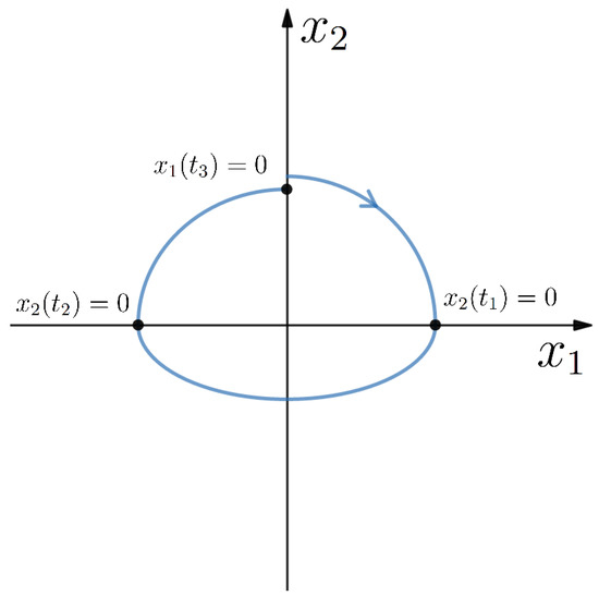
Figure 1. Graphical representation of the behaviour of the solution at times $t_1$, $t_2$ and $t_3$.

Differentiating the Equation (11) with respect to $\xi$ at the point $(\xi ,\epsilon )=(x_0,0)$ we obtain

$$x_2{(x_0,0,t)}_{\xi }=1-{\int }_0^t{g}_{+}^{\prime }\left(x_1\left(s\right)\right)x_{1\xi }\left(s\right)\left(s\right)ds.$$

(19)

In this case, we have $t\in [0,t_1]$, which gives us $g_{+}$ on the right-hand side. Differentiating the Equation (11) with respect to $\epsilon$ at the point $(\xi ,\epsilon )=(x_0,0)$, we have

$$\begin{array}{cc}\hfill x_2{(x_0,0,t)}_{\epsilon }=& -\frac{\widehat{{\mu }_1}}{\Gamma (1-q)}{\int }_0^t{\int }_0^s{(s-z)}^{-q}{x}_2\left(z\right)dzds\hfill \\ \hfill & +\widehat{{\mu }_2}{\int }_0^{t}h\left(x_1\left(s\right)\right)ds-{\int }_0^t{g}_{+}^{\prime }\left(x_1\right)x_{1\epsilon }\left(s\right)ds.\hfill \end{array}$$

(20)

Denote the first point, where $g_{+}$ changes to $g_{-}$ as ${\widehat{x}}_1$. $t_{1\xi }(x_0,0)$ can be obtained by differentiating (11) at $t=t_1(\xi ,\epsilon )$ with respect to $\xi$ as

$$t_{1\xi }(x_0,0)=\frac{1}{g_{+}\left({\widehat{x}}_1\right)}(1+{\int }_0^{t_1}{g}_{+}^{\prime }\left(x_1\left(s\right)\right)x_{1\xi }\left(s\right)ds).$$

(21)

Similarly, by differentiating with respect to $\epsilon$, we can express $t_{1\epsilon }$ as

$$\begin{array}{cc}\hfill t_{1\epsilon }(x_0,0)=& \frac{1}{g_{+}\left({\widehat{x}}_1\right)}(-\frac{\widehat{{\mu }_1}}{\Gamma (1-q)}{\int }_0^{t_1}{\int }_0^s{(s-z)}^{-q}{x}_2\left(z\right)dzds+\hfill \\ \hfill & +\widehat{{\mu }_2}{\int }_0^{t_1}h\left(x_1\left(s\right)\right)ds-{\int }_0^{t_1}{g}_{+}^{\prime }\left(x_1\right)x_{1\epsilon }\left(s\right)ds).\hfill \end{array}$$

(22)

Now, we take time $t\in [t_1,t_2]$, which gives us $g_{-}$ on the right-hand side. Differentiating (12) with respect to $\xi$ at the point $(\xi ,\epsilon )=({\widehat{x}}_1,0)$, we obtain

$$\begin{array}{cc}\hfill x_2{({\widehat{x}}_1,0,t)}_{\xi }=& 1-(t_{1\xi }{g}_{+}\left({\widehat{x}}_1\right)+{\int }_0^{t_1}{g}_{+}^{\prime }\left(x_1\left(s\right)\right)x_{1\xi }\left(s\right)ds-t_{1\xi }{g}_{-}\left({\widehat{x}}_1\right)\hfill \\ \hfill & +{\int }_{t_1}^t{g}_{-}^{\prime }\left(x_1\left(s\right)\right)x_{1\xi }\left(s\right)ds).\hfill \end{array}$$

(23)

Differentiating (12) with respect to and $\epsilon$ at the point $(\xi ,\epsilon )=({\widehat{x}}_1,0)$, we obtain

$$\begin{array}{cc}\hfill x_2{({\widehat{x}}_1,0,t)}_{\epsilon }=& -\frac{\widehat{{\mu }_1}}{\Gamma (1-q)}({\int }_0^{t_1}{\int }_0^s{(s-z)}^{-q}{x}_2\left(z\right)dzds\hfill \\ \hfill & +{\int }_{t_1}^t{\int }_0^{t_1}{(s-z)}^{-q}{x}_2\left(z\right)dzds+{\int }_{t_1}^t{\int }_{t_1}^s{(s-z)}^{-q}{x}_2\left(z\right)dzds)\hfill \\ \hfill & +\widehat{{\mu }_2}{\int }_0^{t}h\left(x_1\left(s\right)\right)ds-(g_{+}\left({\widehat{x}}_1\right)t_{1\epsilon }+{\int }_0^{t_1}{g}_{+}^{\prime }\left(x_1\right)x_{1\epsilon }\left(s\right)ds\hfill \\ \hfill & -g_{-}\left({\widehat{x}}_1\right)t_{1\epsilon }+{\int }_{t_1}^t{g}_{-}^{\prime }\left(x_1\right)x_{1\epsilon }\left(s\right)ds).\hfill \end{array}$$

(24)

For $t=t_2$ function $g_{-}$ changes to $g_{+}$. Denote by ${\widehat{x}}_2$ the point, when the change happens. Differentiating (12) at $t=t_2(\xi ,ϵ)$ with respect to $\xi$ and $\epsilon$, respectively, we have:

$$\begin{array}{cc}\hfill t_{2\xi }(x_0,0)=& \frac{1}{g_{-}\left({\widehat{x}}_2\right)}(1-{\int }_0^{t_1}{g}_{+}^{\prime }\left(x_1\left(s\right)\right)x_{1\xi }\left(s\right)ds-{\int }_{t_1}^{t_2}{g}_{-}^{\prime }\left(x_1\left(s\right)\right)x_{1\xi }\left(s\right)ds\hfill \\ \hfill & -\frac{1}{g_{+}\left({\widehat{x}}_1\right)}(1+{\int }_0^{t_1}{g}_{+}^{\prime }\left(x_1\left(s\right)\right)x_{1\xi }\left(s\right)ds)(g_{+}\left(x_1\right)-g_{-}\left(x_1\right))),\hfill \\ \hfill \end{array}$$

(25)

$$\begin{array}{cc}\hfill t_{2\epsilon }(x_0,0)=& \frac{1}{g_{-}\left({\widehat{x}}_2\right)}\left(\frac{\widehat{{\mu }_1}}{\Gamma (1-q)}\right({\int }_0^{t_1}{\int }_0^s{(s-z)}^{-q}{x}_2\left(z\right)dzds\hfill \\ \hfill & +{\int }_{t_1}^{t_2}{\int }_0^{t_1}{(s-z)}^{-q}{x}_2\left(z\right)dzds+{\int }_{t_1}^{t_2}{\int }_{t_1}^s{(s-z)}^{-q}{x}_2\left(z\right)dzds)\hfill \\ \hfill & -\widehat{{\mu }_2}{\int }_0^{t_2}h\left(x_1\left(s\right)\right)ds+{\int }_0^{t_1}{g}_{+}^{\prime }\left(x_1\right)x_{1\epsilon }\left(s\right)ds+{\int }_{t_1}^{t_2}{g}_{-}^{\prime }\left(x_1\right)x_{1\epsilon }\left(s\right)ds\hfill \\ \hfill & +(g_{+}\left(x_1\right)-g_{-}\left(x_1\right))\frac{1}{g_{+}\left({\widehat{x}}_1\right)}(-\frac{\widehat{{\mu }_1}}{\Gamma (1-q)}{\int }_0^{t_1}{\int }_0^s{(s-z)}^{-q}{x}_2\left(z\right)dzds\hfill \\ \hfill & +\widehat{{\mu }_2}{\int }_0^{t_1}h\left(x_1\left(s\right)\right)ds-{\int }_0^{t_1}{g}_{+}^{\prime }\left(x_1\right)x_{1\epsilon }\left(s\right)ds\left)\right).\hfill \end{array}$$

(26)

Now, take $t\in [t_2,t_3]$, and on the right-hand side of the equation is function $g_{+}$. Differentiating (13) with respect to $\xi$ and $\epsilon$ at the point $(\xi ,\epsilon )=({\widehat{x}}_2,0)$, respectively, we have:

$$\begin{array}{cc}\hfill x_2{({\widehat{x}}_2,0,t)}_{\xi }& =1-(t_{1\xi }{g}_{+}\left(x_1\right)+{\int }_0^{t_1}{g}_{+}^{\prime }\left(x_1\left(s\right)\right)x_{1\xi }\left(s\right)ds+t_{2\xi }{g}_{-}\left(x_1\right)-t_{1\xi }{g}_{-}\left(x_1\right)\hfill \\ \hfill & +{\int }_{t_1}^{t_2}{g}_{-}^{\prime }\left(x_1\left(s\right)\right)x_{1\xi }\left(s\right)ds-t_{2\xi }{g}_{+}\left(x_1\right)+{\int }_{t_2}^t{g}_{+}^{\prime }\left(x_1\left(s\right)\right)x_{1\xi }\left(s\right)ds),\hfill \end{array}$$

(27)

$$\begin{array}{cc}\hfill x_2{({\widehat{x}}_2,0,t)}_{\epsilon }=& -\left(\frac{\widehat{{\mu }_1}}{\Gamma (1-q)}\right({\int }_0^{t_2}{\int }_0^s{(s-z)}^{-q}{x}_2\left(z\right)dzds\hfill \\ \hfill & +{\int }_{t_2}^t{\int }_0^{t_2}{(s-z)}^{-q}{x}_2\left(z\right)dzds+{\int }_{t_2}^t{\int }_{t_2}^s{(s-z)}^{-q}{x}_2\left(z\right)dzds)\hfill \\ \hfill & +\left(\widehat{{\mu }_2}{\int }_0^{t}h\left(x_1\left(s\right)\right)ds\right)\hfill \\ \hfill & -(g_{+}\left(x_1\left(t_1\right)\right)t_{1\epsilon }+{\int }_0^{t_1}{g}_{+}^{\prime }\left(x_1\right)x_{1\epsilon }\left(s\right)ds+g_{-}\left(x_1\right)t_{2\epsilon }-g_{-}\left(x_1\right)t_{1\epsilon }\hfill \\ \hfill & +{\int }_{t_1}^{t_2}{g}_{-}^{\prime }\left(x_1\right)x_{1\epsilon }\left(s\right)ds-t_{2\epsilon }{g}_{+}\left(x_1\right)+{\int }_{t_2}^t{g}_{+}^{\prime }\left(x_1\right)x_{1\epsilon }\left(s\right)ds).\hfill \end{array}$$

(28)

4. Bifurcation Analysis

Poincaré map fulfils:

$$P(x_0,\epsilon )=\left(\begin{array}{c}0\\ Q(\xi ,\epsilon )\end{array}\right),$$

(29)

where $x_0=\left(\begin{array}{c}0\\ \xi \end{array}\right)$. Denote by $\overline{\xi }$ the point, for which the periodic orbit $x^0$ exists for $\epsilon =0$. Then, we consider

$$\xi \in (\overline{\xi }-\delta ,\overline{\xi }+\delta ),\xi \mapsto Q(\xi ,\epsilon ),$$

for $\delta >0.$ In our particular case, the function Q equals $x_{2,3}\left(t_3\right)$, where $t_3$ is the point, where

$x_{1,1}\left(0\right)=x_{1,3}\left(t_3\right)=0.$

Let $\epsilon =0$. It is easy to see that $\overline{\xi }$ solves

$$Q(\xi ,0)-\xi =0,$$

hence

$$Q(\overline{\xi },0)-\overline{\xi }=0.$$

By differentiating the equation with respect to $\xi$ at the point $\xi =\overline{\xi }$, two options can occur:

$$Q_{\xi }(\overline{\xi },0)\ne 1$$

or

$$Q_{\xi }(\overline{\xi },0)=1.$$

In the first option, we obtain a isolated periodic boundary orbit, which means that the equation has a unique solution $\xi =\Psi \left(\epsilon \right)$ that fulfils $\overline{\xi }=\Psi \left(0\right).$

In the second option, the bifurcation may occur. Let us look at the special, degenerated, case of the second option:

$$Q(\xi ,0)\equiv \xi .$$

(30)

In this case, we obtain several solutions, the one-parameter system of periodic solutions of the unperturbed system. Assume that (30) is fulfilled. Using Hadamard’s Lemma express $Q(\xi ,\epsilon )$ in the form:

$$Q(\xi ,\epsilon )=Q(\xi ,0)+Q(\xi ,\epsilon )-Q(\xi ,0)=Q(\xi ,0)+\epsilon Q_1(\xi ,\epsilon )=\xi +\epsilon Q_1(\xi ,\epsilon )$$

The equation

$$\epsilon Q_1(\xi ,\epsilon )=0$$

is obtained. After multiplying the equation by $\frac{1}{\epsilon }$ and giving $\epsilon =0$, we have:

$$Q_1(\xi ,0)=0.$$

(31)

According to the roots of Equation (31), the existence of periodic boundary orbits can be discussed. If Equation (31) has a unique non-degenerated solution $\xi =\overline{\xi }$ for $\xi \in (\xi -\delta ,\xi +\delta )$, we obtain a local unique periodic boundary solution.

If the equation has no solution, a periodic boundary orbit does not exist. If the equation has several solutions, we obtain several periodic boundary orbits. In our particular case of Equation (1), $Q_1(\xi ,\epsilon )$ can be found by differentiating (13) with respect to $\epsilon$. We use the notation ${\mu }_1=\epsilon \widehat{{\mu }_1}$ and ${\mu }_2=\epsilon \widehat{{\mu }_2}$, as introduced earlier in this chapter. For $\epsilon =0$:

$$\begin{array}{cc}\hfill Q_1(\xi ,0)=& -\frac{{\widehat{\mu }}_1}{\Gamma (1-q)}({\int }_0^{t_2}{\int }_0^s{(s-z)}^{-q}{x}_2\left(z\right)dzds\hfill \\ \hfill & +{\int }_{t_2}^{t_3}{\int }_0^{t_2}{(s-z)}^{-q}{x}_2\left(z\right)dzds+{\int }_{t_2}^{t_3}{\int }_{t_2}^s{(s-z)}^{-q}{x}_2\left(z\right)dzds)\hfill \\ \hfill & +\left({\widehat{\mu }}_2{\int }_0^{t_3}h\left(x_1\left(s\right)\right)ds\right)\hfill \\ \hfill & -(g_{+}\left({\widehat{x}}_1\right)t_{1\epsilon }+{\int }_0^{t_1}{g}_{+}^{\prime }\left(x_1\left(s\right)\right)x_{1\epsilon }\left(s\right)ds+g_{-}\left({\widehat{x}}_2\right)t_{2\epsilon }-g_{-}\left({\widehat{x}}_1\right)t_{1\epsilon }\hfill \\ \hfill & +{\int }_{t_1}^{t_2}{g}_{-}^{\prime }\left(x_1\left(s\right)\right)x_{1\epsilon }\left(s\right)ds+t_{3\epsilon }{g}_{+}\left({\widehat{x}}_3\right)-t_{2\epsilon }{g}_{+}\left({\widehat{x}}_2\right)+{\int }_{t_2}^{t_3}{g}_{+}^{\prime }\left(x_1\left(s\right)\right)x_{1\epsilon }\left(s\right)ds).\hfill \end{array}$$

(32)

Since $x_1\left(t_3\right)=0$, $t_{3\epsilon }$ can be expressed by differentiating $x_1$ with respect to $\epsilon$.

$$t_{3\epsilon }=-\frac{1}{x_2\left(t_3\right)}{\int }_0^{t_3}{x}_{2\epsilon }\left(s\right)ds.$$

(33)

Using (22), (26) and (33) we can express $Q_1(\xi ,\epsilon )$ for $\epsilon =0$:

$$\begin{array}{cc}\hfill Q_1(\xi ,0)=& -\frac{{\widehat{\mu }}_1}{\Gamma (1-q)}({\int }_0^{t_2}{\int }_0^s{(s-z)}^{-q}{x}_2\left(z\right)dzds\hfill \\ \hfill & +{\int }_{t_2}^{t_3}{\int }_0^{t_2}{(s-z)}^{-q}{x}_2\left(z\right)dzds+{\int }_{t_2}^{t_3}{\int }_{t_2}^s{(s-z)}^{-q}{x}_2\left(z\right)dzds)\hfill \\ \hfill & +\left({\widehat{\mu }}_2{\int }_0^{t_3}h\left(x_1\left(s\right)\right)ds\right)\hfill \\ \hfill & -\left(\right(g_{+}\left({\widehat{x}}_1\right)-g_{-}\left({\widehat{x}}_1\right)\left)\frac{1}{g_{+}\left({\widehat{x}}_1\right)}\right(-\frac{\widehat{{\mu }_1}}{\Gamma (1-q)}{\int }_0^{t_1}{\int }_0^s{(s-z)}^{-q}{x}_2\left(z\right)dzds\hfill \\ \hfill & +\widehat{{\mu }_2}{\int }_0^{t_1}h\left(x_1\left(s\right)\right)ds-{\int }_0^{t_1}{g}_{+}^{\prime }\left(x_1\left(s\right)\right)x_{1\epsilon }\left(s\right)ds)\hfill \\ \hfill & +(g_{-}\left({\widehat{x}}_2\right)-g_{+}\left({\widehat{x}}_2\right))\frac{1}{g_{-}\left({\widehat{x}}_2\right)}\left(\frac{\widehat{{\mu }_1}}{\Gamma (1-q)}\right({\int }_0^{t_1}{\int }_0^s{(s-z)}^{-q}{x}_2\left(z\right)dzds\hfill \\ \hfill & +{\int }_{t_1}^{t_2}{\int }_0^{t_1}{(s-z)}^{-q}{x}_2\left(z\right)dzds+{\int }_{t_1}^{t_2}{\int }_{t_1}^s{(s-z)}^{-q}{x}_2\left(z\right)dzds)\hfill \\ \hfill & -\widehat{{\mu }_2}{\int }_0^{t_2}h\left(x_1\left(s\right)\right)ds+{\int }_0^{t_1}{g}_{+}^{\prime }\left(x_1\left(s\right)\right)x_{1\epsilon }\left(s\right)ds+{\int }_{t_1}^{t_2}{g}_{-}^{\prime }\left(x_1\left(s\right)\right)x_{1\epsilon }\left(s\right)ds\hfill \\ \hfill & +(g_{+}\left(x_1\right)-g_{-}\left(x_1\right))\frac{1}{g_{+}\left({\widehat{x}}_1\right)}(-\frac{\widehat{{\mu }_1}}{\Gamma (1-q)}{\int }_0^{t_1}{\int }_0^s{(s-z)}^{-q}{x}_2\left(z\right)dzds\hfill \\ \hfill & +\widehat{{\mu }_2}{\int }_0^{t_1}h\left(x_1\left(s\right)\right)ds-{\int }_0^{t_1}{g}_{+}^{\prime }\left(x_1\left(s\right)\right)x_{1\epsilon }\left(s\right)ds\left)\right)-g_{+}\left({\widehat{x}}_3\right)\frac{1}{x_2\left(t_3\right)}{\int }_0^{t_3}{x}_{2\epsilon }\left(s\right)ds\hfill \\ \hfill & +{\int }_0^{t_1}{g}_{+}^{\prime }\left(x_1\left(s\right)\right)x_{1\epsilon }\left(s\right)ds+{\int }_{t_1}^{t_2}{g}_{-}^{\prime }\left(x_1\left(s\right)\right)x_{1\epsilon }\left(s\right)ds+{\int }_{t_2}^{t_3}{g}_{+}^{\prime }\left(x_1\left(s\right)\right)x_{1\epsilon }\left(s\right)ds).\hfill \end{array}$$

(34)

5. Example of the Specific Equation

In further research, we will solve the equation, where the degenerated case (30) occurs. Using methods described in a previous chapter, we will solve specific equations in the form of (1). Let us solve an Equation (1) in unperturbed form.

$$x^{″}+g_{\pm }\left(x\right)=0.$$

(35)

Equation (35) is equivalent to the system

$$\begin{array}{cc}\hfill x_1^{\prime }=& x_2\hfill \\ \hfill x_2^{\prime }=& -g_{\pm }\left(x_1\right).\hfill \end{array}$$

(36)

Let the function $g_{\pm }$ be such that there exists a periodic solution.

$$g_{\pm }\left(x_1\right)=\left\{\begin{array}{c}{x}_1,x_2\ge 0\hfill \\ 4x_1,x_2<0\hfill \end{array}\right.$$

(37)

It is obvious that the periodic solution of system (36) exists.

Figure 2 shows that the solution of the system (36) is periodic. For $x_2$ positive $g_{\pm }=x_1$, therefore, the solutions above the $x_1$ axis are circles. The solutions under the $x_1$ axis are ellipses, and the reason is that $g_{\pm }=4x_1$. We can look for the times $t_1$ and $t_2$, in which the function $g_{\pm }$ changes from $g_{+}$ to $g_{-}$ and vice versa. The solution of the system (36) for $t\in [0,t_1]$ equals

$$\begin{array}{c}\hfill x_1\left(t\right)=c_{1}cos\left(t\right)+c_{2}sin\left(t\right),\\ \hfill x_2\left(t\right)=c_{2}cos\left(t\right)-c_{1}sin\left(t\right).\end{array}$$

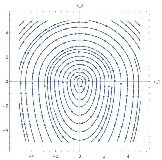
Figure 2. Local phase portrait of system (36).

$t_1$ is the first time in which the solution $x_2\left(t_1\right)=0.$ Because the time $t_1$ changes for different values of $c_1$ and $c_2$, we take the initial conditions as we used in the previous chapter, namely $x\left(0\right)=\left(\begin{array}{c}0\\ v_0\end{array}\right)$. In this case, the solution will be in the form of:

$$\begin{array}{cc}\hfill x_1\left(t\right)=& v_{0}sin\left(t\right),\hfill \\ \hfill x_2\left(t\right)=& v_{0}cos\left(t\right).\hfill \end{array}$$

(38)

Time $t_1$ will be the time when $x_2\left(t_1\right)=0.$ It is obvious that $t_1=\frac{\pi }{2}$. The system has on the interval $[\frac{\pi }{2},t_2]$ initial conditions $x_1\left(\frac{\pi }{2}\right)=v_0$ a $x_2\left(\frac{\pi }{2}\right)=0.$ Therefore, the solution is in the form

$$\begin{array}{cc}\hfill x_1\left(t\right)=& -v_{0}cos\left(2t\right),\hfill \\ \hfill x_2\left(t\right)=& 2v_{0}sin\left(2t\right).\hfill \end{array}$$

(39)

Hence, the time $t_2$, in which the function $g_{-}$ changes to $g_{+}$, is $t_2=\pi .$ Let us look for a T-periodic solution, which means, that the solutions $x_1\left(T\right)=x_1\left(0\right)$ and $x_2\left(T\right)=x_2\left(0\right)$. The solution for $t\in [\pi ,T]$ equals

$$\begin{array}{cc}\hfill x_1\left(t\right)=& v_{0}cos\left(t\right),\hfill \\ \hfill x_2\left(t\right)=& -v_{0}sin\left(t\right).\hfill \end{array}$$

(40)

Therefore, $T=\frac{3\pi }{2}$. Using the method described in the previous chapter, it is possible to find a Poincaré map for a perturbed equation

$$x^{″}+g_{\pm }\left(x\right)+\epsilon ({\mu }_1{}^C{D}_0^{q}x-{\mu }_{2}h\left(x\right))=0,$$

(41)

where $g_{\pm }\left(x\right)$ is determined by the relation (37) and $h\left(x\right)$ can be chosen as x, so $h\left(x\right)=x$. Solution x can be written as

$$\begin{array}{cc}\hfill x_1\left(t\right)& ={\int }_0^t{x}_2\left(s\right)ds\hfill \\ \hfill x_2\left(t\right)& =\xi -\epsilon {\mu }_1\frac{1}{\Gamma (1-q)}{\int }_0^t{\int }_0^s{(s-z)}^{-q}{x}_2\left(z\right)dzds+{\int }_0^t(-g_{\pm }\left(x_1\left(s\right)\right)+\epsilon {\mu }_2{x}_1\left(s\right)ds)\hfill \end{array}$$

In this case, we can express $Q_1$ as

$$\begin{array}{cc}\hfill Q_1(\xi ,0)=& -\frac{{\widehat{\mu }}_1}{\Gamma (1-q)}({\int }_0^{t_2}{\int }_0^s{(s-z)}^{-q}{x}_2\left(z\right)dzds\hfill \\ \hfill & +{\int }_{t_2}^{t_3}{\int }_0^{t_2}{(s-z)}^{-q}{x}_2\left(z\right)dzds+{\int }_{t_2}^{t_3}{\int }_{t_2}^s{(s-z)}^{-q}{x}_2\left(z\right)dzds)\hfill \\ \hfill & +\left({\widehat{\mu }}_2{\int }_0^{t_3}{x}_1\left(s\right)ds\right)\hfill \\ \hfill & -\left(\right({\widehat{x}}_1-4{\widehat{x}}_1\left)\frac{1}{{\widehat{x}}_1}\right(-\frac{\widehat{{\mu }_1}}{\Gamma (1-q)}{\int }_0^{t_1}{\int }_0^s{(s-z)}^{-q}{x}_2\left(z\right)dzds\hfill \\ \hfill & +\widehat{{\mu }_2}{\int }_0^{t_1}{x}_1\left(s\right)ds-{\int }_0^{t_1}4x_{1\epsilon }\left(s\right)ds)\hfill \\ \hfill & +(4{\widehat{x}}_2-{\widehat{x}}_2)\frac{1}{4{\widehat{x}}_2}\left(\frac{\widehat{{\mu }_1}}{\Gamma (1-q)}\right({\int }_0^{t_1}{\int }_0^s{(s-z)}^{-q}{x}_2\left(z\right)dzds\hfill \\ \hfill & +{\int }_{t_1}^{t_2}{\int }_0^{t_1}{(s-z)}^{-q}{x}_2\left(z\right)dzds+{\int }_{t_1}^{t_2}{\int }_{t_1}^s{(s-z)}^{-q}{x}_2\left(z\right)dzds)\hfill \\ \hfill & -\widehat{{\mu }_2}{\int }_0^{t_2}{x}_1\left(s\right)ds+{\int }_0^{t_1}{x}_{1\epsilon }\left(s\right)ds+{\int }_{t_1}^{t_2}4x_{1\epsilon }\left(s\right)ds\hfill \\ \hfill & +(\widehat{x_1}-4\widehat{x_1})\frac{1}{{\widehat{x}}_1}(-\frac{\widehat{{\mu }_1}}{\Gamma (1-q)}{\int }_0^{t_1}{\int }_0^s{(s-z)}^{-q}{x}_2\left(z\right)dzds\hfill \\ \hfill & +\widehat{{\mu }_2}{\int }_0^{t_1}{x}_1\left(s\right)ds-{\int }_0^{t_1}{x}_{1\epsilon }\left(s\right)ds\left)\right)-{\widehat{x}}_3\frac{1}{{\widehat{x}}_3}{\int }_0^{t_3}{x}_{2\epsilon }\left(s\right)ds\hfill \\ \hfill & +{\int }_0^{t_1}{x}_{1\epsilon }\left(s\right)ds+{\int }_{t_1}^{t_2}4x_{1\epsilon }\left(s\right)ds+{\int }_{t_2}^{t_3}{x}_{1\epsilon }\left(s\right)ds).\hfill \end{array}$$

(42)

where ${\widehat{x}}_1$, ${\widehat{x}}_2$ and ${\widehat{x}}_3$ are the first, second and third intersection points, respectively.

${\widehat{x}}_1=\left(\begin{array}{c}{x}_1\left(t_1\right)\\ x_2\left(t_1\right)\end{array}\right)=\left(\begin{array}{c}a\\ 0\end{array}\right)$, $a\in \mathbb{R}.$

${\widehat{x}}_2=\left(\begin{array}{c}{x}_1\left(t_2\right)\\ x_2\left(t_2\right)\end{array}\right)=\left(\begin{array}{c}b\\ 0\end{array}\right)$, $b\in \mathbb{R}.$

${\widehat{x}}_3=\left(\begin{array}{c}{x}_1\left(t_3\right)\\ x_2\left(t_3\right)\end{array}\right)=\left(\begin{array}{c}0\\ c\end{array}\right)$, $c\in \mathbb{R}.$

Times $t_1,t_2$ and $t_3$ satisfy following equations:

$$\begin{array}{cc}\hfill 0=x_2\left(t_1\right)=& \xi -\epsilon {\mu }_1\frac{1}{\Gamma (1-q)}{\int }_0^{t_1}{\int }_0^s{(s-z)}^{-q}{x}_2\left(z\right)dzds+(\epsilon {\mu }_2-1){\int }_0^{t_1}{x}_1\left(s\right)ds\hfill \\ \hfill 0=x_2\left(t_2\right)=& \xi -\frac{{\mu }_1}{\Gamma (1-q)}{\int }_0^{t_1}{\int }_0^s{(s-z)}^{-q}{x}_2\left(z\right)dzds\hfill \\ \hfill -& \frac{{\mu }_1}{\Gamma (1-q)}{\int }_{t_1}^{t_2}{\int }_0^{t_1}{(s-z)}^{-q}{x}_2\left(z\right)dzds-\frac{{\mu }_1}{\Gamma (1-q)}{\int }_{t_1}^{t_2}{\int }_{t_1}^s{(s-z)}^{-q}{x}_2\left(z\right)dzds\hfill \\ \hfill +& (\epsilon {\mu }_2-1){\int }_0^{t_1}{x}_1\left(s\right)ds+(\epsilon {\mu }_2-4){\int }_{t_1}^{t_2}{x}_1\left(s\right)ds\hfill \\ \hfill 0=x_1\left(t_3\right)=& {\int }_0^{t_3}{x}_2\left(s\right)ds\hfill \end{array}$$

To use (34) for our specific equation, we have to find functions $x_{1\epsilon }\left(t\right)$ and $x_{2\epsilon }$. Function $x_{2\epsilon }$ was defined (20), (24) and (28) on intervals [0,$t_1$],[$t_1$,$t_2$] and [$t_2,t_3$], respectively. Knowing that $x_1^{\prime }=x_2$ (2) (symbol ${}^{\prime }$ symbolizes the time derivative), we can formulate ODE system to find functions $x_{1\epsilon }\left(t\right)$ and $x_{2\epsilon }$ on each interval using functions (38), (39) and (40) as $x_1\left(t\right)$ and $x_2\left(t\right)$.

On interval [0,$t_1$] = [0,$\frac{\pi }{2}$], we have

$$\begin{array}{cc}\hfill x_{1\epsilon }^{\prime }=& x_{2\epsilon }\hfill \end{array}$$

(43)

$$\begin{array}{cc}\hfill x_{2\epsilon }^{\prime }=& -\frac{{\mu }_1}{\Gamma (1-q)}{\int }_0^t{(t-z)}^{-q}\xi coszdz+{\mu }_2\xi sint-x_{1\epsilon },\hfill \end{array}$$

(44)

with initial conditions $x_{1\epsilon }\left(0\right)=x_{2\epsilon }\left(0\right)=0.$ which, using a variation of parameters method, give the solution in the form:

$$\left(\begin{array}{c}{x}_{1\epsilon }\\ x_{2\epsilon }\end{array}\right)=e^{At}{\int }_0^t{e}^{-As}f\left(s\right)ds,$$

(45)

where $A=\left(\begin{array}{cc}0& 1\\ -1& 0\end{array}\right)$ and $f\left(t\right)=\left(\begin{array}{c}0\\ -\frac{{\mu }_1}{\Gamma (1-q)}{\int }_0^t{(t-z)}^{-q}\xi coszdz+{\mu }_2\xi sint\end{array}\right)$. Similarly, the ODE system on the second interval [$\frac{\pi }{2},\pi$]:

$$\begin{array}{cc}\hfill x_{1\epsilon }^{\prime }=& x_{2\epsilon }\hfill \end{array}$$

(46)

$$\begin{array}{cc}\hfill x_{2\epsilon }^{\prime }=& -\frac{{\mu }_1}{\Gamma (1-q)}({\int }_0^{\pi /2}{(t-z)}^{-q}\xi coszdz+{\int }_{\pi /2}^t{(t-z)}^{-q}2\xi sin2zdz)-{\mu }_2\xi cos2t+4x_{1\epsilon }.\hfill \end{array}$$

(47)

Its initial conditions can be calculated from Equation (45) at $t=\frac{\pi }{2}$. The solution on interval [$\frac{\pi }{2},\pi$] using a variation of parameters method is in the form:

$$\left(\begin{array}{c}{x}_{1\epsilon }\\ x_{2\epsilon }\end{array}\right)=e^{At}K+e^{At}{\int }_0^t{e}^{-As}f\left(s\right)ds,$$

(48)

where $A=\left(\begin{array}{cc}0& 1\\ 4& 0\end{array}\right)$, $K=e^{A\frac{\pi }{2}}\left(\begin{array}{c}{x}_{1\epsilon }\left(\frac{\pi }{2}\right)\\ x_{2\epsilon }\left(\frac{\pi }{2}\right)\end{array}\right)$

and $f\left(t\right)=\left(\begin{array}{c}0\\ -\frac{{\mu }_1}{\Gamma (1-q)}({\int }_0^{\pi /2}{(t-z)}^{-q}\xi coszdz+{\int }_{\pi /2}^t{(t-z)}^{-q}2\xi sin2zdz)-{\mu }_2\xi cos2t\end{array}\right)$.

On the last interval [$\pi ,\frac{3}{2}\pi$] is the ODE system in the form

$$\begin{array}{cc}\hfill x_{1\epsilon }^{\prime }=& x_{2\epsilon }\hfill \end{array}$$

(49)

$$\begin{array}{cc}\hfill x_{2\epsilon }^{\prime }=& -\frac{{\mu }_1}{\Gamma (1-q)}({\int }_0^{\pi /2}{(t-z)}^{-q}\xi coszdz+{\int }_{\pi /2}^{\pi }{(t-z)}^{-q}2\xi sin2zdz+\hfill \\ \hfill +& {\int }_{\pi /2}^t{(t-z)}^{-q}(-\xi )sinzdz)+{\mu }_2\xi cost-x_{1\epsilon },\hfill \end{array}$$

(50)

with initial conditions equal to (48) at time $t=\pi .$ The solution on interval [$\pi ,\frac{3}{2}\pi$] is in the form:

$$\left(\begin{array}{c}{x}_{1\epsilon }\\ x_{2\epsilon }\end{array}\right)=e^{At}K+e^{At}{\int }_0^t{e}^{-As}f\left(s\right)ds,$$

(51)

where $A=\left(\begin{array}{cc}0& 1\\ -1& 0\end{array}\right)$, $K=e^{A\pi }\left(\begin{array}{c}{x}_{1\epsilon }\left(\pi \right)\\ x_{2\epsilon }\left(\pi \right)\end{array}\right)$

and $f\left(t\right)=\left(\begin{array}{c}0\\ -& \frac{{\mu }_1}{\Gamma (1-q)}({\int }_0^{\pi /2}{(t-z)}^{-q}\xi coszdz+{\int }_{\pi /2}^{\pi }{(t-z)}^{-q}2\xi sin2zdz+\\ +& {\int }_{\pi /2}^t{(t-z)}^{-q}(-\xi )sinzdz)+{\mu }_2\xi cost\end{array}\right)$. We do not express analytical solutions (45), (48) and (51) in another form, because the given formulas lead to hypergeometric functions. For specific parameter choices, it is possible to find a numerical solution, but we do not go for details. We focus in this paper on the analytical theory of the Poincaré mapping method rather than its numerical investigation, which is interesting but postponed to another of our studies based on [19,20,21,22].

On the other hand, to understand the dynamics of (41), we first consider its limit case for $q=1$ (see [23]), so we have

$$\begin{array}{cc}\hfill x_1^{\prime }=& x_2\hfill \\ \hfill x_2^{\prime }=& -\frac{x_1(5-3sgn{x}_2)}{2}-\epsilon ({\mu }_1{x}_2-{\mu }_{2}h\left(x_1\right)),\hfill \end{array}$$

(52)

We see on Figure 3, Figure 4 and Figure 5 different dynamics depending on h. The perturbation $h\left(x_1\right)=x_1$ on Figure 3 keeps the symmetry along the origin. It seems that the origin is a global attractor. The perturbation $h\left(x_1\right)=x_1+10$ on Figure 4 breaks the symmetry along the origin. The perturbation $h\left(x_1\right)=x_1+x_1^3$ on Figure 5 keeps the symmetry along the origin, but it is nonlinear, and the dynamics are more interesting and complex.

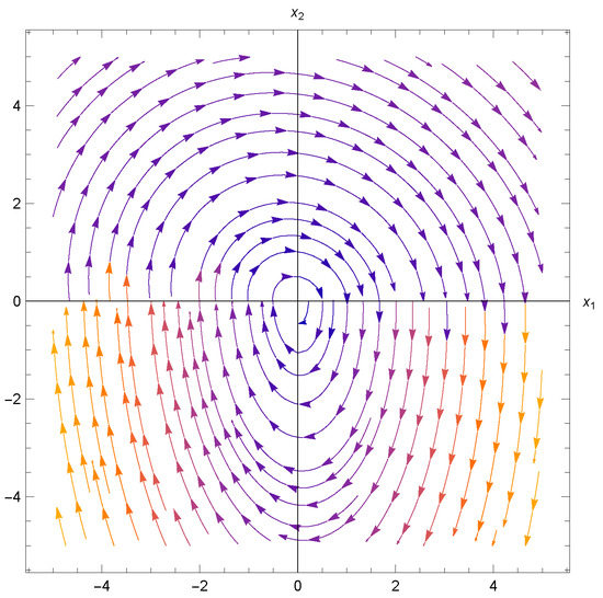
Figure 3. Local phase portrait of (52) for $\epsilon =0.1$, ${\mu }_1={\mu }_2=1$ and $h\left(x_1\right)=x_1$.

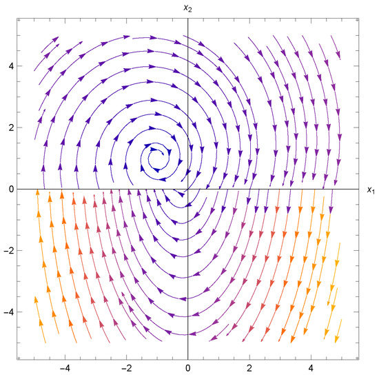
Figure 4. Local phase portrait of (52) for $\epsilon =0.1$, ${\mu }_1=1$, ${\mu }_2=-1$ and $h\left(x_1\right)=x_1+10$.

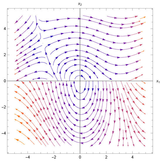
Figure 5. Local phase portrait of (52) for $\epsilon =0.1$, ${\mu }_1={\mu }_2=1$ and $h\left(x_1\right)=x_1+x_1^3$.

Next, we consider a limit case of (41) for $q=0$, so we have

$$\begin{array}{cc}\hfill x_1^{\prime }=& x_2\hfill \\ \hfill x_2^{\prime }=& -\frac{x_1(5-3sgn{x}_2)}{2}-\epsilon ({\mu }_1(x_1-x_1\left(0\right))-{\mu }_{2}h\left(x_1\right))\hfill \end{array}$$

(53)

(53) is no longer an ODE. For instance, if ${\mu }_1={\mu }_2=1$ and $h\left(x_1\right)=x_1$, we obtain

$$\begin{array}{cc}\hfill x_1^{\prime }=& x_2\hfill \\ \hfill x_2^{\prime }=& -\frac{x_1(5-3sgn{x}_2)}{2}+\epsilon x_2\left(0\right),\hfill \end{array}$$

(54)

The solutions of (54) seem to be repelled by Figure 6. Summarizing, the study of qualitative property of (41) is challenging by varying $q\in (0,1)$.

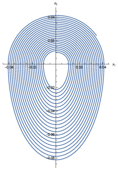
Figure 6. Solution of (54) for $\epsilon =0.1$ and $x_1\left(0\right)=0$, $x_2\left(0\right)=0.01$.

6. Conclusions

We work with a fractional differential equation with a discontinuous right-hand side, which is equivalent to the system (2). Suppose that functions $g_{\pm }$ are globally Lipschitz continuous, which change their form according to the sign of $x_2$ and transversally cross the discontinuity boundary.

We look for a periodic boundary solution of the system in a neighbourhood of the periodic orbit of an unperturbed system. That means the solution of the unperturbed equation is periodic.

We have shown the existence of the solution of the studied equation and found the corresponding Poincaré map in a neighbourhood of the periodic orbit of the unperturbed equation. We also present a bifurcation analysis of periodic boundary solutions.

We demonstrate how to apply our found formula to a concrete problem.

In the forthcoming work, we intend to generalize this theory to higher dimensions. Some of possible directions are outlined above.

References

- Di Bernardo, M. Piecewise-Smooth Dynamical Systems: Theory and Applications; Springer: London, UK, 2008. [Google Scholar]
- Kilbas, A.A.; Srivastava, H.M.; Trujillo, J.J. Theory and Applications of Fractional Differential Equations; Elsevier Science: Amsterdam, The Netherlands, 2006. [Google Scholar]
- Miller, K.S.; Ross, B. An Introduction to the Fractional Calculus and Differential Equations; John Wiley & Sons, Inc.: New York, NY, USA, 1993. [Google Scholar]
- Olejnik, P.; Awrejcewicz, J.; Fečkan, M. Modeling, Analysis and Control of Dynamical Systems: With Friction and Impacts; World Scientific Series on Nonlinear Science Series A: Volume 92; World Scientific Publishing Co. Pte. Ltd.: Singapore, 2018. [Google Scholar]
- Podlubny, I. Fractional Differential Equations. An Introduction to Fractional Derivatives, Fractional Differential Equations, Some Methods of Their Solution and Some of Their Applications; Academic Press: San Diego, CA, USA, 1999. [Google Scholar]
- Samko, S.; Kilbas, A.A.; Marichev, O. Fractional Integrals and Derivatives, Theory and Applications; Gordon and Breach Science Publishers: Amsterdam, The Netherlands, 1993. [Google Scholar]
- Kexue, L.; Jigen, P. Laplace transform and fractional differential equations. Appl. Math. Lett. 2011, 24, 2019–2023. [Google Scholar] [CrossRef]
- Diethelm, K. Monotonicity of functions and sign changes of their Caputo derivatives. Fract. Calc. Appl. Anal. 2016, 19, 561–566. [Google Scholar] [CrossRef]
- Evans, R.M.; Katugampola, U.N.; Edwards, D.A. Applications of fractional calculus in solving Abel-type integral equations: Surface–volume reaction problem. Comput. Math. Appl. 2017, 73, 1346–1362. [Google Scholar] [CrossRef]
- Podlubny, I. The Laplace Transform Method for Linear Differential Equations of the Fractional Order; Ústav Experimentálnej Fyziky SAV: Košice, Slovakia, 1994. [Google Scholar]
- Fečkan, M.; Pospíšil, M. On the bifurcation of periodic orbits in discontinuous systems. Commun. Math. Anal. 2010, 8, 87–108. [Google Scholar]
- Fečkan, M.; Sathiyaraj, T.; Wang, J.R. Synchronization of butterfly fractional order chaotic system. Mathematics 2020, 8, 446. [Google Scholar] [CrossRef]
- Fečkan, M.; Danca, M.-F. Stability, Periodicity, and Related Problems in Fractional-Order Systems. Mathematics 2022, 10, 2040. [Google Scholar] [CrossRef]
- Tarasov, V.E. General fractional vector calculus. Mathematics 2021, 9, 2816. [Google Scholar] [CrossRef]
- Tarasov, V.E. Exact solutions of Bernoulli and logistic fractional differential equations with power law coefficients. Mathematics 2020, 8, 2231. [Google Scholar] [CrossRef]
- Tarasov, V.E. Mathematical Economics: Application of Fractional Calculus. Mathematics 2020, 8, 660. [Google Scholar] [CrossRef]
- Fečkan, M.; Pospíšil, M. Poincaré-Andronov-Melnikov Analysis for Non-Smooth Systems; Elsevier: Amsterdam, The Netherlands, 2016. [Google Scholar]
- Guckenheimer, J.; Holmes, P. Nonlinear Oscillations, Dynamical Systems and Bifurcations of Vector Fields; Springer: New York, NY, USA, 1983. [Google Scholar]
- Fečkan, M.; Kelemen, S. Discretization of Poincaré map. Electron. J. Qual. Theory Differ. Equ. 2013, 60, 1–33. [Google Scholar] [CrossRef]
- Fečkan, M. Note on a Poincaré map. Math. Slovaca 1991, 41, 83–87. [Google Scholar]
- Cek, M.K.; Marek, M. Computational Methods in Bifurcation Theory and Dissipative Structures; Springer: New York, NY, USA, 1983. [Google Scholar]
- Henon, M. On the numerical computation of Poincaré maps. Phys. Nonlinear Phenom. 1982, 5, 412–414. [Google Scholar] [CrossRef]
- Fečkan, M.; Pospíšil, M.; Wang, J.R. Note on weakly fractional differential equations. Adv. Differ. Equ. 2019, 2019, 143. [Google Scholar] [CrossRef]
Publisher’s Note: MDPI stays neutral with regard to jurisdictional claims in published maps and institutional affiliations. |
© 2022 by the authors. Licensee MDPI, Basel, Switzerland. This article is an open access article distributed under the terms and conditions of the Creative Commons Attribution (CC BY) license (https://creativecommons.org/licenses/by/4.0/).