
Resiliency and Nonlinearity Profiles of Some Cryptographic Functions


Abstract
1. Introduction
2. Preliminaries
| Number of | ||
| 0 | ||
3. Computation of Disjoint Spectra Resilient Functions Having Good Nonlinearity
4. Lower Bounds for Fourth Order Nonlinearities of Two Classes of Monomial Functions Having Degree 5
- when
- when
- when
- when
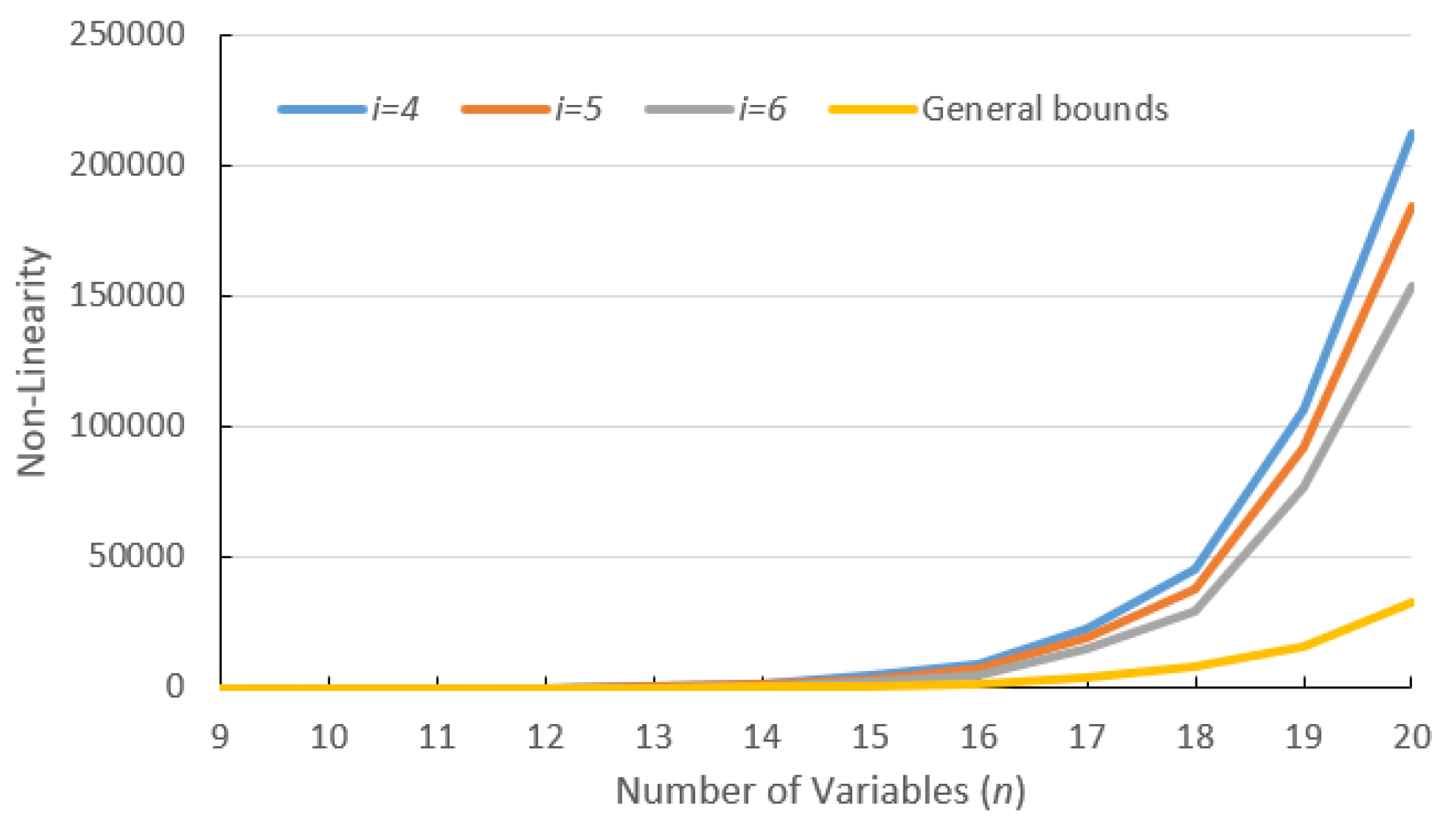
5. Comparison
6. Conclusions
Author Contributions
Funding
Institutional Review Board Statement
Informed Consent Statement
Data Availability Statement
Acknowledgments
Conflicts of Interest
References
- Rothaus, O. On “bent” functions. J. Comb. Theory Ser. 1976, 20, 300–305. [Google Scholar] [CrossRef]
- Golić, J.D. Fast Low Order Approximation of Cryptographic Functions. In Proceedings of the Advances in Cryptology—EUROCRYPT ’96; Maurer, U., Ed.; Springer: Berlin/Heidelberg, Germany, 1996; pp. 268–282. [Google Scholar]
- Iwata, T.; Kurosawa, K. Probabilistic Higher Order Differential Attack and Higher Order Bent Functions. In Proceedings of the Advances in Cryptology—ASIACRYPT ’99; Lam, K.Y., Okamoto, E., Xing, C., Eds.; Springer: Berlin/Heidelberg, Germany, 1999; pp. 62–74. [Google Scholar]
- Courtois, N.T. Higher Order Correlation Attacks, XL Algorithm and Cryptanalysis of Toyocrypt. In Proceedings of the Information Security and Cryptology—ICISC 2002; Lee, P.J., Lim, C.H., Eds.; Springer: Berlin/Heidelberg, Germany, 2003; pp. 182–199. [Google Scholar]
- Palit, S.; Roy, B.K.; De, A. A Fast Correlation Attack for LFSR-Based Stream Ciphers. In Proceedings of the Applied Cryptography and Network Security; Zhou, J., Yung, M., Han, Y., Eds.; Springer: Berlin/Heidelberg, Germany, 2003; pp. 331–342. [Google Scholar]
- Siegenthaler. Decrypting a Class of Stream Ciphers Using Ciphertext Only. IEEE Trans. Comput. 1985, C-34, 81–85. [Google Scholar] [CrossRef]
- Matsui, M. Linear Cryptanalysis Method for DES Cipher. In Proceedings of the Advances in Cryptology—EUROCRYPT ’93; Helleseth, T., Ed.; Springer: Berlin/Heidelberg, Germany, 1994; pp. 386–397. [Google Scholar]
- Sarkar, P.; Maitra, S. Nonlinearity Bounds and Constructions of Resilient Boolean Functions. In Proceedings of the Advances in Cryptology—CRYPTO 2000; Bellare, M., Ed.; Springer: Berlin/Heidelberg, Germany, 2000; pp. 515–532. [Google Scholar]
- Maitra, S.; Pasalic, E. Further constructions of resilient Boolean functions with very high nonlinearity. IEEE Trans. Inf. Theory 2002, 48, 1825–1834. [Google Scholar] [CrossRef]
- Zhang, W.; Xiao, G. Constructions of Almost Optimal Resilient Boolean Functions on Large Even Number of Variables. IEEE Trans. Inf. Theory 2009, 55, 5822–5831. [Google Scholar] [CrossRef]
- Carlet, C.; Charpin, P. Cubic Boolean functions with highest resiliency. IEEE Trans. Inf. Theory 2005, 51, 562–571. [Google Scholar] [CrossRef]
- Maitra, S.; Sarkar, P. Highly Nonlinear Resilient Functions Optimizing Siegenthaler’s Inequality. In Proceedings of the Advances in Cryptology—CRYPTO ’99; Wiener, M., Ed.; Springer: Berlin/Heidelberg, Germany, 1999; pp. 198–215. [Google Scholar]
- Pasalic, E.; Johansson, T. Further Results on the Relation Between Nonlinearity and Resiliency for Boolean Functions. In Proceedings of the Cryptography and Coding; Walker, M., Ed.; Springer: Berlin/Heidelberg, Germany, 1999; pp. 35–44. [Google Scholar]
- Huang, J.; Huang, Q.; Susilo, W. Leakage-resilient group signature: Definitions and constructions. Inf. Sci. 2020, 509, 119–132. [Google Scholar] [CrossRef]
- Gao, S.; Ma, W.; Zhao, Y.; Zhuo, Z. Walsh Spectrum of Cryptographically Concatenating Functions and Its Applications in Constructing Resilient Boolean Functions. J. Comput. Inf. Syst. 2011, 7, 1074–1081. [Google Scholar]
- Singh, D. Construction of Highly Nonlinear Plateaued Resilient Functions with Disjoint Spectra. In Proceedings of the CCIS; Balasubramaniam, P., Uthayakumar, R., Eds.; Springer: Berlin/Heidelberg, Germany, 2012; pp. 522–529. [Google Scholar]
- Carlet, C. Recursive Lower Bounds on the Nonlinearity Profile of Boolean Functions and Their Applications. IEEE Trans. Inf. Theory 2008, 54, 1262–1272. [Google Scholar] [CrossRef]
- Biham, E.; Shamir, A. Differential cryptanalysis of DES-like cryptosystems. J. Cryptol. 1991, 4, 3–72. [Google Scholar] [CrossRef]
- Fourquet, R.; Tavernier, C. An improved list decoding algorithm for the second order Reed–Muller codes and its applications. Des. Codes Cryptogr. 2008, 49, 323–340. [Google Scholar] [CrossRef]
- Sun, G.; Wu, C. The lower bounds on the second order nonlinearity of three classes of Boolean functions with high nonlinearity. Inf. Sci. 2009, 179, 267–278. [Google Scholar] [CrossRef]
- Gode, R.; Gangopadhyay, S. Third-order nonlinearities of a subclass of Kasami functions. Cryptogr. Commun. 2010, 2, 69–83. [Google Scholar] [CrossRef]
- Singh, D.; Paul, A. On 4th-order nonlinearity of a Subclass of Kasami Functions. In Proceedings of the 2nd International Conference on Science, Technology and Management; University of Delhi: New Delhi, India, 2015; pp. 1262–1269. [Google Scholar]
- Maitra, S.; Sarkar, P. Modifications of Patterson-Wiedemann functions for cryptographic applications. IEEE Trans. Inf. Theory 2002, 48, 278–284. [Google Scholar] [CrossRef]
- Siegenthaler, T. Correlation-immunity of nonlinear combining functions for cryptographic applications (Corresp.). IEEE Trans. Inf. Theory 1984, 30, 776–780. [Google Scholar] [CrossRef]
- Macwilliams, F.; Sloane, N. The Theory of Error Correcting Codes; North Holland Publishing: Amsterdam, The Netherlands, 2015; Volume 16. [Google Scholar]
- Bracken, C.; Byrne, E.; Markin, N.; McGuire, G. Determining the Nonlinearity of a New Family of APN Functions. In Proceedings of the Applied Algebra, Algebraic Algorithms and Error-Correcting Codes; Boztaş, S., Lu, H.F.F., Eds.; Springer: Berlin/Heidelberg, Germany, 2007; pp. 72–79. [Google Scholar]


| n | 7 | 11 | 15 | 19 | 23 |
|---|---|---|---|---|---|
| F and G in [15] | 64 | 15,872 | 258,048 | 4,161,536 | 66,846,720 |
| Functions in Theorem 3, [16] | 64 | 15,872 | 258,048 | 4,161,536 | 66,846,720 |
| in Theorem 3 | 96 | 16,128 | 260,096 | 4,177,920 | 66,977,792 |
| n | 9 | 10 | 11 | 12 | 13 | 14 | 15 | 16 | 17 | 18 | 19 | 20 | |
|---|---|---|---|---|---|---|---|---|---|---|---|---|---|
| Bounds of Theorem 4 | 22 | 43 | 163 | 326 | 937 | 1874 | 4797 | 9596 | 23,038 | 46,079 | 106,266 | 212,538 | |
| - | - | 85 | 170 | 651 | 1303 | 3750 | 7499 | 19,193 | 38,388 | 92,161 | 184,326 | ||
| - | - | - | - | 340 | 680 | 2606 | 5213 | 15,000 | 30,001 | 76,778 | 153,559 | ||
| General bounds in [17] | 16 | 32 | 64 | 128 | 256 | 512 | 1024 | 2048 | 4096 | 8192 | 16,384 | 32,768 | |
| n | 9 | 10 | 11 | 12 | 13 | 14 | 15 | 16 | 17 | 18 | 19 | 20 |
|---|---|---|---|---|---|---|---|---|---|---|---|---|
| Bounds of Theorem 5 | 22 | 43 | 163 | 326 | 937 | 1874 | 4797 | 9596 | 23,038 | 46,079 | 106,266 | 212,538 |
| Bounds for inverse function [17] | - | - | - | - | - | - | - | - | 2748 | 10,838 | 31,894 | 83,343 |
| Carlet’s general bounds [17] | 16 | 32 | 64 | 128 | 256 | 512 | 1024 | 2048 | 4096 | 8192 | 16,384 | 32,768 |
| Iwata-Kurosawa’s bounds [3] | 36 | 64 | 144 | 256 | 576 | 1024 | 2304 | 4096 | 9216 | 16,384 | 36,864 | 65,536 |
Publisher’s Note: MDPI stays neutral with regard to jurisdictional claims in published maps and institutional affiliations. |
© 2022 by the authors. Licensee MDPI, Basel, Switzerland. This article is an open access article distributed under the terms and conditions of the Creative Commons Attribution (CC BY) license (https://creativecommons.org/licenses/by/4.0/).
Share and Cite
Singh, D.; Paul, A.; Kumar, N.; Stoffová, V.; Verma, C. Resiliency and Nonlinearity Profiles of Some Cryptographic Functions. Mathematics 2022, 10, 4473. https://doi.org/10.3390/math10234473
Singh D, Paul A, Kumar N, Stoffová V, Verma C. Resiliency and Nonlinearity Profiles of Some Cryptographic Functions. Mathematics. 2022; 10(23):4473. https://doi.org/10.3390/math10234473
Chicago/Turabian StyleSingh, Deep, Amit Paul, Neerendra Kumar, Veronika Stoffová, and Chaman Verma. 2022. "Resiliency and Nonlinearity Profiles of Some Cryptographic Functions" Mathematics 10, no. 23: 4473. https://doi.org/10.3390/math10234473
APA StyleSingh, D., Paul, A., Kumar, N., Stoffová, V., & Verma, C. (2022). Resiliency and Nonlinearity Profiles of Some Cryptographic Functions. Mathematics, 10(23), 4473. https://doi.org/10.3390/math10234473