A Modified Inertial Parallel Viscosity-Type Algorithm for a Finite Family of Nonexpansive Mappings and Its Applications

Abstract

In this work, we aim to prove the strong convergence of the sequence generated by the modified inertial parallel viscosity-type algorithm for finding a common fixed point of a finite family of nonexpansive mappings under mild conditions in real Hilbert spaces. Moreover, we present the numerical experiments to solve linear systems and differential problems using Gauss–Seidel, weight Jacobi, and successive over relaxation methods. Furthermore, we provide our algorithm to show the efficiency and implementation of the LASSO problems in signal recovery. The novelty of our algorithm is that we show that the algorithm is efficient compared with the existing algorithms.

1. Introduction

Let $\mathcal{K}$ be a nonempty closed and convex subset of a real Hilbert space $\mathcal{H}$ and $T:\mathcal{K}\to \mathcal{K}$ be a mapping with the fixed point set $F\left(T\right)$, i.e., $F\left(T\right)=\{x\in \mathcal{K}:Tx=x\}$. A mapping T is said to be:

(1)

Contractive if there exists a constant $k\in (0,1)$ such that $\parallel Tx-Ty\parallel \le k\parallel x-y\parallel$ for all $x,y\in \mathcal{K}$;

(2)

Nonexpansive if $\parallel Tx-Ty\parallel \le \parallel x-y\parallel$ for all $x,y\in \mathcal{K}$.

Many problems in optimization can be solved by solving the transmission fixed point problem of a nonexpansive mapping, such as minimization problems, variational inequality, variational inclusion, etc. [1,2]. Thus, nonexpansive mapping has been studied extensively, including creating an algorithm to find its fixed point [3,4]. Constructing an algorithm to achieve strong convergence is a critical issue that many mathematicians focus on. One of them is the viscosity approximation method of selecting a particular fixed point of a given nonexpansive mapping as proposed by Moudafi [5] in 2000. Later, a class of viscosity-type methods was introduced by many authors; see [6,7]. One of the modified viscosity methods introduced by Aoyama and Kimura [8] is called the viscosity approximation method (VAM) for a countable family of nonexpansive mappings. The VAM was applied to a variational problem and zero point problem. When the contraction mappings are set by some fixed vectors, the VAM is reduced to a Halpern-type iteration method (HTI). To improve the convergence of the method, one of the most commonly used methods is the inertial method. In 1964, Polyak [9] introduced an algorithm that can speed up the gradient descent, and its modification was made immensely popular by Nesterov’s accelerated gradient algorithm, which was an algorithm proposed by Nesterov in 1983 [10]. This well-known method, which has improved the convergence rate, is known as the inertial iteration for the operator. Many researchers have given various acceleration techniques such as [11,12] to obtain a faster convergence method.

Many real-world problems can be modeled as common problems. Therefore, the study of the solving of these problem is important and has received the attention of many mathematicians. In 2015, Anh and Hieu [13] introduced a parallel monotone hybrid method (PMHM), and Khatibzadeh and Ranjbar [14] introduced Halpern-type iterations to approximate a finite family of quasi-nonexpansive mappingsin Banach space. Recently, there has been some research involving the parallel method for solving many problems. It is shown that the method can be applied in real-world problems such as image deblurring and related applications [15,16].

Inspired by previous works, in this work, we are interested in presenting a viscosity modification combined with the parallel monotone algorithm for a finite nonexpansive mapping. We provide a strong convergence theorem for the proposed algorithm with a parallel monotone algorithm. We provide numerical experiments of our algorithm for solving the linear system problem, differential problem, and signal recovery problem. The efficiency of the proposed algorithm is shown by comparing with existing algorithms.

2. Preliminaries

In this section, we give some definitions and lemmas that play an essential role in our analysis. The strong and weak convergence of $\left\{u_n\right\}$ to x will be denoted by $u_n\to u$ and $u_n\rightharpoonup u$, respectively. The projection of s on to A is defined by

$$P_A\left(s\right)=\underset{t\in A}{\mathrm{argmin}}\parallel s-t\parallel$$

where A is a nonempty, closed set.

Lemma 1

([17]). Let $\left\{s_n\right\}$ be a sequence of nonnegative real numbers such that there exists a subsequence $\left\{s_{n_i}\right\}$ of $\left\{s_n\right\}$ satisfying $\left\{s_{n_i}\right\}<\left\{s_{n_i+1}\right\}$ for all $i\in N$. Then, there exists a nondecreasing sequence $\left\{m_k\right\}$ of N such that ${\displaystyle \underset{k\to \infty }{lim}{m}_k=\infty }$ and the following properties are satisfied for all (sufficiently large) numbers $k\in N$:

$$s_{m_k}\le s_{m_k+1}\mathit{and}{s}_k\le s_{m_k+1}.$$

Lemma 2

([2]). Let $\left\{s_n\right\}$ be a sequence of nonnegative real numbers such that

$$s_{n+1}=(1-b_n)s_n+d_n$$

where $\left\{b_n\right\}\subset (0,1)$ with ${\displaystyle \sum _{n=0}^{\infty }{b}_n=\infty }$ and $\left\{d_n\right\}$ satisfies ${\displaystyle \underset{n\to \infty }{lim\; sup}{\displaystyle \frac{d_n}{b_n}}\le 0}$ or ${\displaystyle \sum _{n=0^{\infty }}\left|d_n\right|<\infty }$. Then, ${\displaystyle \underset{n\to \infty }{lim}{s}_n=0}$.

Lemma 3

([18]). Assume $\left\{s_n\right\}$ is a sequence of nonnegative real numbers such that

$$s_{n+1}\le (1-{\delta }_n)s_n+{\delta }_n{\tau }_n,n\ge 1$$

and

$$s_{n+1}\le s_n-{\eta }_n+{\rho }_n,n\ge 1.$$

where $\left\{{\delta }_n\right\}\subseteq (0,1)$, $\left\{{\eta }_n\right\}$ is a sequence of nonnegative real numbers, and $\left\{{\tau }_n\right\}$ and $\left\{{\rho }_n\right\}$ are real sequences such that:

• ${\displaystyle \sum _{n=1}^{\infty }{\delta }_n=\infty }$;
• ${\displaystyle \underset{n\to \infty }{lim}{\rho }_n=0}$;
• ${\displaystyle \underset{k\to \infty }{lim}{\eta }_{n_k}=0}$ implies ${\displaystyle \underset{k\to \infty }{lim\; sup}{\tau }_{n_k}\le 0}$ for any subsequence of real numbers $\left\{n_k\right\}$ of $\left\{n\right\}$.

Then, ${\displaystyle \underset{n\to \infty }{lim}{s}_n=0}$.

Proposition 1

([19]). Let H be a real Hilbert space. Let $m\in \mathbb{N}$ be fixed. Let ${\left\{x_i\right\}}_{i=1}^m\subset X$ and $t_i\ge 0$ for all $i=1,2,...,m$ with ${\displaystyle \sum _{i=1}^m{t}_i\le 1}$. Then, we have

$$\parallel \sum _{i=1}^m{t}_i{x}_i{\parallel }^2\le \frac{{\displaystyle \sum _{i=1}^m{t}_i{\parallel x_i\parallel }^2}}{{\displaystyle 2-\left(\sum _{i=1}^m{t}_i\right)}}.$$

(1)

3. Main Results

In this section, we introduce viscosity modification combined with the inertial parallel monotone algorithm for a finite family of nonexpansive mappings. Before proving the strong convergence theorem, we give the following Definition 1:

Definition 1.

Let C be a nonempty subset of a real Hilbert space H. Let $T_i:C\to C$ be nonexpansive mappings for all $i=1,2,...,N$. Then, ${\left\{T_i\right\}}_{i=1}^N$ is said to satisfy Condition (A)

if, for each bounded sequence $\left\{z_n\right\}\subset C$, there exists sequence $\left\{i_n\right\}$ such that $i_n\in \{1,2,...,N\}$ for all $n\ge 1$ with ${\displaystyle \underset{n\to \infty }{lim}\parallel z_n-T_{i_n}{z}_n\parallel =0}$ implying that ${\displaystyle \underset{n\to \infty }{lim}\parallel z_n-T_i{z}_n\parallel =0}$ for all $i=1,2,...,N$.

For the example of ${\left\{T_i\right\}}_{i=1}^N$, which satisfies Condition (A), we can set $T_i=J_{r_i}^{B_i}(I-r_i{A}_i)$, where $J_{r_i}^{B_i}={(I+r_i{B}_i)}^{-1}$, $A_i:H\to H$ is an ${\alpha }_i$-inverse strongly monotone operator, $B_i:H\to 2^H$ is a maximal monotone operator, and $r_i$ satisfies the assumptions in Theorem 3.1 of [1]. Assume that the following conditions hold:

C1.

${\displaystyle \underset{n\to \infty }{lim}\frac{{\theta }_n\parallel u_n-u_{n-1}\parallel }{{\alpha }_n}=0}$;

C2.

${\displaystyle \underset{n\to \infty }{lim}{\alpha }_n=0}$, ${\sum }_{n=1}^{\infty }{\alpha }_n=\infty$;

C3.

${\displaystyle \underset{n\to \infty }{lim\; inf}{\beta }_n{\gamma }_n>0}$, ${\displaystyle \underset{n\to \infty }{lim\; inf}{\beta }_n(1-{\alpha }_n-{\beta }_n-{\gamma }_n)>0}$.

Theorem 1.

Let $\left\{u_n\right\}$ be defined by Algorithm 1, and let ${\left\{T_i\right\}}_{i=1}^N$ satisfyCondition (A)such that ${\displaystyle F:=\bigcap _{i=1}^{N}F\left(T_i\right)\ne \varnothing }$. Then, the sequence $\left\{u_n\right\}$ converges strongly to $\overline{z}=P_{F}f\left(z\right).$

Algorithm 1: Let C be a nonempty closed convex subset of a real Hilbert space H, and let $f:H\to H$ be a contraction mapping. Let $T_i:C\to C$ be nonexpansive mappings for all $i=1,2,...,N$.

Suppose that $\left\{{\theta }_n\right\}\subset [0,\theta ]$ with $\theta \in [0,1)$ and $\left\{{\alpha }_n\right\}$, $\left\{{\beta }_n\right\}$, and $\left\{{\gamma }_n\right\}$ are sequences in $(0,1)$. For $n=1$, let $\left\{u_n\right\}$ be a sequence generated by $u_0,u_1\in H$, and define the following:   Step 1. Calculate the inertial step: $$v_n=u_n+{\theta }_n(u_n-u_{n-1}).$$ Step 2. Compute: $$s_{n,i}={\alpha }_{n}f\left(v_n\right)+{\beta }_n{v}_n+{\gamma }_n{T}_i{v}_n+(1-{\alpha }_n-{\beta }_n-{\gamma }_n)T_i\left(T_i{v}_n\right)$$ Step 3. Construct $u_{n+1}$ by $$u_{n+1}=\mathrm{argmax}\{\parallel s_{n,i}-v_n\parallel :i=1,2,...,N\}.$$ Step 4. Set $n=n+1$, and go to Step 1.

Proof. 

For each $n\in \mathbb{N},i\in \{1,2,...,N\}$, we set $\left\{z_{n,i}\right\}$ to be defined by $z_{1,i}\in H$ and

$$z_{n+1,i}={\alpha }_{n}f\left(z_{n,i}\right)+{\beta }_n{z}_{n,i}+{\gamma }_n{T}_i{z}_{n,i}+(1-{\alpha }_n-{\beta }_n-{\gamma }_n)T_i\left(T_i{z}_{n,i}\right).$$

Let $z\in F$. Then, for each $i\in \{1,2,...,N\}$, we have

$$\begin{array}{ccc}\hfill \parallel z_{n+1,i}-z\parallel & \le & {\alpha }_n\parallel f\left(z_{n,i}\right)-z\parallel +{\beta }_n\parallel z_{n,i}-z\parallel +{\gamma }_n\parallel T_i{z}_{n,i}-z\parallel \hfill \\ & & +(1-{\alpha }_n-{\beta }_n-{\gamma }_n)\parallel T_i\left(T_i{z}_{n,i}\right)-z\parallel \hfill \\ & \le & {\alpha }_n\parallel f\left(z_{n,i}\right)-f\left(z\right)\parallel +{\alpha }_n\parallel f\left(z\right)-z\parallel +(1-{\alpha }_n)\parallel z_{n,i}-z\parallel \hfill \\ & \le & (1-{\alpha }_n(1-k))\parallel z_{n,i}-z\parallel +{\alpha }_n\parallel f\left(z\right)-z\parallel \hfill \\ & =& (1-{\alpha }_n(1-k))\parallel z_{n,i}-z\parallel +{\alpha }_n(1-k)\frac{\parallel f\left(z\right)-z\parallel }{(1-k)}\hfill \\ & \le & max\left\{\parallel z_{n,i}-z\parallel ,\frac{\parallel f\left(z\right)-z\parallel }{(1-k)}\right\}\hfill \\ & ⋮& \hfill \\ & \le & max\left\{\parallel z_{1,i}-z\parallel ,\frac{\parallel f\left(z\right)-z\parallel }{(1-k)}\right\}.\hfill \end{array}$$

This shows that $\left\{z_{n,i}\right\}$ is bounded for all $i=1,2,...,N$. From the definition of $\left\{u_n\right\}$, there exist $i_n\in \{1,2,...,N\}$ such that

$$\begin{array}{c}\hfill u_{n+1}={\alpha }_{n}f\left(v_n\right)+{\beta }_n{v}_n+{\gamma }_n{T}_{i_n}{v}_n+(1-{\alpha }_n-{\beta }_n-{\gamma }_n)T_{i_n}\left(T_{i_n}{v}_n\right).\end{array}$$

(2)

Therefore, we obtain

$$\begin{array}{ccc}\hfill \parallel u_{n+1}-z_{n+1,i_n}\parallel & \le & {\alpha }_n\parallel f\left(v_n\right)-f\left(z_{n,i_n}\right)\parallel +{\beta }_n\parallel v_n-z_{n,i_n}\parallel +{\gamma }_n\parallel T_{i_n}{v}_n-T_{i_n}{z}_{n,i_n}\parallel \hfill \\ & & +(1-{\alpha }_n-{\beta }_n-{\gamma }_n)\parallel T_{i_n}\left(T_{i_n}{v}_n\right)-T_{i_n}\left(T_{i_n}{z}_{n,i_n}\right)\parallel \hfill \\ & \le & (1-{\alpha }_n(1-k))\parallel v_n-z_{n,i_n}\parallel \hfill \\ & \le & (1-{\alpha }_n(1-k))\parallel u_n+{\theta }_n(u_n-u_{n-1})-z_{n,i_n}\parallel \hfill \\ & \le & (1-{\alpha }_n(1-k))\parallel u_n-z_{n,i_n}\parallel +{\theta }_n\parallel u_n-u_{n-1}\parallel .\hfill \end{array}$$

By our assumptions and Lemma 2, we conclude that

$$\underset{n\to \infty }{lim}\parallel u_{n+1}-z_{n+1,i_n}\parallel =0.$$

(3)

By Proposition 1 and (2), we obtain

$$\begin{array}{c}\hfill \begin{array}{cc}\hfill \parallel z_{n+1,i_n}{-z\parallel }^2& =\parallel {\alpha }_n(f\left(z_{n,i_n}\right)-f\left(z\right))+{\alpha }_n(f\left(z\right)-z)+{\beta }_n(z_{n,i_n}-z)+{\gamma }_n(T_{i_n}{z}_{n,i_n}-z)\hfill \\ & +(1-{\alpha }_n-{\beta }_n-{\gamma }_n)(T_{i_n}{T}_{i_n}{z}_{n,i_n}-z){\parallel }^2\hfill \\ & \le \parallel {\alpha }_n(f\left(z_{n,i_n}\right)-f\left(z\right))+{\beta }_n(z_{n,i_n}-z)+{\gamma }_n(T_{i_n}{z}_{n,i_n}-z)\hfill \\ & +(1-{\alpha }_n-{\beta }_n-{\gamma }_n)(T_{i_n}{T}_{i_n}{z}_{n,i_n}-z){\parallel }^2+⟨{\alpha }_n(f\left(z\right)-z),z_{n+1,i_n}-z⟩\hfill \\ & \le {\alpha }_{n}k\parallel z_{n,i_n}{-z\parallel }^2+{\beta }_n\parallel z_{n,i_n}{-z\parallel }^2+(1-{\alpha }_n-{\beta }_n){\parallel T_{i_n}{z}_{n,i_n}-z_{n,i_n}\parallel }^2\hfill \\ & -{\beta }_n{\gamma }_n\parallel T_{i_n}{z}_{n,i_n}-z_{n,i_n}\parallel -{\beta }_n(1-{\alpha }_n-{\beta }_n-{\gamma }_n){\parallel T_{i_n}{T}_{i_n}{z}_{n,i_n}-z_{n,i_n}\parallel }^2\hfill \\ & +⟨{\alpha }_n(f\left(z\right)-z),z_{n+1,i_n}-z⟩\hfill \\ & \le (1-{\alpha }_n(1-k))\parallel z_{n,i_n}{-z\parallel }^2-{\beta }_n{\gamma }_n{\parallel T_{i_n}{z}_{n,i_n}-z_{n,i_n}\parallel }^2\hfill \\ & -{\beta }_n(1-{\alpha }_n-{\beta }_n-{\gamma }_n){\parallel T_{i_n}{T}_{i_n}{z}_{n,i_n}-z_{n,i_n}\parallel }^2\hfill \\ & +⟨{\alpha }_n(f\left(z\right)-z),z_{n+1,i_n}-z⟩.\hfill \end{array}\end{array}$$

(4)

Setting $s_n={\parallel z_{n,i_n}-z\parallel }^2$ implies that

$$\begin{array}{c}\hfill \begin{array}{cc}\hfill s_{n+1}& \le (1-{\alpha }_n(1-k))s_n-{\beta }_n{\gamma }_n{\parallel T_{i_n}{z}_{n,i_n}-z_{n,i_n}\parallel }^2\hfill \\ & -{\beta }_n(1-{\alpha }_n-{\beta }_n-{\gamma }_n){\parallel T_{i_n}{T}_{i_n}{z}_{n,i_n}-z_{n,i_n}\parallel }^2+⟨{\alpha }_n(f\left(z\right)-z),z_{n+1,i_n}-z⟩.\hfill \end{array}\end{array}$$

(5)

Assume that $u_n\to \overline{z}$, then we show that $\overline{z}\in F$. We will consider this for two possible cases on sequence $\left\{s_n\right\}$:

Case 1. Suppose that there exists $n_0\in \mathbb{N}$ such that $s_{n+1}\le s_n$ for all $n\ge n_0$. This implies that ${\displaystyle \underset{n\to \infty }{lim}{s}_n}$ exists. From (5), we have

$$\begin{array}{c}\hfill {\beta }_n{\gamma }_n{\parallel T_{i_n}{z}_{n,i_n}-z_{n,i_n}\parallel }^2\le (1-{\alpha }_n(1-k))s_n+⟨{\alpha }_n(f\left(z\right)-z),z_{n+1,i_n}-z⟩-s_{n+1}\end{array}$$

(6)

From Condition (A), (6), and $\left\{u_n\right\}$ bounded, we obtain

$$\begin{array}{c}\hfill \underset{n\to \infty }{lim}{\beta }_n{\gamma }_n{\parallel T_i{z}_{n,i_n}-z_{n,i_n}\parallel }^2=0\end{array}$$

(7)

From Condition C3 and (7), this implies that

$$\begin{array}{c}\hfill \underset{n\to \infty }{lim}\parallel T_{i_n}{z}_{n,i_n}-z_{n,i_n}\parallel =0\end{array}$$

As $u_n\to \overline{z}$ and ${\displaystyle \underset{n\to \infty }{lim}\parallel u_{n+1}-z_{n+1,i_n}\parallel =0}$ from (3), this implies that $z_{n,i_n}\to \overline{z}$. Since ${\left\{T_i\right\}}_{i=1}^N$ satisfies Condition (A), ${\displaystyle \underset{n\to \infty }{lim}\parallel T_i{z}_{n,i_n}-z_{n,i_n}\parallel =0}$ for all $i=1,2,...,N$. By the demiclosed property of nonexpansive mapping, we obtain ${\displaystyle \overline{z}\in F}$.

Case 2. Suppose that there exists a subsequence $\left\{s_{n_j}\right\}$ of $\left\{s_n\right\}$ such that $s_{n_j}<s_{n_j+1}$ for all $j\in \mathbb{N}$. In this case, it follows from Lemma 1 that there is a nondecreasing subsequence $\left\{m_k\right\}$ of N such that ${\displaystyle \underset{k\to \infty }{lim}{m}_k\to \infty }$, and the following inequalities hold for all $k\in N$:

$$s_{m_k}\le s_{m_k+1}\mathrm{and}{s}_k\le s_{m_k+1}.$$

Similar to Case 1, we obtain ${\displaystyle \underset{n\to \infty }{lim}\parallel T_{i_{m_k}}{z}_{m_k,i_{m_k}}-z_{m_k,i_{m_k}}\parallel =0}$. It is known that $u_n\to \overline{z}$, which implies $u_{m_k}\to \overline{z}$. Therefore, ${\displaystyle \overline{z}\in F}$. We next show that $\overline{z}=P_{F}f\left(z\right)$. From (4), we see that

$$\begin{array}{ccc}\hfill \parallel z_{n+1,i_n}{-z\parallel }^2& \le & (1-{\alpha }_n(1-k)){\parallel z_{n,i_n}-z\parallel }^2+⟨{\alpha }_n(f\left(z\right)-z),z_{n+1,i_n}-z⟩.\hfill \end{array}$$

Since $\left\{z_{n,i_n}\right\}$ is bounded, there exists a subsequence $\{\parallel z_{n_k,i_{n_k}}-z\parallel \}$ of $\{\parallel z_{n,i_n}-z\parallel \}$ such that

$${\displaystyle \underset{k\to \infty }{lim\; inf}(\parallel z_{n_k+1,i_{n_k}}-z\parallel -\parallel z_{n_k,i_{n_k}}-z\parallel )\ge 0\mathrm{and}\underset{k\to \infty }{lim\; sup}⟨f\left(z\right)-z,z_{n_k+1,i_{n_k}}-z⟩\le 0.}$$

For this purpose, one assumes that $\{\parallel z_{n_k,i_{n_k}}-z\parallel \}$ is a subsequence of $\{\parallel z_{n,i_n}-z\parallel \}$ such that ${\displaystyle \underset{k\in \infty }{lim\; inf}(\parallel z_{n_k+1,i_{n_k}}-z\parallel -\parallel z_{n_k,i_{n_k}}-z\parallel )\ge 0}$. This implies that

$$\begin{array}{ccc}& & \underset{k\to \infty }{lim\; inf}(\parallel z_{n_k+1,i_{n_k}}{-z\parallel }^2-\parallel z_{n_k,i_{n_k}}-z{\parallel }^2)\hfill \\ & =& \underset{k\to \infty }{lim\; inf}\left(\right(\parallel z_{n_k+1,i_{n_k}}-z\parallel -\parallel z_{n_k,i_{n_k}}-z\parallel \left)\right(\parallel z_{n_k+1,i_{n_k}}-z\parallel +\parallel z_{n_k,i_{n_k}}-z\parallel \left)\right)\hfill \\ & \ge & 0.\hfill \end{array}$$

From the definition of $z_n$, we obtain

$$\begin{array}{c}\hfill \begin{array}{cc}\hfill \parallel z_{n_k+1,i_{n_k}}-z_{n_k,i_{n_k}}\parallel & \le \parallel {\alpha }_{n_k}(f\left(z_{n_k,i_{n_k}}\right)-z_{n_k,i_{n_k}})+{\gamma }_{n_k}(T_{i_{n_k}}{z}_{n_k,i_{n_k}}-z_{n_k,i_{n_k}})\hfill \\ & +(1-{\alpha }_{n_k}-{\beta }_{n_k}-{\gamma }_{n_k})(T_{i_{n_k}}{T}_{i_{n_k}}{z}_{n_k,i_{n_k}}-z_{n_k,i_{n_k}})\parallel \hfill \\ & \le {\alpha }_{n_k}\parallel f\left(z_{n_k,i_{n_k}}\right)-z_{n_k,i_{n_k}}\parallel +{\gamma }_{n_k}\parallel T_{i_{n_k}}{z}_{n_k,i_{n_k}}-z_{n_k,i_{n_k}}\parallel \hfill \\ & +(1-{\alpha }_{n_k}-{\beta }_{n_k}-{\gamma }_{n_k})\parallel T_{i_{n_k}}{T}_{i_{n_k}}{z}_{n_k,i_{n_k}}-z_{n_k,i_{n_k}})\parallel \hfill \\ & \le {\alpha }_{n_k}(k\parallel z_{n_k,i_{n_k}}-z\parallel +\parallel f\left(z\right)-z_{n_k,i_{n_k}}\parallel )+{\gamma }_{n_k}\parallel T_{i_{n_k}}{z}_{n_k,i_{n_k}}-z_{n_k,i_{n_k}}\parallel \hfill \\ & +(1-{\alpha }_{n_k}-{\beta }_{n_k}-{\gamma }_{n_k})\parallel T_{i_{n_k}}{T}_{i_{n_k}}{z}_{n_k,i_{n_k}}-z_{n_k,i_{n_k}})\parallel .\hfill \end{array}\end{array}$$

(8)

By Cases 1 and 2, there exists a subsequence of $\left\{z_{n_k,i_{n_k}}\right\}$ such that

$$\begin{array}{c}\hfill \underset{k\to \infty }{lim}\parallel T_{i_{n_k}}{z}_{n_k,i_{n_k}}-z_{n_k,i_{n_k}}\parallel =0,\end{array}$$

(9)

and

$$\begin{array}{c}\hfill \underset{k\to \infty }{lim}\parallel T_{i_{n_k}}{T}_{i_{n_k}}{z}_{n_k,i_{n_k}}-z_{n_k,i_{n_k}}\parallel =0.\end{array}$$

(10)

By the boundedness of $\left\{z_{n,i}\right\}$, (8), and (9), we have

$$\begin{array}{c}\hfill \underset{n\to \infty }{lim}\parallel z_{n_k+1,i_{n_k}}-z_{n_k,i_{n_k}}\parallel =0.\end{array}$$

(11)

Since $\left\{z_{n,i}\right\}$ is bounded, there exists a subsequence $\left\{z_{n_{k_j},i_{n_{k_j}}}\right\}$ of $\left\{z_{n_k,i_{n_k}}\right\}$ converging weakly to some $\overline{z}\in H$. Without loss of generality, we replace $\left\{z_{n_{k_j}}\right\}$ by $\left\{z_{n_k}\right\}$, and we have

$$\begin{array}{ccc}\hfill \underset{n\to \infty }{lim\; sup}⟨f\left(z\right)-z,z_{n,i_n}-z⟩& =& \underset{k\to \infty }{lim\; sup}⟨f\left(z\right)-z,z_{n_k,i_{n_k}}-z⟩\hfill \\ & =& ⟨f\left(z\right)-z,\overline{z}-z⟩\hfill \end{array}$$

Since $z\in F$, $\overline{z}=P_{F}f\left(z\right)$. From (11), we obtain

$$\begin{array}{ccc}\hfill \underset{k\to \infty }{lim\; sup}⟨f\left(z\right)-z,z_{n_k+1}-z⟩& =& \underset{k\to \infty }{lim\; sup}⟨f\left(z\right)-z,z_{n_k}-z⟩+\underset{k\to \infty }{lim\; sup}⟨f\left(z\right)-z,z_{n_k+1}-z_{n_k}⟩\hfill \\ & =& ⟨f\left(z\right)-z,\overline{z}-z⟩\hfill \\ & \le & 0.\hfill \end{array}$$

Therefore, ${\displaystyle \underset{n\to \infty }{lim}\parallel z_{n,i_n}-\overline{z}\parallel =0}$ by using Lemma 3 and (5). By ${\displaystyle \underset{n\to \infty }{lim}\parallel u_{n+1}-z_{n+1,i_n}\parallel =0}$, this implies that ${\displaystyle \underset{n\to \infty }{lim}\parallel u_n-\overline{z}\parallel =0}$. We thus complete the proof. □

4. Numerical Experiments

In this section, we present our algorithm to solve linear systems and differential problems. All computational experiments were written in Matlab 2022b and conducted on a Processor Intel(R) Core(TM) i7-9700 CPU @ 3.00 GHz, 3000 Mhz, with 8 cores and 8 logical processors.

4.1. Linear System Problems

We now consider the linear system:

$$A\mathbf{u}=\mathbf{b}$$

(12)

where $A:{\mathbb{R}}^l\to {\mathbb{R}}^l$ is a linear and positive operator and $\mathbf{u},\mathbf{b}\in {\mathbb{R}}^l$. Then, the linear system (12) has a unique solution. There are many different ways of rearranging Equation (12) in the form of fixed point equation $T\left(u\right)=u$. For example, the well-known weight Jacobi (WJ) and successive over relaxation (SOR) methods [12,20,21] provide the linear system (12) as the fixed point equation $T_{\mathrm{WJ}}\left(\mathbf{u}\right)=\mathbf{u}$ and $T_{\mathrm{SOR}}\left(\mathbf{u}\right)=\mathbf{u}$.

From Table 1, we set $\omega$ is the weight parameter; the diagonal component of matrix A is D, whereas the lower triangular component of matrix $D-A$ is L.

Table 1. The different ways of rearranging the linear systems (12) into the form $\mathbf{u}=T\left(\mathbf{u}\right)$.

Linear System	Fixed Point Mapping $\mathit{T}\left(\mathbf{u}\right)$
$A\mathbf{u}=\mathbf{b}$	$T_{\mathrm{WJ}}\left(\mathbf{u}\right)=\left(I-\omega D^{-1}A\right)\mathbf{u}+\omega D^{-1}\mathbf{b}$
	$T_{\mathrm{SOR}}\left(\mathbf{u}\right)=\left(I-\omega {\left(D-\omega L\right)}^{-1}A\right)\mathbf{u}+\omega {\left(D-\omega L\right)}^{-1}\mathbf{b}$

Setting $T\left(u\right)=S\left(u\right)+c$, where $u,c\in C$, we can see that

$$\begin{array}{c}\hfill \parallel T\left(u\right)-T\left(t\right)\parallel =\parallel S\left(u\right)-S\left(t\right)\parallel \le \parallel S\parallel \parallel u-t\parallel \le \parallel u-t\parallel ,\forall u,t\in {\mathbb{R}}^l\end{array}$$

(13)

where S is an operator with $\parallel S\parallel <1$. In controlling the operators $T_{\mathrm{WJ}}$ and $T_{\mathrm{SOR}}$ in the form of $T_{WJ}\left(\mathbf{u}\right)=S_{WJ}\left(\mathbf{u}\right)+{\mathbf{c}}_{WJ}$ where

$$S_{\mathrm{WJ}}=I-\omega D^{-1}A,c_{\mathrm{WJ}}=\omega D^{-1}\mathbf{b},$$

and $T_{SOR}\left(\mathbf{u}\right)=S_{SOR}\left(\mathbf{u}\right)+{\mathbf{c}}_{SOR}$ where

$$S_{\mathrm{SOR}}=I-\omega {\left(D-\omega L\right)}^{-1}A,c_{\mathrm{SOR}}=\omega {\left(D-\omega L\right)}^{-1}\mathbf{b}.$$

It follows from (13) that $T_{\mathrm{WJ}}$ and $T_{\mathrm{SOR}}$ are nonexpansive mapping, and their weight parameter needs to be appropriately adjusted. The weight parameter $\omega$ implemented for the operator $S_j$ of the WJ and SOR methods has a norm less than one. Moreover, the optimal weight parameter ${\omega }_o$ in obtaining the smallest norm for each type of operator $\mathcal{S}$ is indicated in Table 2.

Table 2. Implemented weight parameter and optimal weight parameter of operator S.

The Different Types of Operator S	Implemented Weight Parameter $\mathit{\omega }$	Optimal Weight Parameter ${\mathit{\omega }}_{\mathit{o}}$
$S_{\mathrm{WJ}}$	${\displaystyle 0<\omega <2min\left\{{\displaystyle \frac{{\lambda }_{min}\left(D\right)}{{\lambda }_{min}\left(A\right)}},{\displaystyle \frac{{\lambda }_{max}\left(D\right)}{{\lambda }_{max}\left(A\right)}}\right\}}$	${\omega }_o={\displaystyle \frac{1}{2}}\left({\lambda }_{min}\left(A\right)+{\lambda }_{max}\left(A\right)\right)$
$S_{\mathrm{SOR}}$	$0<\omega <2$	${\displaystyle {\omega }_o={\displaystyle \frac{2d}{d+\sqrt{{\lambda }_{min}\left(A\right){\lambda }_{max}\left(A\right))}}}}$

The parameters ${\lambda }_{max}\left(D^{-1}A\right)$ and ${\lambda }_{min}\left(D^{-1}A\right)$ are the maximum and minimum eigenvalue of matrix $D^{-1}A$, respectively, and $\rho$ is the spectral radius of the iteration matrix of the Jacobi method ($S_{\mathrm{WJ}}$ with $\omega =1$). Thus, we can convert this linear system into fixed point equations to obtain the solution of the linear system (12).

$$T_i\left(\mathbf{u}\right)=\mathbf{u},\forall i=1,2,\dots ,M,$$

(14)

where $\mathbf{u}$ is the common solution of Equation (14). By utilizing the nonexpansive mapping $T_i,\forall i=1,2,\dots ,M$, we provide a new parallel iterative method in solving the common solution of Equation (14). Iteratively, the generated sequence $\left\{{\mathbf{u}}_n\right\}$ is produced by using two initial data ${\mathbf{u}}_0,{\mathbf{u}}_1\in {\mathbb{R}}^l$ and

$$\begin{array}{cc}\hfill {\mathbf{z}}_n& ={\mathbf{u}}_n+{\theta }_n\left({\mathbf{u}}_n-{\mathbf{u}}_{n-1}\right),\hfill \\ \hfill {\mathbf{y}}_{i,n}& ={\alpha }_{n}f\left({\mathbf{z}}_n\right)+{\beta }_n{\mathbf{z}}_n+{\gamma }_n{T}_i{\mathbf{z}}_n\hfill \\ \hfill & +\left(1-({\alpha }_n+{\beta }_n+{\gamma }_n)\right)T_i\circ T_i\left({\mathbf{z}}_n\right),i=1,\dots ,M\hfill \\ \hfill {\mathbf{u}}_{n+1}& =\mathrm{argmax}\left|\right|{\mathbf{y}}_{i,n}-{\mathbf{z}}_n\left|\right|,n\ge 1,\hfill \end{array}$$

(15)

where $\left\{{\alpha }_n\right\},\left\{{\vartheta }_n\right\},\left\{{\gamma }_n\right\}$ are appropriate real sequences in $[0,1]$ and f is a contraction mapping. The stopping criterion is employed as follows:

$$\parallel {\mathbf{u}}_{n+1}-{\mathbf{u}}_n{\parallel }_2<{ϵ}_l,$$

and after that, set ${\mathbf{u}}_{n-1}={\mathbf{u}}_n$ and ${\mathbf{u}}_n={\mathbf{u}}_{n+1}$.

Next, the proposed method (15) was compared with the well-known WJ, SOR, and Gauss–Seidel (the SOR method with $\omega =1$, called the GS method) methods in obtaining the solution of the linear system:

$${\left[\begin{array}{ccccccccc}4& -1& 0& -1& 0& \dots & \dots & \dots & 0\\ -1& 4& -1& 0& -1& 0& \dots & \dots & 0\\ 0& -1& 4& -1& 0& -1& 0& \dots & 0\\ -1& 0& -1& 4& -1& 0& -1& \dots & 0\\ ⋮& \ddots & \ddots & \ddots & \ddots & \ddots & \ddots & \ddots & ⋮\\ 0& \dots & -1& 0& -1& 4& -1& 0& -1\\ 0& \dots & 0& -1& 0& -1& 4& -1& 0\\ 0& \dots & \dots & 0& -1& 0& -1& 4& -1\\ 0& \dots & \dots & \dots & 0& -1& 0& -1& 4\end{array}\right]}_{l\times l}{\left[\begin{array}{c}{u}_1\hfill \\ u_2\hfill \\ u_3\hfill \\ u_4\hfill \\ ⋮\hfill \\ u_{l-3}\hfill \\ u_{l-2}\hfill \\ u_{l-1}\hfill \\ u_l\hfill \end{array}\right]}_{l\times 1}={\left[\begin{array}{c}1\\ 1\\ 1\\ 1\\ ⋮\\ 1\\ 1\\ 1\\ 1\end{array}\right]}_{l\times 1},$$

(16)

and $u_0={[11\cdots 11]}_{l\times 1}^T$, $u_1={[0.50.5\cdots 0.50.5]}_{l\times 1}^T$ with $l=50,100$. For simplicity, the proposed method (15) with $M\le 3$ and the nonexpansive mapping T are chosen from $T_{\mathrm{WJ}},T_{\mathrm{SOR}}$, and $T_{\mathrm{GS}}$, and $f\left(\mathbf{u}\right)=\mathbf{u}$. The results of the WJ, GS, SOR, and proposed methods are given for the following cases:

Case 1.

The proposed method with $T_{\mathrm{WJ}}$;

Case 2.

The proposed method with $T_{\mathrm{GS}}$;

Case 3.

The proposed method with $T_{\mathrm{SOR}}$;

Case 4.

The proposed method with $T_{\mathrm{WJ}}$–$T_{\mathrm{GS}}$;

Case 5.

The proposed method with $T_{\mathrm{WJ}}$–$T_{\mathrm{SOR}}$;

Case 6.

The proposed method with $T_{\mathrm{GS}}$–$T_{\mathrm{SOR}}$;

Case 7.

The proposed method with $T_{\mathrm{WJ}}$–$T_{\mathrm{GS}}$–$T_{\mathrm{SOR}}$.

These are demonstrated and discussed for solving the linear system (16). The weight parameter $\omega$ of the proposed methods is set as its optimum weight parameter (${\omega }_o$) defined in Table 2. We used the following parameters:

$${\alpha }_n=\left\{\begin{array}{cc}{\displaystyle 1/n^2,}\hfill & \mathrm{if}1\le \mathrm{n}<\tilde{\mathrm{N}},\hfill \\ {\displaystyle 1/n,}\hfill & \mathrm{otherwise},\hfill \end{array}\right.$$

(17)

$${\beta }_n=\left\{\begin{array}{cc}{\displaystyle 1/(2n+1),}\hfill & \mathrm{if}1\le \mathrm{n}<\tilde{\mathrm{N}},\hfill \\ {\displaystyle n/(2n+1),}\hfill & \mathrm{otherwise},\hfill \end{array}\right.$$

(18)

${\gamma }_n={\beta }_n$, and

$${\theta }_n=\left\{\begin{array}{cc}{\displaystyle min\left\{\frac{1}{n^2{\parallel {\mathbf{u}}_n-{\mathbf{u}}_{n-1}\parallel }_2},0.15\right\}}\hfill & \mathrm{if}{\mathbf{u}}_{\mathrm{n}}\ne {\mathbf{u}}_{\mathrm{n}-1},\hfill \\ {\displaystyle 0.15}\hfill & \mathrm{otherwise},\hfill \end{array}\right.$$

(19)

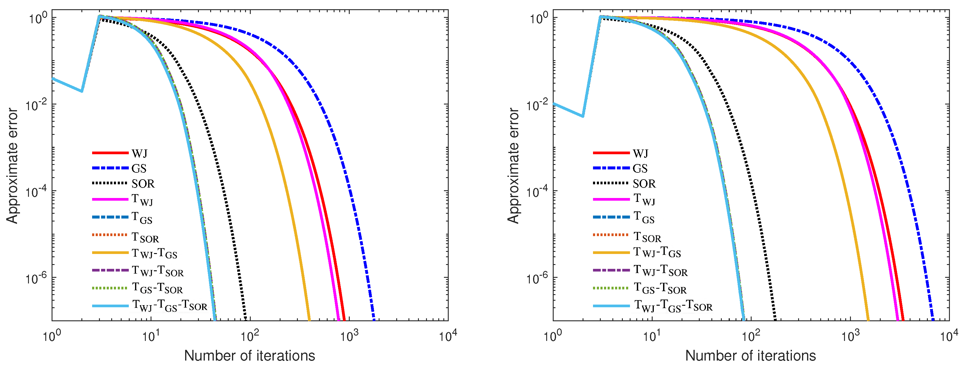
where $\tilde{N}$ is the number of iterations at which we want to stop with ${ϵ}_l={10}^{-7}$. The estimated error per iteration step for all cases was measured by using the relative error $\parallel {\mathbf{u}}_{\mathbf{n}}{-\mathbf{u}\parallel }_2/{\parallel \mathbf{u}\parallel }_2$. Figure 1 shows the estimated error per iteration step for all cases with $l=50$ and $l=100$.

Figure 1. Relative error of the GS, WJ, and SOR methods and all cases of the proposed methods in solving the problem (16) with $l=50$ and $l=100$, respectively.

The trend of the number of iterations for the WJ, GS, and SOR methods and all case studies of the proposed methods in solving the linear system (16) with $l=50$ and $l=100$ is shown in Figure 2.

Figure 2. The progression in the number of iterations for the GS, WJ, and SOR methods and the proposed methods in solving the problem (12)) with $l=50$ and $l=100$, respectively.

Figure 1 and Figure 2 show that the proposed method using $T_{\mathrm{WJ}}$ was better than the WJ method, the proposed method with $T_{\mathrm{GS}}$ was better than the GS method, and the proposed method with $T_{\mathrm{SOR}}$ was better than SOR method when the speed of convergence and the number of iterations are compared. We also found that, when the proposed method with $M>1$ was used (parallel algorithm), the number of iterations was based on the minimum number of iterations used in the nonparallel proposed methods. That is, when the parallel algorithms were used, it can be seen from Figure 2 that the number of iterations of the proposed method with $T_{\mathrm{WJ}}$–$T_{\mathrm{GS}}$ was the same as the proposed method with $T_{\mathrm{GS}}$ and the number of iterations of the proposed method with $T_{\mathrm{WJ}}$–$T_{\mathrm{SOR}}$, $T_{\mathrm{GS}}$–$T_{\mathrm{SOR}}$, $T_{\mathrm{WJ}}$–$T_{\mathrm{GS}}$–$T_{\mathrm{SOR}}$ was the same as the proposed method with $T_{\mathrm{SOR}}$. As a result of the parallel algorithm in which $T_{\mathrm{SOR}}$ was used as its partial components (The proposed methods with $T_{\mathrm{WJ}}$–$T_{\mathrm{SOR}}$, $T_{\mathrm{GS}}$–$T_{\mathrm{SOR}}$, $T_{\mathrm{WJ}}$–$T_{\mathrm{GS}}$–$T_{\mathrm{SOR}}$), this will give us the fastest convergence.

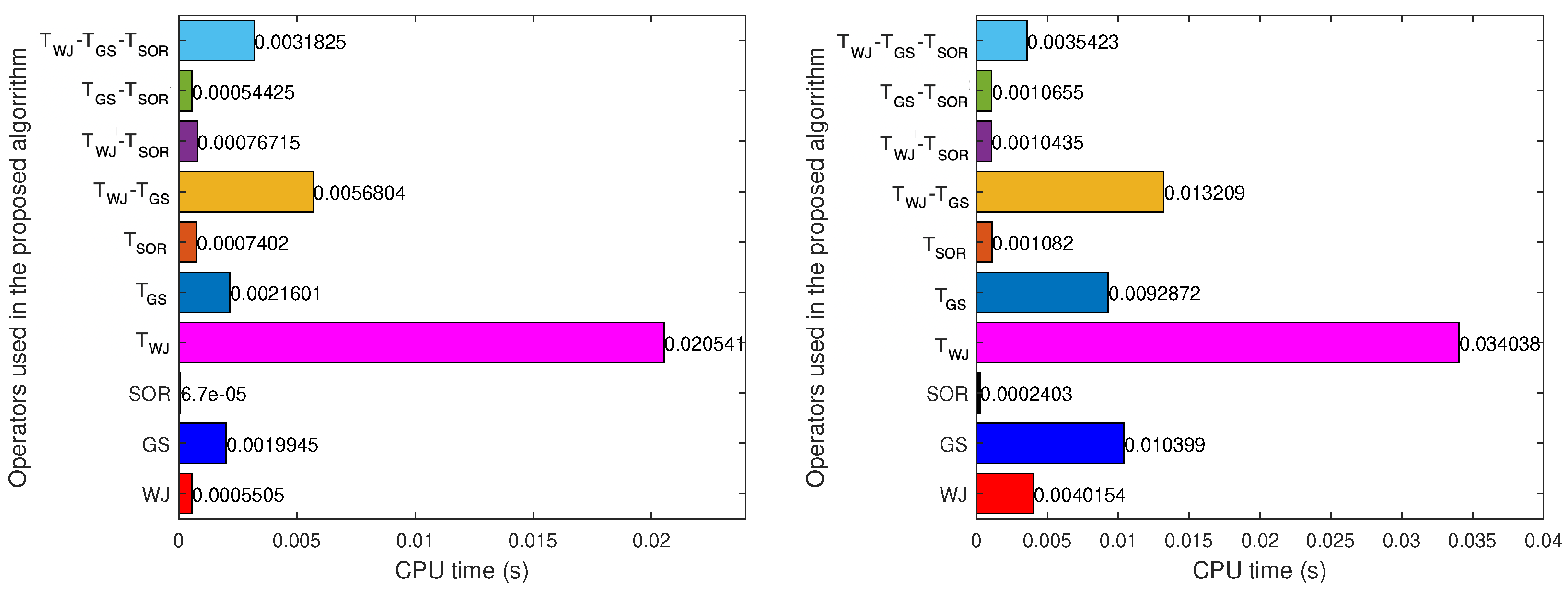
Figure 3 shows that the CPU time of the SOR method was better than the other methods. However, the CPU time of the proposed method using the parallel technique $T_{\mathrm{WJ}}$–$T_{\mathrm{GS}}$–$T_{\mathrm{SOR}}$ was better, close to the SOR method as compared to the other way, when the grid size of matrix A was increased.

Figure 3. The progression of the CPU time for the GS, WJ, and SOR methods and the proposed methods in solving the problem (12) with $l=50$ and $l=100$, respectively.

Next, we provide a comparison of proposed algorithm with the PMHM, HTI, and VAM (where $T_n$ is the $W_n$-mapping, which was introduced by Shimoji and Takahashi [22] with setting ${\alpha }_n=\frac{n}{n+1}$). For the parameter in the HTI and VAM, we chose ${\alpha }_n=\frac{n}{n+1}$. Let $f_n\left(u_n\right)=\frac{u_n}{8}$ in the VAM algorithm and $f_n\left(u_n\right)=0.7u_0$ in the HTI algorithm. The results are reported in Table 3 and Figure 4.

Table 3. The progression of the CPU time for the linear system problem.

$\mathit{l}=50$, $\mathbf{eps}={10}^{-4}$
Algorithm	Proposed	PMHM	HTI	VAM
CPU time	0.0052	0.0072	0.3167	0.8132
$l=100$, $\mathrm{eps}={10}^{-4}$
Algorithm	Proposed	PMHM	HTI	VAM
CPU time	0.0063	0.0074	1.1320	3.5399

Figure 4. The progression of the number of iterations for the proposed methods and the PMHM, HTI, and VAM in solving the problem (12) with $l=50$ and $l=100$, respectively.

From Table 3 and Figure 4, we see that the CPU time and the number of iterations of the proposed algorithm were better than the PMHM, HTI, and VAM.

4.2. Differential Problems

Consider the following simple and well-known periodic heat problem with Dirichlet boundary conditions (DBCs) and initial data:

$$u_t=\vartheta u_{xx}+f(x,t),0<x<l,t>0.$$

$$u(x,0)=u_0\left(x\right),0<x<l,$$

(20)

$$u(0,t)={\psi }_1\left(t\right),u(l,t)={\psi }_2\left(t\right),t>0,$$

where $\vartheta$ is constant, $u(x,t)$ represents the temperature at points $(x,t)$ and $f(x,t)$, and ${\psi }_1\left(t\right)$ and ${\psi }_2\left(t\right)$ are sufficiently smooth functions. Below, we use the notations $u_n^i$ and ${\left(u_{xx}\right)}_n^i$ to represent the approximate numerical values of $u(x_i,t_n)$ and $u_{xx}(x_i,t_n)$, and $t_n=n\Delta t$, where $\vartheta t$ denotes the size of the temporal mesh. The following well-known Crank–Nicolson-type scheme [12,21] is the foundation for a set of schemes used to solve the heat problem (20):

$${\displaystyle {\displaystyle \frac{u_{n+1}^i-u_n^i}{\Delta t}}={\displaystyle \frac{\vartheta }{2}}\left[{\left(u_{xx}\right)}_{n+1}^i+{\left(u_{xx}\right)}_n^i\right]+f_{n+1/2}^i,i=2,\dots ,N-1}$$

(21)

with initial data:

$$u_0^i=u_0\left(x_i\right),i=2,\dots ,N-1$$

(22)

and DBCs:

$$u_{n+1}^1={\psi }_1\left(t_{n+1}\right),u_{n+1}^N={\psi }_2\left(t_{n+1}\right).$$

(23)

To approximate the term of ${\left(u_{xx}\right)}_k^i,k=n,n+1$, we used the standard centered discretization with space. The matrix form of the well-known second-order finite difference scheme (FDS) in solving the heat problem (20) can be written as

$$A{\mathbf{u}}_{n+1}={\mathbf{G}}_n$$

(24)

where ${\mathbf{G}}_n=B{\mathbf{u}}_n+{\mathbf{f}}_{n+1/2}$:

$$A=\left[\begin{array}{ccccc}\hfill 1+\eta & \hfill -{\displaystyle \frac{\eta }{2}}& & & \\ \hfill -{\displaystyle \frac{\eta }{2}}& \hfill 1+\eta & \hfill -{\displaystyle \frac{\eta }{2}}& & \\ & \hfill \ddots & \hfill \ddots & \hfill \ddots & \\ & & \hfill -{\displaystyle \frac{\eta }{2}}& \hfill 1+\eta & \hfill -{\displaystyle \frac{\eta }{2}}\\ & & & \hfill -{\displaystyle \frac{\eta }{2}}& \hfill 1+\eta \end{array}\right],B=\left[\begin{array}{ccccc}\hfill 1-\eta & \hfill {\displaystyle \frac{\eta }{2}}& & & \\ \hfill {\displaystyle \frac{\eta }{2}}& \hfill 1-\eta & \hfill {\displaystyle \frac{\eta }{2}}& & \\ & \hfill \ddots & \hfill \ddots & \hfill \ddots & \\ & & \hfill {\displaystyle \frac{\eta }{2}}& \hfill 1-\eta & \hfill {\displaystyle \frac{\eta }{2}}\\ & & & \hfill {\displaystyle \frac{\eta }{2}}& \hfill 1-\eta \end{array}\right],$$

$${\mathbf{u}}_n=\left[\begin{array}{c}{u}_k^2\\ u_k^3\\ ⋮\\ u_k^{N-2}\\ u_k^{N-1}\end{array}\right],{\mathbf{f}}_{n+1/2}=\left[\begin{array}{c}{\displaystyle \frac{\eta }{2}}{\psi }_{n+1/2}^1+\Delta t{f}_{n+1/2}^2\\ \Delta t{f}_{n+1/2}^3\\ ⋮\\ \Delta t{f}_{n+1/2}^{N-2}\\ {\displaystyle \frac{\eta }{2}}{\psi }_2^{n+1/2}+\Delta t{f}_{n+1/2}^{N-1}\end{array}\right],$$

$\eta =\vartheta \Delta t/\left(\Delta x^2\right)$, ${\gamma }_{n+1/2}^i={\gamma }^i\left(t_{n+1/2}\right),i=1,2$, and $f_{n+1/2}^i=f(x^i,t_{n+1/2})$, $i=2,\dots ,N-1$. According to Equation (24), matrix A is square and symmetrically positive definite. This scheme uses a three-point stencil and reaches the second-order approximation with time and space. The scheme (21) is consistent with the problem (20). The required and sufficient criterion for the stability of the scheme (21) is $\Vert A^{-1}B\Vert \le 1$ (see [12]).

The discretization of the considered problem (24) has traditionally been solved using iterative methods. Here, the well-known WJ and SOR methods were chosen as examples (see Table 4).

Table 4. The specific name of $\mathrm{WJ}$ and $\mathrm{SOR}$ in solving the discretization of the considered problem (24).

Consideration Problem (24)	Iterative Method	Specific Name
$A{\mathbf{u}}_{n+1}={\mathbf{G}}_n$	$D{\mathbf{u}}_{(n+1,s+1)}=\left(D-\omega A\right){\mathbf{u}}_{(n+1,s)}+\omega {\mathbf{G}}_n$	WJ
	$\left(D-\omega L\right){\mathbf{u}}_{(n+1,s+1)}=\left((D-\omega L)-\omega A\right){\mathbf{u}}_{(n+1,s)}+\omega {\mathbf{G}}_n$	SOR

The weight parameter is $\omega$; the diagonal component of matrix A is D; the lower triangular part of matrix $D-A$ is L. Moreover, the optimal weight parameter ${\omega }_o$ is also indicated with the same formula in Table 2. The step sizes of the time play an important role in the stability needed for the WJ and SOR methods in solving the linear systems (24) generated from the discretization of the considered problem (20). The discussion on the stability of the WJ and SOR methods in solving the linear systems (24) can be found in [20,21].

Let us consider the linear system:

$$A\mathbf{u}=\mathbf{G}$$

(25)

where $A:{\mathbb{R}}^l\to {\mathbb{R}}^l$ is a linear and positive operator and $\mathbf{u},\mathbf{G}\in {\mathbb{R}}^l$. We transformed this linear system into the form of a fixed point equation $T\left(\mathbf{u}\right)=\mathbf{u}$ to determine the solution of the linear system (25). For example, the well-known WJ, SOR, and GS approaches present the linear system (25) as a fixed point equation (see Table 5).

Table 5. The alternative method of rearranging the linear systems (25) into the form $\mathbf{u}=T\left(\mathbf{u}\right)$.

Linear System	Fixed Point Mapping $\mathit{T}\left(\mathbf{u}\right)$
$A\mathbf{u}=\mathbf{G}$	$T_{\mathrm{WJ}}\left(\mathbf{u}\right)=\left(I-\omega D^{-1}A\right)\mathbf{u}+\omega D^{-1}\mathbf{G}$
	$T_{\mathrm{GS}}\left(\mathbf{u}\right)=\left(I-{\left(D-L\right)}^{-1}A\right)\mathbf{u}+\omega {\left(D-L\right)}^{-1}\mathbf{G}$
	$T_{\mathrm{SOR}}\left(\mathbf{u}\right)=\left(I-\omega {\left(D-\omega L\right)}^{-1}A\right)\mathbf{u}+\omega {\left(D-\omega L\right)}^{-1}\mathbf{G}$

We introduced a new parallel iterative method using the nonexpansive mapping $T_j,\forall j=1,2,\dots ,M$. Iteratively, the generated sequence $\left\{{\mathbf{u}}_n\right\}$ is created by employing two initial data ${\mathbf{u}}_0={\mathbf{u}}_{(0,1)},{\mathbf{u}}_1={\mathbf{u}}_{(1,1)}\in {\mathbb{R}}^l$ and

$$\begin{array}{cc}\hfill {\mathbf{t}}_{(n,s+1)}& ={\mathbf{u}}_{(n,s+1)}+{\theta }_n\left({\mathbf{u}}_{(n,s+1)}-{\mathbf{u}}_{(n,s)}\right),\hfill \\ \hfill {\mathbf{v}}_{(n,s+1)}^j& ={\alpha }_{n}f\left({\mathbf{t}}_{(n,s+1)}\right)+{\beta }_n{\mathbf{t}}_{(n,s+1)}+{\gamma }_n{T}_j{\mathbf{t}}_{(n,s+1)}\hfill \\ \hfill & +\left(1-({\alpha }_n+{\beta }_n+{\gamma }_n)\right)T_j\circ T_j\left({\mathbf{t}}_{(n,s+1)}\right),j=1,\dots ,M\hfill \\ \hfill {\mathbf{u}}_{(n+1,s+1)}& =\mathrm{argmax}\parallel {\mathbf{v}}_{(n,s+1)}^i-{\mathbf{t}}_{(n,s+1)}\parallel ,n\ge 1,\hfill \end{array}$$

(26)

where the second superscript “s”, $s=1,2,\dots ,{\widehat{S}}_n$, denotes the number of iterations, $\left\{{\alpha }_n\right\},\left\{{\vartheta }_n\right\},\left\{{\gamma }_n\right\}$ are appropriate real sequences in $[0,1]$, and f is a contraction mapping. The following stopping criteria were employed:

$$\parallel {\mathbf{u}}_{(n+1,{\widehat{S}}_n+1)}-{\mathbf{u}}_{(n+1,{\widehat{S}}_n)}{\parallel }_2<{ϵ}_d,$$

where $``{\widehat{S}}_n$” denotes the last iteration at time $t_n$, and then, we set

$${\mathbf{u}}_{(n,1)}={\mathbf{u}}_{(n-1,1)},{\mathbf{u}}_{(n+1,{\widehat{S}}_n+1)}={\mathbf{u}}_{(n,1)}.$$

Next, the proposed method (26) in obtaining the solution of the problem (24) generated from the discretization of the heat problem with DBCs and the initial data (20) was then compared to the well-known WJ, GS, and SOR methods with their optimal parameters. The proposed method (26) with $M\le 3$ and the nonexpansive mapping T chosen from $T_{\mathrm{WJ}},T_{\mathrm{SOR}}$, and $T_{\mathrm{GS}}$ were compared.

Let us consider the simple heat problems:

$$\begin{array}{cc}\hfill & u_t=\vartheta u_{xx}+0.4\vartheta (4{\pi }^2-1)e^{-4\vartheta t}cos\left(4\pi x\right),0\le x\le 1,0<t<t_s,\hfill \\ \hfill & u(x,0)=cos\left(4\pi x\right)/10,u(0,t)=e^{-4\vartheta t}/10,u(1,t)=e^{-4\vartheta t}/10,\hfill \\ \hfill & u(x,t)=e^{-4\vartheta t}cos\left(4\pi x\right)/10.\hfill \end{array}$$

(27)

The results of the WJ, GS, and SOR methods were compared with all case studies of the proposed methods, which is the same as Section 4.1. Because we focused on the convergence of the proposed method, the stability analysis in selecting the time step sizes is not described in depth. The proposed methods’ time step size was based on the least step size selected from the WJ and SOR methods in solving the problem (24) obtained from the discretization of the considered problem (27).

All computations were carried out on a uniform grid of N nodes, which corresponds to the solution of the problem (24) with $N-2\times N-2$ sizes of matrix A and $\Delta x=1/(N-1)$. The weight parameter $\omega$ of the proposed method is defined as the optimum weight parameter ($\omega o$) in Table 2.

We used $\vartheta =25$, $\Delta t=\Delta x^2/10$, ${ϵ}_d={10}^{-7}$, the default parameters ${\alpha }_n,{\beta }_n,{\gamma }_n$, and the function f set as Equations (17)–(19) and

$${\theta }_n=\left\{\begin{array}{cc}{\displaystyle min\left\{{\displaystyle \frac{1}{n^2{\parallel {\mathbf{u}}_n-{\mathbf{u}}_{n-1}\parallel }_2}},0.121\right\}}\hfill & \mathrm{if}{\mathbf{u}}_{\mathrm{n}}\ne {\mathbf{u}}_{\mathrm{n}-1},\hfill \\ {\displaystyle 0.121}\hfill & \mathrm{otherwise},\hfill \end{array}\right.$$

(28)

where $\tilde{N}$ is the number of iterations at which we want to stop. For testing purposes only, all computations were carried out for $0\le t\le 0.01$ (when $t\gg 0.05,u(x,t)\to 0$). Figure 5 shows the approximate solution of the problem (27) with 101 nodes at $t=0.01$ by using the WJ, GS, and SOR methods and the proposed methods.

Figure 5. Approximate solutions of the GS, WJ, and SOR methods and all cases of the proposed methods in solving the problem (27) with 101 nodes.

It can be seen from Figure 5 that all numerical solutions matched the analytical solution reasonably well. Figure 6 shows the trend of the iteration number for the WJ, GS, and SOR methods and the proposed methods in solving the problem (24) generated from the discretization of the considered problem (27) with 101 nodes. It was found that the proposed method with $T_{\mathrm{WJ}}$ was better than the WJ method, the proposed method with $T_{\mathrm{GS}}$ was better than the GS method, and the proposed method with $T_{\mathrm{SOR}}$ was better than the SOR method when the number of iterations was compared.

Figure 6. The evolution of the number of iterations for the WJ, GS, and SOR methods and the proposed methods in solving the problem (20) with 101 nodes and $t\in (0,1]$.

We see that the number of iterations of the proposed method with $0<n\le 3$ depends on the minimum number of iterations of the nonparallel proposed methods used. That is, the number of iterations of the proposed method at each time step with $T_{\mathrm{WJ}}$–$T_{\mathrm{GS}}$ was the same as the proposed method with $T_{\mathrm{GS}}$, and the number of iterations at each time step of the proposed methods with $T_{\mathrm{WJ}}$–$T_{\mathrm{SOR}}$, $T_{\mathrm{GS}}$–$T_{\mathrm{SOR}}$, and $T_{\mathrm{WJ}}$–$T_{\mathrm{GS}}$–$T_{\mathrm{SOR}}$ was the same as the proposed method with $T_{\mathrm{SOR}}$.

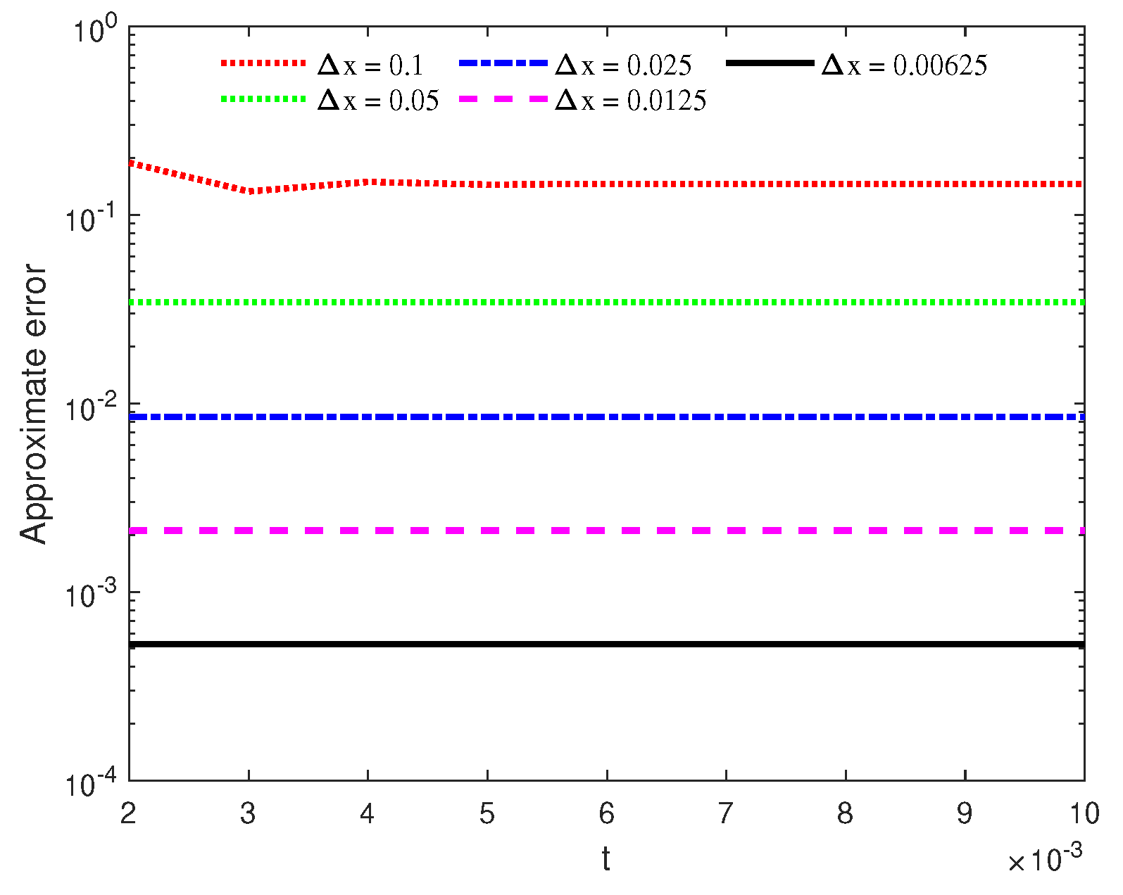
Next, the proposed method with $T_{\mathrm{WJ}}$–$T_{\mathrm{GS}}$–$T_{\mathrm{SOR}}$ was chosen in solving the problem (24) generated from the discretization of the considered problem (27) to test and verify the order of accuracy for the presented FDS in solving the heat problem. All computations were carried out on uniform grids of 11, 21, 41, 81, and 161 nodes, which correspond to the solution of the discretization of the heat problem (27) with $\Delta x$ = 0.1, 0.05, 0.025, 0.0125, and 0.0625, respectively. The evolution of their relative error $\parallel {\mathbf{u}}_{\mathbf{n}}{-\mathbf{u}\parallel }_2/{\parallel \mathbf{u}\parallel }_2$ at each time step reached under the acceptable tolerance ${ϵ}_d=1\times {10}^{-7}$ for the numerical solution of the heat problem problem with various grid sizes is shown in Figure 7.

Figure 7. The evolution of the relative error in obtain the numerical solution of the problem (27) with various grid sizes by using the proposed method with $T_{\mathrm{WJ}}$–$T_{\mathrm{GS}}$–$T_{\mathrm{SOR}}$.

When the distance between the graphs of all computational grid sizes was examined, the proposed method using $T_{\mathrm{WJ}}$–$T_{\mathrm{GS}}$–$T_{\mathrm{SOR}}$ was shown to have second-order accuracy. That is, the order of the accuracy of the proposed method using $T_{\mathrm{WJ}}$–$T_{\mathrm{GS}}$–$T_{\mathrm{SOR}}$ corresponds to the FDS construction. Figure 8 shows the trend of the iteration number for the WJ, GS, and SOR methods compared with all cases of the proposed methods in solving the discretization of the considered problem (27) with varying grid sizes.

Figure 8. The evolution of the iteration number for the GS, WJ, and SOR methods and the proposed methods in solving the problem (20) with $\vartheta =25$ and $t\in (0,1]$.

It can be seen that, when the grid size was small, the parallel algorithm in which the $T_{\mathrm{GS}}$ or $T_{\mathrm{SOR}}$ was used as its partial components gave us the lowest number of iterations under the accepted tolerance.

From Figure 9, we see that the CPU time of the SOR method was better than the other methods. However, the CPU time of the proposed method using the parallel technique $T_{\mathrm{WJ}}$–$T_{\mathrm{GS}}$–$T_{\mathrm{SOR}}$ was better, close to the SOR method as compared to the other way, when the grid size of matrix A was increased.

Figure 9. The evolution of the CPU time for the GS, WJ, and SOR methods and the proposed method in solving problem (20) with $\vartheta =25$ and $t\in (0,1]$.

Next, we provide a comparison of the proposed algorithm with the PMHM, HTI, and VAM (where $T_n$ is a $W_n-$ mapping, which was introduced by Shimoji and Takahashi [22] with setting ${\alpha }_n=\frac{n}{n+1}$). As the parameter in the HTI and VAM, we chose ${\alpha }_n=\frac{n}{n+1}$. Let $f_n\left(u_n\right)=\frac{u_n}{8}$ in the VAM algorithm and $f_n\left(u_n\right)=0.7u_0$ in the HTI algorithm. The results are reported in Figure 10 and Figure 11.

Figure 10. The average number of iterations for the proposed methods and the PMHM, HTI, and VAM.

Figure 11. The CPU time for the proposed methods and the PMHM, HTI, and VAM.

From Figure 10 and Figure 11, we see that the CPU time and number of iterations of the proposed algorithm were better than the PMHM, HTI, and VAM.

Moreover, the our method can solve many real-word problems such as image and signal processing, optimal control, regression, and classification problems by setting $T_i$ as the proximal gradient operator. Therefore, we present the examples of the signal recovery in the next.

4.3. Signal Recovery

In this part, we present some numerical examples of the signal recovery by the proposed methods. A signal recovery problem can be modeled as the following underdetermined linear equation system:

$$b=Au+ϵ,$$

(29)

where $u\in {\mathbb{R}}^N$ is the original signal and $b\in {\mathbb{R}}^M$ is the observed signal, which is squashed by the filter matrix $A:{\mathbb{R}}^N\to {\mathbb{R}}^M$ and noise $ϵ$. It is well known that the problem (29) can be solved by the LASSO problem:

$${\displaystyle \underset{u\in {\mathbb{R}}^N}{min}\frac{1}{2}{\parallel b-Au\parallel }_2^2+\lambda {\parallel u\parallel }_1,}$$

(30)

where $\lambda >0$. As a result, various techniques and iterative schemes have been developed over the years to solve the LASSO problem; see [15,16]. In this case, we set $T{u}_n={\mathrm{prox}}_{\lambda g}(u_n-\lambda \nabla f\left(u_n\right))$, where $f\left(u\right)=\frac{1}{2}{\parallel b-Au\parallel }_2^2$ and $g\left(u\right)={\lambda \parallel u\parallel }_1$. It is known that T is a nonexpansive mapping when $\lambda \in (0,2/L)$, and L is the Lipschitz constant of $\nabla f$.

The goal in this paper was to remove noise without knowing the type of filter and noise. Thus, we are interested in the following problem:

$$\begin{array}{c}\hfill \begin{array}{ccc}\hfill {\displaystyle \underset{u\in {\mathbb{R}}^N}{min}\frac{1}{2}{\parallel A_{1}u-b_1\parallel }_2^2}& +\hfill & \hfill {\lambda }_1{\parallel u\parallel }_1,\\ \hfill {\displaystyle \underset{u\in {\mathbb{R}}^N}{min}\frac{1}{2}{\parallel A_{2}u-b_2\parallel }_2^2}& +\hfill & \hfill {\lambda }_2{\parallel u\parallel }_1,\\ & ⋮\hfill & \\ \hfill {\displaystyle \underset{u\in {\mathbb{R}}^N}{min}\frac{1}{2}{\parallel A_{N}u-b_N\parallel }_2^2}& +\hfill & \hfill {\lambda }_N{\parallel u\parallel }_1.\end{array}\end{array}$$

(31)

where u is the original signal, $A_i$ is a bounded linear operator, and $b_i$ is an observed signal with noise for all $i=1,2,...,N.$

We can apply Algorithm 1 to solve the problem (31) by setting $T_i{u}_n={\mathrm{prox}}_{{\lambda }_i{g}_i}$$(u_n-{\lambda }_i\nabla f_i\left(u_n\right))$.

In our experiment, the sparse vector $u\in {\mathbb{R}}^N$ was generated by the uniform distribution in [−2, 2] with n nonzero elements. $b_1,$$b_2,$$b_3$ were generated by the normal distribution matrix $A_1,A_2,A_3\in {\mathbb{R}}^{M\times N}$, respectively, with white Gaussian noise such that the signal-to-noise ratio (SNR) = 40. The initial point $u_1$ was picked randomly. We used the mean-squared error (MSE) for estimating the restoration accuracy, which is defined as follows:

$$\mathrm{MSE}=\frac{1}{N}{\parallel u_n-u_{*}\parallel }_2^2<{10}^{-4},$$

where $u_{*}$ is the estimated signal of u.

In what follows, let the step size parameter ${\lambda }_i={\displaystyle \frac{1.999}{{max}_{1\le i\le 3}(\parallel A_i{\parallel }^2)}}$ for all $i=1,2,3$, when the contraction mapping $f:H\to H$ is defined by $f\left(x\right)=0.9x,\forall x\in H$. We study the convergence behavior of the sequence ${\theta }_n$ when

$$\begin{array}{c}\hfill {\theta }_n=\left\{\begin{array}{cc}{\epsilon }_n,\hfill & \mathrm{if}n\le K\mathrm{and}{u}_n\ne u_{n-1}\hfill \\ \frac{{\alpha }_n}{n^2\parallel u_n-u_{n-1}\parallel },\hfill & \mathrm{if}n>K\mathrm{and}{u}_n\ne u_{n-1}\hfill \\ 0.4,\hfill & \mathrm{if}\mathrm{otherwise},\hfill \end{array}\right.\end{array}$$

(32)

where K is the number of iterations at which we want to stop.

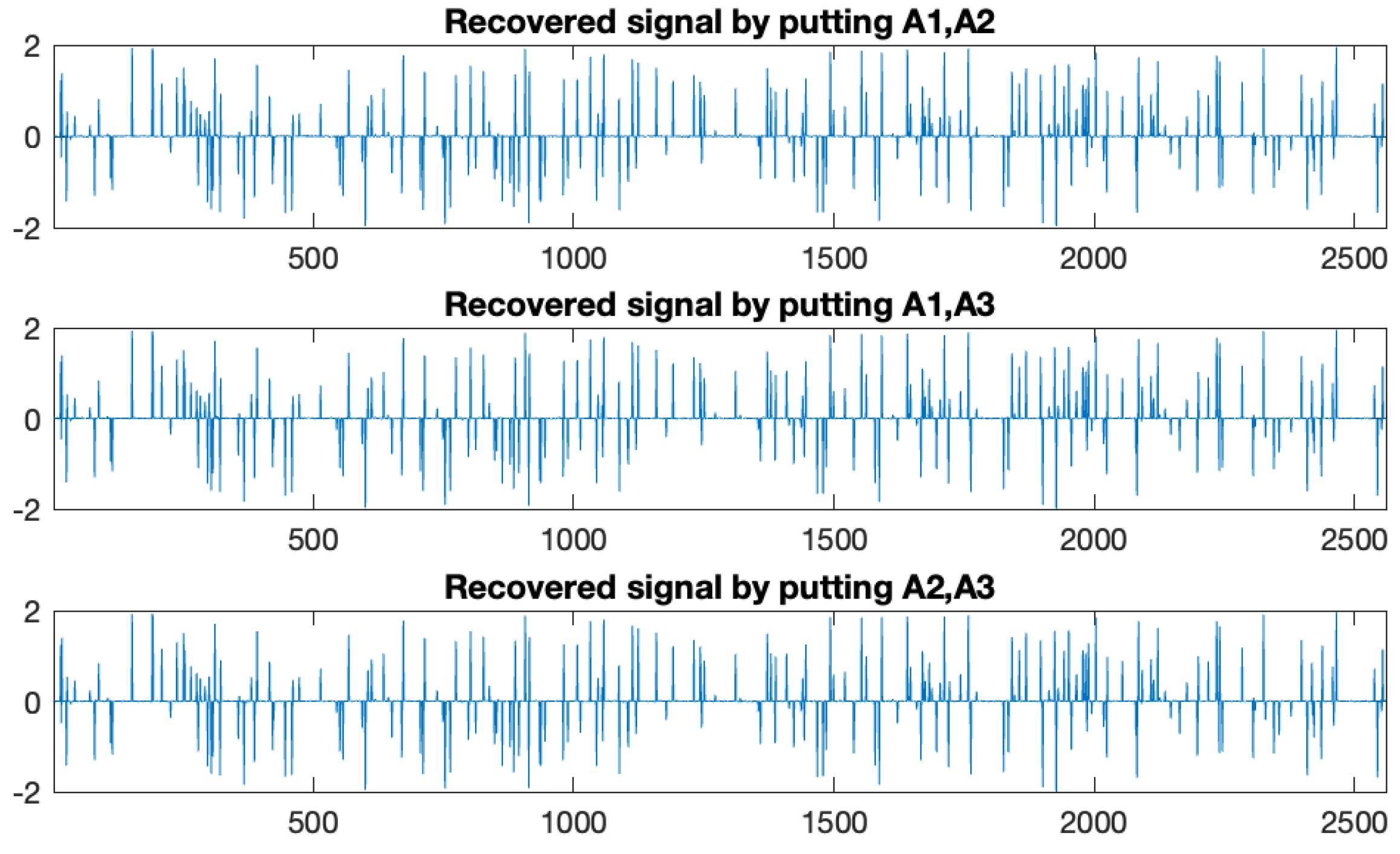
The iterative scheme was varied by choosing different ${\epsilon }_n$ in the following cases:

Case 1.

${\epsilon }_n=0$;

Case 2.

${\epsilon }_n=min(0.13,{\displaystyle \frac{1}{\parallel u_1-u_0\parallel }})$;

Case 3.

${\epsilon }_n=min(0.45,{\displaystyle \frac{1}{\parallel u_1-u_0\parallel }})$;

Case 4.

${\epsilon }_n=min(0.87,{\displaystyle \frac{1}{\parallel u_1-u_0\parallel }})$;

Case 5.

${\epsilon }_n=0.45$;

Case 6.

${\epsilon }_n=0.89$.

We set the number of iterations at which we wanted to stop $K=$ 10,000, and in all cases, we set ${\alpha }_n=\frac{1}{5n+1}$, ${\beta }_n=0.3$, and ${\gamma }_n={\beta }_n$. The results are reported in Table 6.

Table 6. The convergence of Algorithm 1 with each ${\epsilon }_n$ for parameter ${\theta }_n$.

Parameter ${\mathit{\theta }}_{\mathit{n}}$		Case 1	Case 2	Case 3	Case 4	Case 5	Case 6
A1	CUP	7.3927	7.0153	4.2289	1.8295	5.3543	3.0668
	Iter	3830	3661	2076	451	2684	1402
A2	CUP	7.5717	6.5441	3.8712	1.3047	5.4360	2.9778
	Iter	3993	3436	1902	438	2762	1419
A3	CUP	7.4972	6.6584	4.0925	1.3244	5.4799	3.3457
	Iter	4009	3509	1971	453	2836	1447
A1A2	CUP	2.9380	2.5944	2.0119	1.3225	2.5928	2.1553
	Iter	499	402	259	73	410	259
A1A3	CUP	2.8789	2.7574	1.9361	1.3796	2.5989	2.3089
	Iter	475	459	248	76	409	249
A2A3	CUP	2.9561	2.7747	2.1093	1.333	2.6121	2,1656
	Iter	503	447	278	77	394	231
A1A2A3	CUP	19907	1.9641	1,7686	1.7525	1.8102	3.2931
	Iter	74	68	41	37	45	171

From Table 6, it is shown that the parameter $\theta$ depends on ${\epsilon }_n=0$ using the number of iterations with the CPU time of our algorithm more than the other ${\epsilon }_n$. Furthermore, we see that the case of inputting had a lower number of iterations and CPU time than the case of inputting $AiAi,i=1,2$ and $Ai,i=1,2,3$ for all of the cases. This means that the efficiency of the proposed algorithm is better when the number of subproblems is increasing.

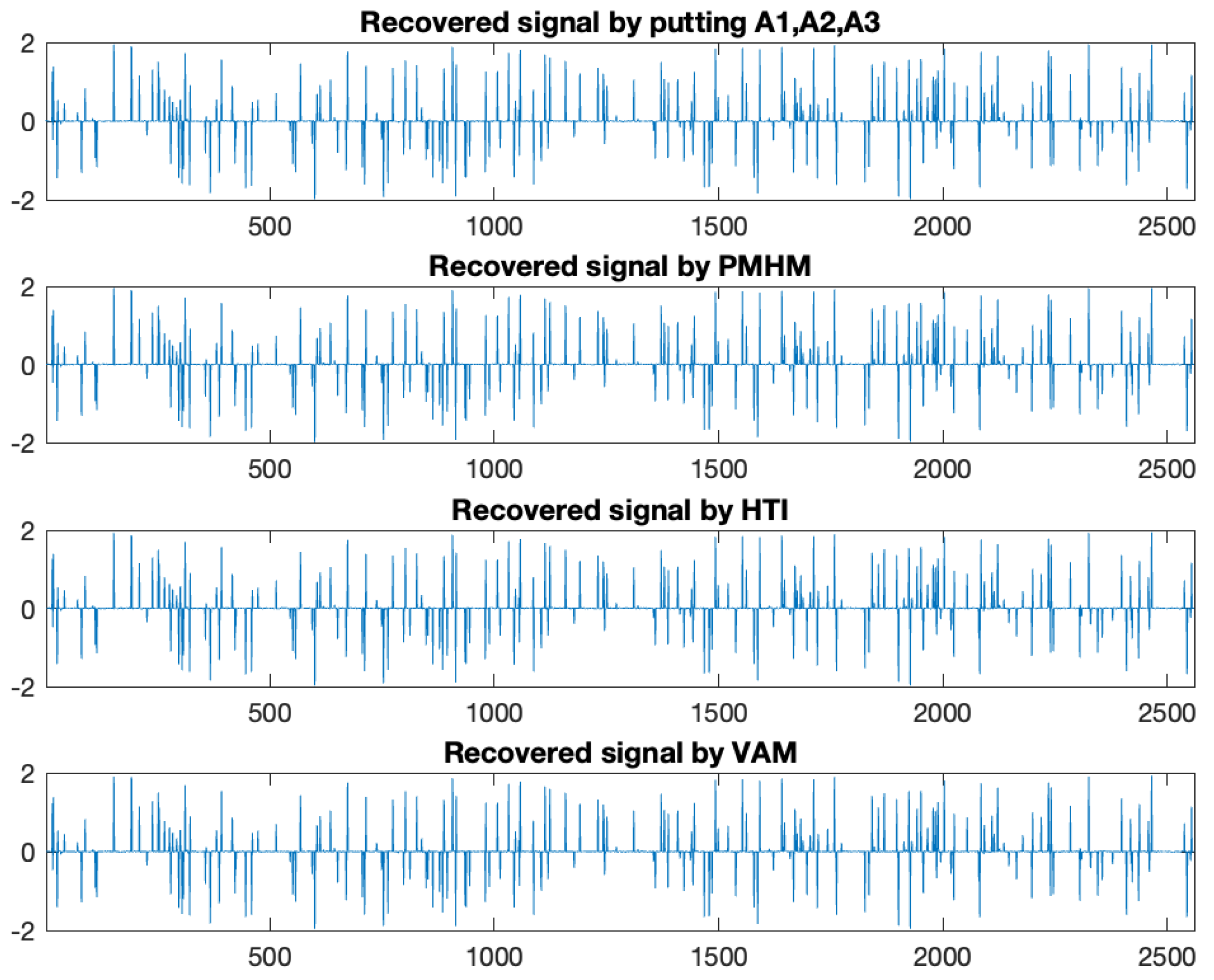
Next, we provide a comparison of the proposed algorithm with the PMHM, HTI, and VAM (where $T_n$ is a $W_n$-mapping, which was introduced by Shimoji and Takahashi [22] with setting ${\alpha }_n=\frac{n}{n+1}$). We set the parameter in the PMHM algorithm as ${\alpha }_n=1-\frac{n}{n+1}$. The parameter in the HTI and VAM was chosen as ${\alpha }_n=\frac{n}{n+1}$ and ${\beta }_n=\frac{n}{n+1}$. Let $f_n\left(u_n\right)=\frac{u_n}{8}$ in the VAM algorithm and $f_n\left(u_n\right)=0.7u_0$ in the HTI algorithm. We plot the number of iterations versus the mean-squared error (MSE) and the original signal, observation data, and recovered signal for one case with $N=2560,M=1280$, and $m=210$. The results are reported in Table 7.

Table 7. The computational results for solving the LASSO problem.

		$\mathit{N}=2560,$$\mathit{M}=1280$
		$\mathit{m}=\mathbf{210}$	$\mathit{m}=\mathbf{230}$	$\mathit{m}=\mathbf{250}$
A1	CUP	1.3953	1.4232	1.6346
	Iter	443	449	503
A2	CUP	1.3978	1.4164	1.5908
	Iter	440	474	474
A3	CUP	1.2974	1.2871	1.3930
	Iter	411	419	427
A1A2	CUP	1.3888	1.4732	1.5538
	Iter	75	75	78
A1A3	CUP	1.4487	1.3061	1.3578
	Iter	72	70	82
A2A3	CUP	1.3728	1.2877	1.2515
	Iter	73	68	75
A1A2A3	CUP	1.7252	1.8706	1.8094
	Iter	37	38	37
PMHM	CUP	2.6205	2.7398	2.4789
	Iter	252	262	264
HTI	CUP	2.0454	2.0043	2.0365
	Iter	121	127	130
VAM	CUP	1.7917	2.2685	2.0194
	Iter	58	64	60

From Table 7, we see by the MSE values that our algorithm using the parallel method was faster than the PMHM, HTI, and VAM in terms of the number of iterations and the CPU time.

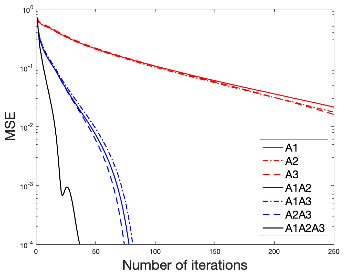
From Figure 12, it is shown that the MSE value of Algorithm 1 with $A1A2A3$ decreased faster than that of Algorithm 1 with $A_i{A}_i,i=1,2$, and that with $A_i{A}_i,i=1,2$ decreased faster than that of Algorithm 1 with $A_i,i=1,2,3$.

Figure 12. The graphs of the MSE for Algorithm 1 with the input $A_i,$$i=1,2,3$.

The original signal, observation data, and recovered signal are shown in Figure 13, Figure 14, Figure 15 and Figure 16.

Figure 13. The original signal size $N=2560,M=1280$, and 250 spikes and the measured values with $A_i,i=1,2,3$, SNR = 40, respectively.

Figure 14. The recovered signal with $m=210$ by A1 (503 Iter, CPU = 1.6346), A2 (474 Iter, CPU = 1.5908), and A3 (427 Iter, CPU = 1.3930), respectively.

Figure 15. The recovered signal with $m=210$ by A1A2 (78 Iter, CPU = 1.5538), A1A3 (82 Iter, CPU = 1.3578), and A2A3 (75 Iter, CPU = 1.2515), respectively.

Figure 16. The recovered signal with $m=210$ by A1A2A3 (37 Iter, CPU = 1.8094), PMHM (264 Iter, CPU = 2.4789), HTI (130 Iter, CPU = 2.0365), and VAM (60 Iter, CPU = 2.0194), respectively.

From Figure 16 and Figure 17, it is shown that Algorithm 1 with A1A2A3 converged faster than the PMHM, HTI, and VAM.

Figure 17. The graphs of the MSE for Algorithm 1 with A1A2A3 and the PMHM algorithm, respectively.

5. Conclusions

In this work, we introduced a viscosity modification combined with the parallel monotone algorithm for a finite family of nonexpansive mappings. We also established a strong convergence theorem. We provided numerical experiments of our algorithm for solving linear system problems and differential problems and showed the efficiency of the proposed algorithm. In the signal recovery problem, it was found that our algorithm had a better convergence behavior than the other algorithms. In the future, the proposed algorithm can be executed to solve a generalized nonexpansive mapping and be applied to solve many real-word problems such as image and signal processing, optimal control, regression, and classification problems.