Power Families of Bivariate Proportional Hazard Models

Abstract

In this paper, we propose a general class of bivariate proportional hazard distributions, which is based on the family of asymmetric proportional hazard distributions and the bivariate Pareto copula. Distributional properties of the bivariate proportional hazard distribution are derived. We specialize the bivariate proportional hazard family of distributions to the normal case, and so we introduce the bivariate proportional hazard normal distribution. Parameter estimation by the maximum likelihood method of the bivariate proportional hazard normal distribution is then discussed. Finally, an application of the new bivariate distribution to real data is considered for illustrative purposes.

1. Introduction

The proportional hazard distribution was presented as an extension of the distribution of the minimum of a random sample replacing $n\in \mathbb{Z}$ with $b>0$ in a random variable Z with probability density function (PDF) f, and cumulative distribution function (CDF) F. So, this distribution could be considered as a distribution of fractional order statistics ([1]). Here, we start defining the proportional hazard (PHF) distribution, which was studied by [2]; see also [3] where inference under progressively type II right-censored sampling for the PHF distribution is considered. Let F be a continuous CDF with PDF $f=dF$, and hazard function $h=f/(1-F).$ We say that Z has a PHF distribution associated with F and f, if its PDF is of the form

$${\phi }_F\left(z\right)=\beta f\left(z\right){\{1-F\left(z\right)\}}^{\beta -1},z\in \mathbb{R},$$

(1)

where $\beta >0$ is the shape parameter. We use the notation $Z\sim \mathrm{PHF}\left(\beta \right)$ to refer to this distribution. The CDF of the PHF distribution is given by

$$\mathbb{F}\left(z\right)=1-{\{1-F\left(z\right)\}}^{\beta },z\in \mathbb{R}.$$

(2)

The hazard function of this model is $h_F\left(z\right)=\beta f\left(z\right)/\{1-F\left(z\right)\}$; that is, the proportional hazard function of the PDF f. From Equation (2), we can use the inversion method for generating a random variable with PHF distribution; that is, if $U\sim \mathcal{U}(0,1)$, i.e., a uniform distribution on the interval $(0,1)$, then the random variable $X=\mu +\sigma F^{-1}(1-{(1-U)}^{1/\beta })$ is distributed according to the PHF distribution with parameter vector $\mathit{\theta }={(\mu ,\sigma ,\beta )}^{\prime }$, where $F^{-1}(·)$ denotes the inverse of $F(·)$. The distributional properties of the PHF distribution, as well as inferential procedures and information matrix for the model parameters are studied by [2].

The location-scale extension of model (1) is obtained using the linear transformation $X=\mu +\sigma Z$, where $\mu \in \mathbb{R}$ is a location parameter, $\sigma >0$ is a scale parameter, and $Z\sim \mathrm{PHF}\left(\beta \right)$. The PDF of the random variable X is given by

$$\phi \left(x\right)=\frac{\beta }{\sigma }f\left(\frac{x-\mu }{\sigma }\right){\left(1-F\left(\frac{x-\mu }{\sigma }\right)\right)}^{\beta -1},x\in \mathbb{R}.$$

(3)

If a random variable X follows the model (3), it is denoted by $X\sim \mathrm{PHF}(\mu ,\sigma ,\beta )$. If $f=\varphi$ and $F=\mathsf{\Phi }$, where $\varphi$ and $\mathsf{\Phi }$ detone the PDF and CDF of a standard normal distribution, we write $X\sim \mathrm{PHN}(\mu ,\sigma ,\beta )$, and so we obtain the proportional hazard normal (PHN) distribution. Note that $\mathrm{PHN}(\mu ,\sigma ,\beta =1)\equiv \mathcal{N}(\mu ,\sigma )$, and so the normal distribution is a special case of the PHN distribution. Hence, it is more flexible than the normal model in terms of skewness and kurtosis, due to the inclusion of the shape parameter $\beta$. We have that the Kumaraswamy-G (KwG) distribution, proposed by [4], is defined by the PDF

$${\phi }_G\left(z\right)=abg\left(z\right)G^{a-1}\left(z\right){\{1-G^a\left(z\right)\}}^{b-1},z\in \mathbb{R},$$

(4)

where G is an arbitrary continuous CDF, and $g=dG$. Also, $a>0$ and $b>0$ are additional shape parameters to that of G. If Z is a random variable with PDF (4), we write $Z\sim \mathrm{KwG}(a,b)$. It is worth stressing that when $a=1$, we obtain the $\mathrm{PHF}\left(b\right)$ distribution, i.e., $\mathrm{KwG}(a=1,b)\equiv \mathrm{PHF}\left(b\right)$, and so this kind of distribution arises as a possible solution when we have asymmetric data.

The construction of multivariate distributions from copula theory can be carried out using the Sklar’s theorem. The way to obtain a multivariate distribution from the Sklar’s theorem is as follows: Let $X_1,\dots ,X_p$ be p random variables with continuous CDFs $F_{X_1}\left(x_1\right),\dots ,F_{X_p}\left(x_p\right),$ respectively. Then, according to Sklar’s theorem, $F_{X_1,\dots ,X_p}(x_1,\dots ,x_p)$ has a unique copula representation:

$$F_{X_1,\dots ,X_p}(x_1,\dots ,x_p)=C(F_{X_1}\left(x_1\right),\dots ,F_{X_p}\left(x_p\right)).$$

Moreover, it is well known that many dependence properties of a multivariate distribution depend only on the corresponding copula. Therefore, many dependence properties of a multivariate distribution can be obtained by studying the corresponding copula. By using Clayton copula, Ref [5] proposed a bivariate extension of the power-normal distribution. Specifically, a bivariate random variable $(X_1,X_2)$ has a bivariate power-normal distribution, denoted by $\mathrm{BPN}(\delta ,{\beta }_1,{\beta }_2)$, if for ${\beta }_1>0$ and ${\beta }_2>0,$ $(X_1,X_2)$ has the following joint CDF

$$F_{X_1,X_2}(x_1,x_2)={({\left\{\mathsf{\Phi }\left(x_1\right)\right\}}^{-{\beta }_1/\delta }+{\left\{\mathsf{\Phi }\left(x_2\right)\right\}}^{-{\beta }_2/\delta }-1)}^{-\delta },(x_1,x_2)\in {\mathbb{R}}^2,$$

where $\delta >0$ is the parameter that controls the dependence in the Clayton copula. The Clayton copula is usually attributed to [6], but it has also been studied by [7]. For $(u,v)\in [0,1]\times [0,1]$, it is defined as

$$C_{\delta }(u,v)={(u^{-1/\delta }+v^{-1/\delta }-1)}^{-\delta },\delta >0.$$

The first systematic study of this model was conducted by [8], who interpreted the parameter $\delta$ as a measure of the dependence between u and $v.$ Therefore, the independence between the variables is obtained when $\delta$ tends to zero. Obviously there are other forms of constructing multivariate distributions, and so new multitariate distributions have been proposed in the statistical literature. To mention a few, but not limited to, we refer the reader to the works by [9,10,11,12], among others.

It is worth emphasizing that the univariate PHF family of distributions has received significant attention over the last years in the statistical literature, mainly due to its flexibility in considering different models in its construction given by f and F; see expression (1). On the other hand, multivariate extensions of this univariate family of distributions has been little explored. This paper fills this gap and provides a bivariate extension of this univariate distribution. The bivariate PHF distribution is quite simple and, hence, may be widely applied in analyzing bivariate real data in practice. Additionally, distributional properties of the bivariate PHF distribution are investigated in details. An important claim to introduce the bivariate PHF distribution relies on the fact that the practitioners will have new bivariate model to use in bivariate settings. Additionally, the formulae related with the new bivariate model are manageable and with the use of modern computer resources and its numerical capabilities, the bivariate PHF distribution may prove to be an useful addition to the arsenal of applied statisticians. We hope that the bivariate distribution introduced in this paper may serve as an alternative bivariate model to some well-known bivariate model available in the statistical literature. We also hope that the bivariate PHF distribution may work better (at least in terms of model fitting) than some bivariate distributions available in the literature in certain practical situations, although it cannot always be guaranteed. Here, the bivariate PHF family of distributions we introduce is obtained from a multivariate distribution which was constructed from Pareto copula (descried in the next section) coupled with PHF marginals. It is worth stressing that many types of copulas are available o construct multivariate distributions, namely: Clayton copula, Frank copula, Joe copula, and Gumbel copula, among others. Perhaps, the most common copula is the Clayton copula. In this paper, instead, we shall consider the Pareto copula to introduce the new bivariate model due to its simplicity and interesting properties (descried in the next section). In addition, the Pareto copula yields a simple form of the likelihood function, so it makes the estimation of the model parameters easy to deal with. In short, it is evident that few works about bivariate generalizations of the PHF distribution have been published in the statistical literature and, hence, a new, simple and tractable bivariate PHF extension of the univariate PHF distribution through Pareto copula is welcome.

The paper is organized as follows. Section 2 presents the Pareto copula and discusses with details the structural properties derived from it. The bivariate proportional hazard distribution is proposed in Section 3. Distributional properties of this bivariate family of distributions are also derived in this section. In Section 4, we study the bivariate PHN distribution, where the univariate normal distribution is taken into account. Location-scale extension, as well as parameter estimation for the bivariate PHN distribution are also discussed in this section. An empirical appliction of the bivariate PHN distribution that considers real data is provided in Section 5 for illustrative purposes. Finally, Section 6 concludes the paper.

2. Pareto Copula

The Pareto distribution, or Pareto type I distribution, has been extensively used in economic literature and in reliability theory. Its CDF is given by

$$G_X\left(x\right)=1-{\left(\frac{x}{\sigma }\right)}^{-\alpha },x>0,$$

where $\sigma >0$ and $\alpha >0$. Another type of Pareto distribution is the Pareto type II distribution, whose CDF takes the form

$$F_X\left(x\right)=1-{\left(1+\frac{x}{\sigma }\right)}^{-\alpha },x>0.$$

Its survival function is given by

$$S_X\left(x\right)={\left(1+\frac{x}{\sigma }\right)}^{-\alpha },x>0.$$

The bivariate Pareto distribution of the random vector $X=(X_1,X_2)$ has joint CDF in the form

$$\begin{array}{cc}\hfill F_{X_1,X_2}(x_1,x_2)& =F_{X_1}\left(x_1\right)+F_{X_2}\left(x_2\right)-1\hfill \\ \hfill & +{[{\left\{S_{X_1}\left(x_1\right)\right\}}^{-1/\alpha }+{\left\{S_{X_2}\left(x_2\right)\right\}}^{-1/\alpha }-1]}^{-\alpha },\hfill \end{array}$$

where $(x_1,x_2)\in {\mathbb{R}}_{+}^2$. Then, using the Sklar’s theorem for continuous marginal distributions, the bivariate Pareto copula is given by

$$\begin{array}{cc}\hfill C(u_1,u_2)& =F_{X_1,X_2}(F_{X_1}^{-1}\left(u_1\right),F_{X_2}^{-1}\left(u_2\right))\hfill \\ \hfill & =u_1+u_2-1+{[{(1-u_1)}^{-1/\alpha }+{(1-u_2)}^{-1/\alpha }-1]}^{-\alpha }.\hfill \end{array}$$

Next, we shall consider some properties of the bivariate Pareto copula:

1.

The joint PDF of the Pareto copula is

$$c(u_1,u_2)=\frac{{\partial }^{2}C(u_1,u_2)}{\partial u_1\partial u_2}=\frac{\alpha +1}{\alpha }\frac{{\left[(1-u_1)(1-u_2)\right]}^{-\frac{\alpha +1}{\alpha }}}{{[{(1-u_1)}^{-1/\alpha }+{(1-u_2)}^{-1/\alpha }-1]}^{\alpha +2}}.$$

2.

The joint survival function of the Pareto copula is

$$S(u_1,u_2)=P(U_1\ge u_1,U_2\ge u_2)={[{(1-u_1)}^{-1/\alpha }+{(1-u_2)}^{-1/\alpha }-1]}^{-\alpha }.$$

3.

For all $u_2\in [0,1],$ the bivariate Pareto copula is a concave function on $u_1$ for fixed $u_2$. This result follows from

$$\frac{{\partial }^{2}C(u_1,u_2)}{\partial u_1^2}=\frac{\alpha +1}{\alpha }\frac{{(1-u_1)}^{-\frac{2\alpha +1}{\alpha }}}{{[{(1-u_1)}^{-1/\alpha }+{(1-u_2)}^{-1/\alpha }-1]}^{\alpha +2}}\ge 0.$$

4.

The bivariate dependency measures for continuous variables, usually used in copulas, are Kendall’s tau correlation coefficient ($\tau$), Spearman’s rho (${\rho }_s$), and the medial correlation coefficient. The first two coefficients are invariant to increasing transformations. The Kendall’s tau measures the difference between the probability of two concordant random pairs and the probability of two discordant random pairs. For a continuous bivariate distribution function F, $\tau$ is defined by

$$\tau =4\int FdF-1.$$

Spearman’s rho correlation coefficient measures the correlation between the two CDFs, $F_{X_1}\left(x_1\right)$ and $F_{X_2}\left(x_2\right).$ Then, given that $F_{X_1}$ and $F_{X_2}$ are continuous uniform random variables on $(0,1)$ with mean and variance $1/2$ and $1/12$, respectively, it can be shown that

$${\rho }_s=12{\int }_0^1{\int }_0^{1}C(u_1,u_2)d{u}_{1}d{u}_2-3.$$

If $M_{X_1}$ and $M_{X_2}$ denote the medians of $X_1$ and $X_2,$ respectively, the medial correlation coefficient of $X_1$ and $X_2$, say $M_{X_1{X}_2}$, is given by (see [13])

$$M_{X_1{X}_2}=4C\left(\frac{1}{2},\frac{1}{2}\right).$$

For the bivariate Pareto copula, we have that

$$\begin{array}{c}\hfill \begin{array}{cc}\hfill \tau & =-\frac{2\alpha }{2\alpha +1},\hfill \\ \hfill {\rho }_s& =12{\int }_{-1}^0{\int }_{-1}^0{\left[u_1^{-1/\alpha }+u_2^{-1/\alpha }-1\right]}^{-\alpha }d{u}_{1}d{u}_2-3,\hfill \\ \hfill M_{X_1{X}_2}& =4{\left(2^{(\alpha +1)/\alpha }-1\right)}^{-\alpha }.\hfill \end{array}\end{array}$$

(5)

5.

A non-negative function b is totally positive of order 2 ($T{P}_2$) if for all $x_1<x_2$ and $y_1<y_2,$ with $x,y\in \mathbb{R}$, if is verified that

$$b(x_1,y_1)b(x_2,y_2)\ge b(x_2,y_1)b(x_1,y_2).$$

This is a condition of positive dependence when it is performed on the PDF, and means that two pairs with components matching high-low and low-low are more likely than two pairs with high-low and low-high components. For all $u_1,u_2\in [0,1],$ the bivariate Pareto copula is a non-negative function of order 2 (or $T{P}_2$).

6.

The bivariate tail dependence concept is related to the amount of dependency on the tail of the bivariate distribution, in the upper or lower quadrant. The $\lambda$ symbol is used to determine a tail dependence parameter. If a bivariate copula C, with survival copula $\overline{C}$, is such that

$${\lambda }_U=\underset{u\to 1}{lim}\frac{\overline{C}(u,u)}{1-u}$$

exists, then C has an upper tail dependence if ${\lambda }_U\in (0,1]$ and has no upper tail dependence if ${\lambda }_U=0.$ It can be shown that

$${\lambda }_U=\underset{v\to 1}{lim}\frac{1-2v+C(v,v)}{1-v},$$

where v refers to the component $u_2.$ Similarly, if a bivariate copula C is such that

$${\lambda }_L=\underset{u\to 0}{lim}\frac{C(u,u)}{u}$$

exists, then C has lower tail dependence if ${\lambda }_L\in (0,1]$ and has no lower tail dependence if ${\lambda }_L=0.$ The reasoning behind these definitions is that

$${\displaystyle {\lambda }_U=\underset{u\to 1}{lim}Pr[U_1>u\mid U_1>u],{\lambda }_L=\underset{u\to 0}{lim}Pr[U_1\le u\mid U_1\le u].}$$

For the bivariate Pareto copula, we have that ${\lambda }_u=\infty$ and ${\lambda }_L=0$. Then, the Pareto copula has a lower tail dependence. That is, for a value u arbitrarily close to zero, there is a positive probability that one of the variables $u_1$ or $u_2$ takes values smaller than u, given that the other is smaller than u.

3. Bivariate Proportional Hazard Distribution

In what follows, the joint CDF of $(X_1,X_2)$, $F_{X_1,X_2}(x_1,x_2)$, is constructed from the bivariate Pareto copula, with marginal distributions $X_1\sim \mathrm{PHF}\left({\alpha }_1\right)$ and $X_2\sim \mathrm{PHF}\left({\alpha }_2\right)$, where ${\alpha }_1>0$ and ${\alpha }_2>0$. Then, from the Sklar’s theorem, the joint CDF of $(X_1,X_2)$ is given by

$$F_{X_1,X_2}(x_1,x_2)=C(F_{X_1}\left(x_1\right),F_{X_2}\left(x_2\right)).$$

We have the following definition.

Definition 1.

A bivariate random vector $(X_1,X_2)$ has a bivariate proportional hazard distribution, if its joint CDF is given by

$$\begin{array}{cc}\hfill F_{X_1,X_2}(x_1,x_2)& =1-{(1-F_{X_1}\left(x_1\right))}^{{\alpha }_1}-{(1-F_{X_2}\left(x_2\right))}^{{\alpha }_2}\hfill \\ \hfill & +{[{(1-F_{X_1}\left(x_1\right))}^{-\frac{{\alpha }_1}{\alpha }}+{(1-F_{X_2}\left(x_2\right))}^{-\frac{{\alpha }_2}{\alpha }}-1]}^{-\alpha },\hfill \end{array}$$

where $(x_1,x_2)\in {\mathbb{R}}^2$, ${\alpha }_1>0$, ${\alpha }_2>0$ and $\alpha >0$.

Remark 1.

We denote the bivariate proportional hazard distribution in Definition 1 by $(X_1,X_2)\sim \mathrm{BPHF}({\alpha }_1,{\alpha }_2,\alpha )$.

Remark 2.

Let $(X_1,X_2)\sim \mathrm{BPHF}({\alpha }_1,{\alpha }_2,\alpha )$. Then, the joint PDF of $(X_1,X_2)$ has the form

$$f_{X_1,X_2}(x_1,x_2)=\frac{(\alpha +1){\alpha }_1{\alpha }_2}{\alpha }\frac{f_{X_1}\left(x_1\right){[1-F_{X_1}\left(x_1\right)]}^{-\frac{{\alpha }_1}{\alpha }-1}{f}_{X_2}\left(x_2\right){[1-F_{X_2}\left(x_2\right)]}^{-\frac{{\alpha }_2}{\alpha }-1}}{{[{(1-F_{X_1}\left(x_1\right))}^{-\frac{{\alpha }_1}{\alpha }}+{(1-F_{X_2}\left(x_2\right))}^{-\frac{{\alpha }_2}{\alpha }}-1]}^{\alpha +2}}.$$

We have the following propositions.

Proposition 1.

Let $(X_1,X_2)\sim \mathrm{BPHF}({\alpha }_1,{\alpha }_2,\alpha )$. We have that

(i) 

$X_j\sim \mathrm{PHF}\left({\alpha }_j\right),$ for $j=1,2.$

(ii) 

The CDF of $X_1$, given $X_2=x_2$, is

$$F_{X_1\mid X_2}(x_1\mid X_2=x_2)=\frac{{[1-F_{X_2}\left(x_2\right)]}^{-{\alpha }_2\left(\frac{\alpha +1}{\alpha }\right)}}{{[{(1-F_{X_1}\left(x_1\right))}^{-\frac{{\alpha }_1}{\alpha }}+{(1-F_{X_2}\left(x_2\right))}^{-\frac{{\alpha }_2}{\alpha }}-1]}^{\alpha +1}}.$$

(iii) 

The PDF of $X_1$, given $X_2=x_2$, is

$$f_{X_1\mid X_2}(x_1\mid X_2=x_2)=\frac{(\alpha +1){\alpha }_1}{\alpha }\frac{f_{X_1}\left(x_1\right){[1-F_{X_1}\left(x_1\right)]}^{-\frac{{\alpha }_1}{\alpha }-1}{[1-F_{X_2}\left(x_2\right)]}^{-{\alpha }_2\left(\frac{\alpha -1}{\alpha }\right)}}{{[{(1-F_{X_1}\left(x_1\right))}^{-\frac{{\alpha }_1}{\alpha }}+{(1-F_{X_2}\left(x_2\right))}^{-\frac{{\alpha }_2}{\alpha }}-1]}^{\alpha +2}}.$$

(6)

(iv) 

The joint survival function of $(X_1,X_2)$ is

$$\begin{array}{cc}\hfill S_{X_1,X_2}(x_1,x_2)& =P(X_1\ge x_1,X_2\ge x_2)\hfill \\ \hfill & =F_{X_1}\left(x_1\right)+F_{X_2}\left(x_2\right)-1+C(1-F_{X_1}\left(x_1\right),1-F_{X_2}\left(x_2\right))\hfill \\ \hfill & ={[{(1-F_{X_1}\left(x_1\right))}^{-\frac{{\alpha }_1}{\alpha }}+{(1-F_{X_2}\left(x_2\right))}^{-\frac{{\alpha }_2}{\alpha }}-1]}^{-\alpha }.\hfill \end{array}$$

Proposition 2.

Let $(X_1,X_2)\sim \mathrm{BPHF}({\alpha }_1,{\alpha }_2,\alpha )$. We have that $X_1$ is stochastically decreasing in $X_2$, and vice versa, for any value of ${\alpha }_1$, ${\alpha }_2$, and α.

Proof. 

Since Pareto copula is a concave function on $u_1$ for fixed $u_2$, the result holds.  □

The bivariate hazard rate of $X_1$ and $X_2$ was defined by [14] and it is given by

$$h(x_1,x_2)=\left(-\frac{\partial }{\partial x_1},-\frac{\partial }{\partial x_2}\right)log[Pr(X_1>x_1,X_2>x_2)]=(h_1(x_1,x_2),h_2(x_1,x_2)).$$

Proposition 3.

Let $(X_1,X_2)\sim \mathrm{BPHF}({\alpha }_1,{\alpha }_2,\alpha )$. We have that

(i) 

For fixed $x_2$, $h_1(x_1,x_2)$ is an increasing function of $x_1.$

(ii) 

For fixed $x_1$, $h_2(x_1,x_2)$ is an increasing function of $x_2.$

Proof. 

This result can be verified as follows. Let $u_1={(1-F_{X_1}\left(x_1\right))}^{-\frac{{\alpha }_1}{\alpha }}$ and $k_2={(1-F_{X_2}\left(x_2\right))}^{-\frac{{\alpha }_2}{\alpha }}-1$. It can be shown that

$$\frac{\partial h_1(x_1,x_2)}{\partial x_1}=\frac{\partial Q_1(x_1,x_2)}{\partial u_1}\frac{\partial u_1}{\partial x_1}<0,$$

where $Q_1(x_1,x_2)=-\partial log{(u_1+k)}^{-\alpha }/\partial u_1$ and, hence, the result follows.  □

Proposition 4.

Let $(X_1,X_2)\sim \mathrm{BPHF}({\alpha }_1,{\alpha }_2,\alpha )$. We have that the Kendall’s tau correlation coefficient, Spearman’s rho and the medial correlation coefficient, are given by the expressions provided in (5).

Proof. 

Kendall’s tau and Spearman’s rho correlation coefficients are invariant to increasing transformations, and so the resut follows. Note that is enough to take the transformation $u_1=1-{(1-F_{X_1}\left(x_1\right))}^{-{\alpha }_1},$ and $u_2=1-{(1-F_{X_2}\left(x_2\right))}^{-{\alpha }_2},$ which leads to the PDF Pareto copula. Since the medial coefficient is defined directly from the Pareto copula, the result is obtained directly.  □

Remark 3.

The upper and lower limits for ${\rho }_s$ are

$$-\frac{4\alpha (\alpha +1)-1/2}{{(2\alpha +1)}^2}\le {\rho }_s\le \frac{-2\alpha +1/2}{2\alpha +1}.$$

Proof. 

Since the Pareto copula has a lower tail dependence, the result holds.  □

Proposition 5.

The bivariate distribution $\mathrm{BPHF}({\alpha }_1,{\alpha }_2,\alpha )$ has a lower tail dependence.

4. Bivariate Proportional Hazard Normal Distribution

When $F_{X_1}=F_{X_2}=\mathsf{\Phi }$, i.e., the standard normal CDF, we obtain the bivariate PHN distribution, denoted by $\mathrm{BPHN}({\alpha }_1,{\alpha }_2,\alpha )$. The joint PDF of $(X_1,X_2)\sim \mathrm{BPHN}({\alpha }_1,{\alpha }_2,\alpha )$ is given by

$$f_{X_1,X_2}(x_1,x_2)=\frac{(\alpha +1){\alpha }_1{\alpha }_2}{\alpha }\frac{\varphi \left(x_1\right){[1-\mathsf{\Phi }\left(x_1\right)]}^{-\frac{{\alpha }_1}{\alpha }-1}\varphi \left(x_2\right){[1-\mathsf{\Phi }\left(x_2\right)]}^{-\frac{{\alpha }_2}{\alpha }-1}}{{[{(1-\mathsf{\Phi }\left(x_1\right))}^{-\frac{{\alpha }_1}{\alpha }}+{(1-\mathsf{\Phi }\left(x_2\right))}^{-\frac{{\alpha }_2}{\alpha }}-1]}^{\alpha +2}},$$

where $(x_1,x_2)\in {\mathbb{R}}^2$, ${\alpha }_1>0$, ${\alpha }_2>0$ and $\alpha >0$. The joint CDF takes the form

$$\begin{array}{cc}\hfill F_{X_1,X_2}(x_1,x_2)& =1-{(1-\mathsf{\Phi }\left(x_1\right))}^{{\alpha }_1}-{(1-\mathsf{\Phi }\left(x_2\right))}^{{\alpha }_2}\hfill \\ \hfill & +{[{(1-\mathsf{\Phi }\left(x_1\right))}^{-\frac{{\alpha }_1}{\alpha }}+{(1-\mathsf{\Phi }\left(x_2\right))}^{-\frac{{\alpha }_2}{\alpha }}-1]}^{-\alpha }.\hfill \end{array}$$

The marginal distributions of $(X_1,X_2)\sim \mathrm{BPHN}({\alpha }_1,{\alpha }_2,\alpha )$ are $X_j\sim \mathrm{PHN}\left({\alpha }_j\right)$ for $j=1,2$. The PDF of $X_1$, given $X_2=x_2$, is given by

$$f(X_1\mid X_2=x_2)=\frac{(\alpha +1){\alpha }_1}{\alpha }\frac{\varphi \left(x_1\right){[1-\mathsf{\Phi }\left(x_1\right)]}^{-\frac{{\alpha }_1}{\alpha }-1}{[1-\mathsf{\Phi }\left(x_2\right)]}^{-{\alpha }_2\left(\frac{\alpha -1}{\alpha }\right)}}{{[{(1-\mathsf{\Phi }\left(x_1\right))}^{-\frac{{\alpha }_1}{\alpha }}+{(1-\mathsf{\Phi }\left(x_2\right))}^{-\frac{{\alpha }_2}{\alpha }}-1]}^{\alpha +2}},$$

and the CDF of $X_1$, given $X_2=x_2$, is

$$F(X_1\mid X_2=x_2)=\frac{{[1-\mathsf{\Phi }\left(x_2\right)]}^{-{\alpha }_2\left(\frac{\alpha +1}{\alpha }\right)}}{{[{(1-\mathsf{\Phi }\left(x_1\right))}^{-\frac{{\alpha }_1}{\alpha }}+{(1-\mathsf{\Phi }\left(x_2\right))}^{-\frac{{\alpha }_2}{\alpha }}-1]}^{\alpha +1}}.$$

The joint survival function of $(X_1,X_2)\sim \mathrm{BPHN}({\alpha }_1,{\alpha }_2,\alpha )$ has the form

$$S_{X_1,X_2}(x_1,x_2)={[{(1-\mathsf{\Phi }\left(x_1\right))}^{-\frac{{\alpha }_1}{\alpha }}+{(1-\mathsf{\Phi }\left(x_1\right))}^{-\frac{{\alpha }_2}{\alpha }}-1]}^{-\alpha }.$$

4.1. Location-Scale Extension

The family of BPHN distributions with location-scale parameters is defined as the joint distribution of $X_1={\mu }_1+{\sigma }_1{Z}_1$ and $X_2={\mu }_2+{\sigma }_2{Z}_2$, where $Z_j\sim \mathrm{PHN}\left({\alpha }_j\right)$, ${\mu }_j\in \mathbb{R}$ and ${\sigma }_j>0$ for $j=1,2.$ The corresponding joint PDF is given by

$$f_{X_1,X_2}(x_1,x_2)=\frac{(\alpha +1){\alpha }_1{\alpha }_2}{{\sigma }_1{\sigma }_2\alpha }\frac{\varphi \left(z_1\right){[1-\mathsf{\Phi }\left(z_1\right)]}^{-\frac{{\alpha }_1}{\alpha }-1}\varphi \left(z_2\right){[1-\mathsf{\Phi }\left(z_2\right)]}^{-\frac{{\alpha }_2}{\alpha }-1}}{{[{(1-\mathsf{\Phi }\left(z_1\right))}^{-\frac{{\alpha }_1}{\alpha }}+{(1-\mathsf{\Phi }\left(z_2\right))}^{-\frac{{\alpha }_2}{\alpha }}-1]}^{\alpha +2}},$$

where ${\mu }_j$ is the location parameter, ${\sigma }_j$ is the scale parameter, and

$$z_j=\frac{x_j-{\mu }_j}{{\sigma }_j},j=1,2.$$

We use the notation $\mathrm{BPHN}({\mu }_1,{\sigma }_1,{\alpha }_1,{\mu }_2,{\sigma }_2,{\alpha }_2,\alpha )$ to denote this location-scale extension. Figure 1 and Figure 2 display contour plots of the BPHN distribution for some parameter values.

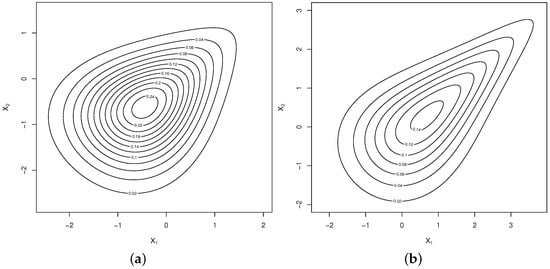
Figure 1. Contour plots: (a) BPHN(0,1,1.75,0,1,2.25,2), and (b) BPHN(0,1,0.5,0,1,0.75,0.75).

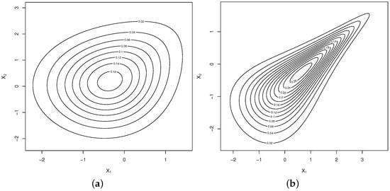
Figure 2. Contour plots: (a) BPHN(0,1,1.5,0,1,0.75,3.5), and (b) BPHN(0,1,0.75,0,1,2,0.5).

4.2. Parameter Estimation

In what follows, we consider the issue of estimating the parameters of the BPHN distribution. Given the dependency structure induced by Pareto copula, we use the maximum likelihood (ML) method, and the two-stage method (see [15]) to estimate the parameter vector $\mathit{\theta }={({\mu }_1,{\sigma }_1,{\alpha }_1,{\mu }_2,{\sigma }_2,{\alpha }_2,\alpha )}^{\prime }$. Initially, as in [5], we perform the following reparameterizations: ${\alpha }_1=\alpha {\gamma }_1$, and ${\alpha }_2=\alpha {\gamma }_2$, so that the interest is focused on the parameter vector ${\mathit{\theta }}_1={({\mu }_1,{\sigma }_1,{\gamma }_1,{\mu }_2,{\sigma }_2,{\gamma }_2,\alpha )}^{\prime }$. Thus, for a sample of size n from the $\mathrm{BPHN}({\mu }_1,{\sigma }_1,{\gamma }_1,{\mu }_2,{\sigma }_2,{\gamma }_2,\alpha )$ distribution, say $(x_{11},x_{12}),\dots ,(x_{n1},x_{n2})$, the log-likelihood function is given by

$$\begin{array}{cc}\hfill \ell \left({\mathit{\theta }}_1\right)& =n\left[log(\alpha +1)+log\left(\alpha \right)+\sum _{j=1}^{2}log\left({\gamma }_j\right)-\sum _{j=1}^{2}log\left({\sigma }_j\right)\right]\hfill \\ \hfill & +\sum _{i=1}^{n}log\left(\varphi \left(z_{i1}\right)\right)+\sum _{i=1}^{n}log\left(\varphi \left(z_{i2}\right)\right)\hfill \\ \hfill & -{\gamma }_1\sum _{i=1}^{n}log[1-\mathsf{\Phi }\left(z_{i1}\right)]-{\gamma }_2\sum _{i=1}^{n}log[1-\mathsf{\Phi }\left(z_{i2}\right)]\hfill \\ \hfill & -(\alpha +2)\sum _{i=1}^{n}log[{(1-\mathsf{\Phi }\left(z_{i1}\right))}^{-{\gamma }_1}+{(1-\mathsf{\Phi }\left(z_{i2}\right))}^{-{\gamma }_2}-1],\hfill \end{array}$$

where

$$z_{ij}=\frac{x_{ij}-{\mu }_j}{{\sigma }_j},j=1,2,i=1,2,\dots ,n.$$

The ML estimate ${\widehat{\mathit{\theta }}}_1={({\widehat{\mu }}_1,{\widehat{\sigma }}_1,{\widehat{\gamma }}_1,{\widehat{\mu }}_2,{\widehat{\sigma }}_2,{\widehat{\gamma }}_2,\widehat{\alpha })}^{\prime }$ of ${\mathit{\theta }}_1={({\mu }_1,{\sigma }_1,{\gamma }_1,{\mu }_2,{\sigma }_2,{\gamma }_2,\alpha )}^{\prime }$ can be obtained from the direct maximization of the log-likelihood function $\ell \left({\mathit{\theta }}_1\right)$ with respect to the model parameters. Using the R programming language, specifically applying the optim function, the maximization of the log-likelihood function can be performed. Also, using the invariance property of the ML estimator, we can easily obtain the ML estimates ${\widehat{\alpha }}_1$ and ${\widehat{\alpha }}_2$ of ${\alpha }_1$ and ${\alpha }_2$, respectively.

The score functions are

$$\begin{array}{cc}\hfill \frac{\partial \ell \left({\mathit{\theta }}_1\right)}{\partial {\mu }_j}& =\frac{1}{{\sigma }_j}\sum _{i=1}^n{z}_{ij}-\frac{{\gamma }_j}{{\sigma }_j}\sum _{i=1}^n\frac{\varphi \left(z_{ij}\right)}{1-\mathsf{\Phi }\left(z_{ij}\right)}\hfill \\ \hfill & +\frac{(\alpha +2){\gamma }_j}{{\sigma }_j}\sum _{i=1}^n\frac{\varphi \left(z_{ij}\right){(1-\mathsf{\Phi }\left(z_{ij}\right))}^{-{\gamma }_j-1}}{{(1-\mathsf{\Phi }\left(z_{i1}\right))}^{-{\gamma }_1}+{(1-\mathsf{\Phi }\left(z_{i2}\right))}^{-{\gamma }_2}-1},\hfill \end{array}$$

$$\begin{array}{cc}\hfill \frac{\partial \ell \left({\mathit{\theta }}_1\right)}{\partial {\sigma }_j}& =-\frac{n}{{\sigma }_j}+\frac{1}{{\sigma }_j}\sum _{i=1}^n{z}_{ij}^2-\frac{{\gamma }_j}{{\sigma }_j}\sum _{i=1}^n\frac{z_{ij}\varphi \left(z_{ij}\right)}{1-\mathsf{\Phi }\left(z_{ij}\right)}\hfill \\ \hfill & +\frac{(\alpha +2){\gamma }_j}{{\sigma }_j}\sum _{i=1}^n\frac{z_{ij}\varphi \left(z_{ij}\right){(1-\mathsf{\Phi }\left(z_{ij}\right))}^{-{\gamma }_j-1}}{{(1-\mathsf{\Phi }\left(z_{i1}\right))}^{-{\gamma }_1}+{(1-\mathsf{\Phi }\left(z_{i2}\right))}^{-{\gamma }_2}-1},\hfill \end{array}$$

$$\begin{array}{cc}\hfill \frac{\partial \ell \left({\mathit{\theta }}_1\right)}{\partial {\gamma }_j}& =\frac{n}{{\gamma }_j}-\sum _{i=1}^{n}log(1-\mathsf{\Phi }\left(z_{ij}\right))\hfill \\ \hfill & +(\alpha +2)\sum _{i=1}^n\frac{{(1-\mathsf{\Phi }\left(z_{ij}\right))}^{-{\gamma }_j}log(1-\mathsf{\Phi }\left(z_{ij}\right))}{{(1-\mathsf{\Phi }\left(z_{i1}\right))}^{-{\gamma }_1}+{(1-\mathsf{\Phi }\left(z_{i2}\right))}^{-{\gamma }_2}-1},\hfill \end{array}$$

$$\frac{\partial \ell \left({\mathit{\theta }}_1\right)}{\partial \alpha }=\frac{n}{\alpha +1}+\frac{n}{\alpha }-\sum _{i=1}^{n}log[{(1-\mathsf{\Phi }\left(z_{i1}\right))}^{-{\gamma }_1}+{(1-\mathsf{\Phi }\left(z_{i2}\right))}^{-{\gamma }_2}-1],$$

where $j=1,2$. The ML estimate ${\widehat{\mathit{\theta }}}_1={({\widehat{\mu }}_1,{\widehat{\sigma }}_1,{\widehat{\gamma }}_1,{\widehat{\mu }}_2,{\widehat{\sigma }}_2,{\widehat{\gamma }}_2,\widehat{\alpha })}^{\prime }$ can also be obtained by solving simultaneously the nonlinear system of equations

$$\left\{\begin{array}{c}{\displaystyle \frac{\partial \ell \left({\mathit{\theta }}_1\right)}{\partial {\mu }_j}=0,}\hfill \\ {\displaystyle \frac{\partial \ell \left({\mathit{\theta }}_1\right)}{\partial {\sigma }_j}=0,}\hfill \\ {\displaystyle \frac{\partial \ell \left({\mathit{\theta }}_1\right)}{\partial {\gamma }_j}=0,}\hfill \\ {\displaystyle \frac{\partial \ell \left({\mathit{\theta }}_1\right)}{\partial \alpha }=0.}\hfill \end{array}\right.$$

Numerical approaches are required for solving the above nonlinear system of equations, which requires the specification of initial values. To obtain initial values for the model parameters to be used in the iterative process, we can use the two-stage estimation procedure proposed by [15], since this procedure was defined for multivariate copula-based models. The first stage considers ML estimation from univariate marginals, while the second stage considers ML estimation of the dependence parameter with the other parameters held fixed from the first stage:

• First stage. Considering that $X_j\sim \mathrm{PHN}({\mu }_j,{\sigma }_j,{\alpha }_j)$ for $j=1,2$. We have that the ML estimaties of ${\mu }_j$, ${\sigma }_j$ and ${\alpha }_j$ are obtained from the solutions of the nonlinear equations

  $$\left\{\begin{array}{c}{\displaystyle \frac{n}{{\alpha }_j}+\sum _{i=1}^{n}log(1-\mathsf{\Phi }\left(z_{ij}\right))=0,}\hfill \\ {\displaystyle \sum _{i=1}^n{z}_{ij}+({\alpha }_j-1)\sum _{i=1}^n{W}_{ij}=0,}\hfill \\ {\displaystyle \sum _{i=1}^n{z}_{ij}^2+(\alpha +1)\sum _{i=1}^n{z}_{ij}{W}_{ij}=n,}\hfill \end{array}\right.$$

  where

  $$W_{ij}=\frac{\varphi \left(z_{ij}\right)}{1-\mathsf{\Phi }\left(z_{ij}\right)},j=1,2,i=1,2,\dots ,n.$$

  The solution of the previous system of equations for each j allows us to obtain the ML estimates ${\tilde{\mu }}_j,$ ${\tilde{\sigma }}_j$ and ${\tilde{\alpha }}_j$ of ${\mu }_j$, ${\sigma }_j$ and ${\alpha }_j$, respectively, for $j=1,2$.
• Second stage. In this stage, we estimate the parameter $\alpha$ by replacing the unknown parameters with the ML estimates from the previous stage and then maximize the resulting log-likelihood function; that is, we need to maximize the function

  $$L\left(\alpha \right)=\sum _{i=1}log[C_{\alpha }({(1-\mathsf{\Phi }\left(z_{i1}\right))}^{-{\widehat{\alpha }}_1},{(1-\mathsf{\Phi }\left(z_{i2}\right))}^{-{\widehat{\alpha }}_2}],$$

  where

  $$\begin{array}{cc}\hfill log\left[C_{\alpha }(u,v)\right]& =log\left(\frac{\alpha +1}{\alpha }\right)-\left(1+\frac{1}{\alpha }\right)log\left((1-u)(1-v)\right)\hfill \\ \hfill & -(\alpha +2)log[{(1-u)}^{-\frac{1}{\alpha }}+{(1-v)}^{-\frac{1}{\alpha }}-1],\hfill \end{array}$$

  so that we have the score function

  $$\begin{array}{cc}\hfill \frac{\partial L\left(\alpha \right)}{\partial \alpha }& =-\frac{1}{\alpha (\alpha +1)}+\frac{1}{{\alpha }^2}log\left[(1-u)(1-v)\right]\hfill \\ \hfill & -log[{(1-u)}^{-\frac{1}{\alpha }}+{(1-v)}^{-\frac{1}{\alpha }}-1].\hfill \end{array}$$

  The solution of the resulting equation $\partial L\left(\alpha \right)/\partial \alpha =0$ lead us to the estimate $\tilde{\alpha }$ of $\alpha$.

We can also consider another alternative to obtain initial values for the model parameters by using the method proposed by [16], where we initially normalize each variable to obtain a model that depends only on ${\alpha }_1$, ${\alpha }_2$ and $\alpha$; that is, we have the log-likelihood function

$$\begin{array}{cc}\hfill \ell ({\gamma }_1,{\gamma }_2,\alpha )& =\alpha nlog\left(\alpha (\alpha +1){\gamma }_1{\gamma }_2\right)-\sum _{i=1}^n\sum _{j=1}^2{\gamma }_{j}log(1-\mathsf{\Phi }\left(z_{ij}\right))\hfill \\ \hfill & -(\alpha +2)\sum _{i=1}^{n}log({(1-\mathsf{\Phi }\left(z_{i1}\right))}^{-{\gamma }_1}+{(1-\mathsf{\Phi }\left(z_{i2}\right))}^{-{\gamma }_2}-1).\hfill \end{array}$$

After doing

$$\frac{\partial \ell ({\gamma }_1,{\gamma }_2,\alpha )}{\partial \alpha }=0,$$

we obtain

$$\tilde{\alpha }({\gamma }_1,{\gamma }_2)=\frac{(2-A)+\sqrt{4+A^2}}{2A},$$

where

$$A:=A({\gamma }_1,{\gamma }_2)=\frac{1}{n}\sum _{i=1}^{n}log({(1-\mathsf{\Phi }\left(z_{i1}\right))}^{-{\gamma }_1}+{(1-\mathsf{\Phi }\left(z_{i2}\right))}^{-{\gamma }_2}-1).$$

Thus, the new profiled log-likelihood function ${\ell }_p(\tilde{\alpha }({\gamma }_1,{\gamma }_2),{\gamma }_1,{\gamma }_2)$ is reached. After obtaining the estimates ${\tilde{\gamma }}_1$ and ${\tilde{\gamma }}_2$ of ${\gamma }_1$ and ${\gamma }_2$, respectively, we then obtain an estimate for $\alpha$ as $\tilde{\alpha }({\tilde{\gamma }}_1,{\tilde{\gamma }}_2)$. We can take as initial values for ${\mu }_1$ and ${\mu }_2$ the sample means, and for ${\sigma }_1$ and ${\sigma }_2$ the sample standard deviations, or we can replace ${\tilde{\gamma }}_1$, $\widetilde{{\gamma }_2}$ and $\tilde{\alpha }$ in the original log-likelihood to obtain the initial values for ${\mu }_1$, ${\mu }_2$, ${\sigma }_1$ and ${\sigma }_2$.

When n is large, we have that ${\widehat{\mathit{\theta }}}_1\stackrel{a}{\sim }{\mathcal{N}}_7({\mathit{\theta }}_1,\mathit{J}{\left({\mathit{\theta }}_1\right)}^{-1})$, where “$\stackrel{a}{\sim }$” means approximately distributed, $\mathit{J}\left({\mathit{\theta }}_1\right)=-E\left(\mathit{H}\left({\mathit{\theta }}_1\right)\right)$ is the expected Fisher information matrix for ${\mathit{\theta }}_1$, and $\mathit{H}\left({\mathit{\theta }}_1\right)={\partial }^2\ell \left({\mathit{\theta }}_1\right)/\partial {\mathit{\theta }}_1\partial {\mathit{\theta }}_1^{\prime }$ is the Hessian matrix, whose elements are provided in the Appendix A. Using the transformation method, we have that $\widehat{\mathit{\theta }}\stackrel{a}{\sim }{\mathcal{N}}_7(\mathit{\theta },\mathit{K}{\left(\mathit{\theta }\right)}^{-1})$, where $\mathit{K}\left(\mathit{\theta }\right)={\mathit{D}}^{\prime }\mathit{J}\left({\mathit{\theta }}_1\right)\mathit{D}$ with $\mathit{K}{\left(\mathit{\theta }\right)}^{-1}$ denoting its inverse, and

$$\mathit{D}=\left(\begin{array}{ccccccc}1& 0& 0& 0& 0& 0& 0\\ 0& 1& 0& 0& 0& 0& 0\\ 0& 0& \alpha & 0& 0& 0& {\displaystyle \frac{{\alpha }_1}{\alpha }}\\ 0& 0& 0& 1& 0& 0& 0\\ 0& 0& 0& 0& 1& 0& 0\\ 0& 0& 0& 0& 0& \alpha & {\displaystyle \frac{{\alpha }_2}{\alpha }}\\ 0& 0& -{\displaystyle \frac{\alpha }{{\alpha }_1}}& 0& 0& -{\displaystyle \frac{\alpha }{{\alpha }_2}}& 1\end{array}\right).$$

The elements of $\mathit{J}\left({\mathit{\theta }}_1\right)$ are obtained in terms of numerical integration. On the other hand, the observed Fisher information matrix given by $-\mathit{H}\left({\widehat{\mathit{\theta }}}_1\right)$ can also be used for computing asymptotic standard errors for the ML estimates of the model parameters (see Appendix A). After computing $-\mathit{H}\left({\widehat{\mathit{\theta }}}_1\right)$, we obtain the observed Fisher information matrix under $\mathit{\theta }$-parametrization as $-{\widehat{\mathit{D}}}^{\prime }\mathit{H}\left({\widehat{\mathit{\theta }}}_1\right)\widehat{\mathit{D}}$, where $\widehat{\mathit{D}}:=\mathit{D}({\widehat{\alpha }}_1,{\widehat{\alpha }}_2,\widehat{\alpha })$. It is worth emphisizing that the observed information matrix can be computed numerically from standard maximization routines, which now provide the observed information matrix as part of their output. For example, one can use the R functions optim or nlm to compute the observed Fisher information matrix numerically.

4.3. Monte Carlo Simulation

In the following, we consider Monte Carlo simulation experiments to evaluate the performance of the ML estimation procedure discussed in the previous section to estimate the BPHN distribution parameters. It is worth emphasizing that is rather easy to generate random variates from the BPHN distribution. We consider the following steps to generate $(X_1,X_2)$ from $\mathrm{BPHN}({\mu }_1,{\sigma }_1,{\alpha }_1,{\mu }_2,{\sigma }_2,{\alpha }_2,\alpha )$ distribution:

Step 1.

Generate two independent random variates $U_1\sim \mathcal{U}(0,1)$ and $U_2\sim \mathcal{U}(0,1)$, where $\mathcal{U}(0,1)$ means a uniform distribution on $(0,1)$.

Step 2.

Compute

$$X_2={\mu }_2+{\sigma }_2{\mathsf{\Phi }}^{-1}(1-{(1-U_2)}^{1/{\alpha }_2}),$$

where ${\mathsf{\Phi }}^{-1}(·)$ is the standard normal quantile function.

Step 3.

Define $B_1={[1-\mathsf{\Phi }\left(X_2\right)]}^{-{\alpha }_2(\alpha +1)/\alpha }$ and $B_2={[1-\mathsf{\Phi }\left(X_2\right)]}^{-{\alpha }_2/\alpha }-1$. Let $B_3={[{(B_1/U_1)}^{1/(\alpha +1)}-B_2]}^{-\alpha /{\alpha }_1}$. For each value of $X_2$, compute

$$X_1={\mu }_1+{\sigma }_1{\mathsf{\Phi }}^{-1}(1-B_3).$$

Then, $(X_1,X_2)\sim \mathrm{BPHN}({\mu }_1,{\sigma }_1,{\alpha }_1,{\mu }_2,{\sigma }_2,{\alpha }_2,\alpha )$.

The Monte Carlo experiments were performed using the R programming language, and we consider 10,000 Monte Carlo replications. The performance of the ML procedure to estimate the BPHN distribution parameters was evaluated on the basis of the following quantities for each sample size: the empirical mean, and the empirical standard deviation, which are computed from 10,000 replications. The sample sizes we consider are $n=90$ and 150. Without loss of generality, we consider ${\mu }_1=1.5$, ${\sigma }_1={\sigma }_2=1.0$, ${\alpha }_1=0.5$, ${\mu }_2=-0.5$, ${\alpha }_2=1.2$, and $\alpha =0.2$, $0.4$, $0.6$, $0.8$, $1.0$, $1.2$ and $1.5$. The emprical mean is listed in Table 1, while the empirical standard deviation is listed in Table 2. In general, from Table 1, note that the ML estimates of ${\mu }_1$, ${\sigma }_1$, ${\alpha }_1$, ${\mu }_2$, ${\sigma }_2$ and ${\alpha }_2$ are close to their respective true values, while the parameter that controls the dependence in the Pareto copula, $\alpha$, is overestimated, mainly as this parameter increases. As expected, the standard deviation of the ML estimates of all parameters decreases as the sample size increases (see Table 2). In short, the Monte Carlo simulation experiments reveal that the ML method can be used effectively to estimate the BPHN parameters.

Table 1. Parameter estimates; empirical mean.

n	$\mathit{\alpha }$	${\mathit{\mu }}_{\mathbf{1}}$	${\mathit{\sigma }}_{\mathbf{1}}$	${\mathit{\alpha }}_{\mathbf{1}}$	${\mathit{\mu }}_{\mathbf{2}}$	${\mathit{\sigma }}_{\mathbf{2}}$	${\mathit{\alpha }}_{\mathbf{2}}$	$\mathit{\alpha }$
90	0.2	1.024	0.876	0.495	−0.378	1.034	1.539	0.321
	0.4	1.192	0.903	0.566	−0.403	1.008	1.371	0.632
	0.6	1.364	0.950	0.665	−0.483	0.986	1.271	0.941
	0.8	1.376	0.948	0.632	−0.555	0.965	1.176	1.256
	0.8	1.419	0.959	0.651	−0.576	0.959	1.178	1.553
	1.0	1.406	0.953	0.619	−0.591	0.956	1.145	1.821
	1.5	1.426	0.962	0.613	−0.612	0.949	1.121	2.303
150	0.2	0.990	0.864	0.471	−0.339	1.053	1.599	0.318
	0.4	1.172	0.898	0.540	−0.395	1.016	1.362	0.625
	0.6	1.319	0.936	0.608	−0.487	0.991	1.248	0.931
	0.8	1.391	0.955	0.635	−0.550	0.974	1.167	1.224
	1.0	1.427	0.963	0.643	−0.543	0.978	1.182	1.523
	1.2	1.430	0.963	0.628	−0.552	0.976	1.178	1.805
	1.5	1.458	0.972	0.627	−0.601	0.960	1.125	2.192

Table 2. Parameter estimates; empirical standard deviation.

n	$\mathit{\alpha }$	${\mathit{\mu }}_{\mathbf{1}}$	${\mathit{\sigma }}_{\mathbf{1}}$	${\mathit{\alpha }}_{\mathbf{1}}$	${\mathit{\mu }}_{\mathbf{2}}$	${\mathit{\sigma }}_{\mathbf{2}}$	${\mathit{\alpha }}_{\mathbf{2}}$	$\mathit{\alpha }$
90	0.2	0.251	0.117	0.158	0.195	0.081	0.326	0.037
	0.4	0.370	0.152	0.259	0.273	0.102	0.416	0.089
	0.6	0.460	0.175	0.389	0.314	0.117	0.452	0.153
	0.8	0.426	0.169	0.319	0.315	0.117	0.412	0.248
	1.0	0.480	0.178	0.372	0.387	0.137	0.533	0.348
	1.2	0.470	0.180	0.329	0.368	0.135	0.465	0.387
	1.5	0.463	0.181	0.326	0.364	0.124	0.483	0.620
150	0.2	0.236	0.103	0.147	0.193	0.072	0.326	0.028
	0.4	0.289	0.120	0.202	0.207	0.075	0.312	0.065
	0.6	0.348	0.137	0.255	0.263	0.094	0.359	0.113
	0.8	0.384	0.149	0.295	0.283	0.100	0.359	0.165
	1.0	0.420	0.156	0.317	0.293	0.101	0.378	0.223
	1.2	0.431	0.164	0.311	0.316	0.109	0.411	0.290
	1.5	0.432	0.161	0.311	0.352	0.119	0.428	0.368

5. Real Data Application

Next, we consider an application of the BPHN distribution to real data for illustrative purposes. The data set contains two different measures of stiffness of each of the 30 boards. The considered stiffness measures are the Shock ($X_1$) and Vibration ($X_2$) of each of the 30 boards. The data were reported by [17]. The first measurement involves sending a shock wave down the board, and the second measurement is determined while vibrating the board. All numerical computations provided in this were done by using the R program.

We assume that $(X_{1i},X_{2i})\sim \mathrm{BPHN}({\mu }_1,{\sigma }_1,{\alpha }_1,{\mu }_2,{\sigma }_2,{\alpha }_2,\alpha )$ for $i=1,2,\dots ,30$. To estimate the BPHN model parameters, we initially estimate the marginal PDFs corresponding to each variable. We thus obtain the following estimates: ${\tilde{\mu }}_1=1554.82$, ${\tilde{\sigma }}_1=176.34$, ${\tilde{\alpha }}_1=0.18$, ${\tilde{\mu }}_2=1393.59$, ${\tilde{\sigma }}_2=173.79$, and ${\tilde{\alpha }}_2=0.17$. Figure 3a,b display the QQ-plots for the estimated marginal distributions. Note the goodness-of-fit of each estimated marginal distribution to the real data, which means that the BPHN distribution may be a good choice for modeling these data. Now, using the above estimates in the copula function, we obtain an estimate for the parameter $\alpha$, that is, $\tilde{\alpha }=0.35$. Finally, taking the above estimates as initial values for the iterative process, we obtain the following ML estimates (standard errors in parentheses): ${\widehat{\mu }}_1=1529.91\left(184.47\right)$, ${\widehat{\sigma }}_1=277.53\left(48.13\right)$, ${\widehat{\alpha }}_1=0.28\left(0.17\right)$, ${\widehat{\mu }}_2=1428.44\left(87.82\right)$, ${\widehat{\sigma }}_2=184.49\left(33.33\right)$, ${\widehat{\alpha }}_2=0.16\left(0.05\right)$, and $\widehat{\alpha }=0.27\left(0.12\right)$. Visual inspection of the contour plot in Figure 3c confirms a satisfactory fit of the BPHN distribution to the data.

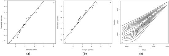
Figure 3. QQ-plots and contour plot: (a) Shock, (b) Vibration, and (c) contour plot of the BPHN distribution.

Next, for the sake of comparison, we also consider the following bivariate distributions to fit the current real data: the bivariate skew-normal conditional (BVSNC) distribution introduced by [9], denoted by BVSNC$({\xi }_1,{\eta }_1,{\xi }_2,{\eta }_2,\lambda )$, and the bivariate Birnbaum-Saunders (BVBS) distribution studied by [10], denoted by BVBS$({\alpha }_1,{\beta }_1,{\alpha }_2,{\beta }_2,\lambda )$. The ML estimates (standard errors in parentheses) of the BVSNC parameters are ${\widehat{\xi }}_1=1927.51\left(26.65\right),$ ${\widehat{\xi }}_2=1745.35\left(30.38\right),$ ${\widehat{\eta }}_1=320.31\left(41.40\right),$ ${\widehat{\eta }}_2=313.23\left(40.43\right)$ and $\widehat{\lambda }=10.88\left(5.01\right)$, whereas the ML estimates (standard errors in parentheses) of the BVBS parameters are ${\widehat{\alpha }}_1=0.1621\left(0.0210\right),$ ${\widehat{\alpha }}_2=0.1701\left(0.0219\right),$ ${\widehat{\beta }}_1=1917.22\left(22.26\right),$ ${\widehat{\beta }}_2=1734.76\left(29.32\right)$ and $\widehat{\lambda }=10.29\left(4.86\right)$. To compare the bivariate distributions, we make use of the Akaike information criterion (AIC), and Bayesian information criterion (BIC). The smaller the values of AIC and BIC, the better the fitted distribution to the real data. Table 3 lists the AIC and BIC values for all bivariate distributions, which leads to the conclusion that the BPHN distribution is better than the other bivariate distributions to model the current bivariate real data.

Table 3. AIC and BIC values.

Measure	BVSNC	BVBS	BPHN
AIC	842.99	835.82	828.27
BIC	850.00	842.83	838.08

6. Concluding Remarks

The univariate proportional hazard distribution has found several applications in the literature and has many attractive properties. However, the extension of the univariate proportional hazard distribution in a multivariate setting has been so neglected in the statistical literature. In this paper, based on the Pareto copula, we have introduced a simple and tractable bivariate proportional hazard family of distributions that may be very useful to deal with bivariate data in practice. We also derive several distribution properties for this bivariate family of distributions. In addition, we particularize this general bivariate distribution to the case where the univariate normal distribution is considered, so that the bivariate proportional hazard normal distribution is obtained. The estimation of the bivariate proportional hazard normal model parameters is approached by the maximum likelihood method, and the observed and expected Fisher information matrixes are derived. Finally, an application to real data set is presented to illustrate the bivariate proportional hazard normal distribution in practice.

References

- Durrans, S.R. Distributions of fractional order statistics in hydrology. Water Resour. Res. 1992, 28, 1649–1655. [Google Scholar] [CrossRef]
- Martínez-Flórez, G.; Moreno-Arenas, G.; Vergara-Cardoso, S. Properties and Inference for Proportional Hazard Models. Colomb. J. Stat. 2013, 36, 95–114. [Google Scholar]
- Wang, B.; Yu, K.; Jones, M. Inference under progressively type II right-censored sampling for certain lifetime distributions. Technometrics 2010, 52, 453–460. [Google Scholar] [CrossRef]
- Cordeiro, G.M.; de Castro, M. A new family of generalized distributions. J. Stat. Comput. Simul. 2011, 81, 883–898. [Google Scholar] [CrossRef]
- Kundu, D.; Gupta, R. Power normal distribution. Statistics 2013, 47, 110–125. [Google Scholar] [CrossRef]
- Clayton, D.G. A model for association in bivariate life tables and its application in epidemiological studies of familial tendency in chronic disease incidence. Biometrika 1978, 65, 141–152. [Google Scholar] [CrossRef]
- Kimeldorf, G.; Sampson, A.R. Uniform representations of bivariate distributions. Commun. Stat. Theory Methods 1975, 4, 617–627. [Google Scholar] [CrossRef]
- Cook, R.D.; Johnson, M.E. A family of distributions for modelling non-elliptically symmetric multivariate data. J. R. Stat. Soc. B 1981, 43, 210–218. [Google Scholar] [CrossRef]
- Arnold, B.C.; Castilho, E.; Sarabia, J.M. Conditionally specified multivariate skewed distributions. Sankhya A 2002, 64, 206–226. [Google Scholar]
- Lemonte, A.J.; Martínez-Flórez, G.; Moreno-Arenas, G. Multivariate Birnbaum–Saunders distribution: Properties and associated inference. J. Stat. Comput. Simul. 2015, 85, 374–392. [Google Scholar] [CrossRef]
- Martínez-Flórez, G.; Lemonte, A.J.; Salinas, H.S. Multivariate skew-power-normal distributions: Properties and associated inference. Symmetry 2019, 11, 1509. [Google Scholar] [CrossRef]
- Zhang, L.; Xu, A.; An, L.; Li, M. Bayesian inference of system reliability for multicomponent stress-strength model under Marshall-Olkin Weibull distribution. Systems 2022, 10, 196. [Google Scholar] [CrossRef]
- Nelsen, R.B. An Introduction to Copulas; Springer: New York, NY, USA, 2006. [Google Scholar]
- Marshall, A.W. Some comments on the hazard gradient. Stoch. Process. Their Appl. 1975, 3, 293–300. [Google Scholar] [CrossRef]
- Joe, H. Asymptotic efficiency of two-stage estimation method for copula-based models. J. Multivar. Anal. 2005, 94, 401–419. [Google Scholar] [CrossRef]
- Gupta, D.; Gupta, R.C. Analyzing skewed data by power normal model. Test 2008, 17, 197–210. [Google Scholar] [CrossRef]
- Johnson, R.A.; Wichern, D.W. Applied Multivariate Statistical Analysis; Pearson Prentice Hall: Upper Saddle River, NJ, USA, 2007. [Google Scholar]
Publisher’s Note: MDPI stays neutral with regard to jurisdictional claims in published maps and institutional affiliations. |
© 2022 by the authors. Licensee MDPI, Basel, Switzerland. This article is an open access article distributed under the terms and conditions of the Creative Commons Attribution (CC BY) license (https://creativecommons.org/licenses/by/4.0/).