Ergodicity Bounds and Limiting Characteristics for a Modified Prendiville Model

Abstract

We consider the time-inhomogeneous Prendiville model with failures and repairs. The property of weak ergodicity is considered, and estimates of the rate of convergence for the main probabilistic characteristics of the model are obtained. Several examples are considered showing how such estimates are obtained and how the limiting characteristics themselves are constructed.

1. Introduction

Nonstationary queuing systems are of constant interest, since these models adequately describe the actual behavior of many real processes in various applied fields.

Inhomogeneous Markov chains with finite state space are widely applied in queuing systems, for example, in biology, computer science, high-load information systems, etc. (see [1,2,3]). Queuing theory remains an actively developing branch of applied probability theory. Continuous-time Markov chains have proven to be good tools for stochastic modeling in the natural and technical sciences, such as telecommunication, biology, chemistry, etc. In the study of such models an important role is assigned to the evaluation of their meaningful probabilistic characteristics. In some cases, the study of the probabilistic characteristics of queuing systems can be reduced to the study of the forward Kolmogorov system.

The first estimates of the convergence rate of the characteristics of nonstationary queuing systems to the limit mode were obtained by Gnedenko, for details, see [4].

The logistic model was proposed in 1949 by Prendiville [5] and was subsequently solved in 1956 by Takashima [6]. This model was later applied in biology, ecology, and queuing systems (see, e.g., [1,5,6,7]). The Prendiville process can be also viewed as the continuous-time Ehrenfest model (see [8,9]). Zheng [10] extended the Prendiville process to the inhomogeneous case. The inhomogeneous situation was studied in [11]. The rate of convergence and stability of this model was firstly studied by Mitrophanov in [12]. The Prendiville model in the presence of jumps has been studied in [13]. Note that the usual Prendiville model is a special case of the birth–death process. This means that it can be studied in detail in the way described in our previous papers, see [2].

Recently, much attention has been paid to the study of queuing systems with disasters and repairs. The concept of disasters occurring at a random time leading to the complete departure of all the requirements existing at that time and the instantaneous inactivation of the service object until a new arrival of the requirement, can be often found in many practical situations. Such models, for example, were studied in [14].

In [15], the Prendiville growth mechanism, which assumes a linearly decreasing population growth rate, was generalized to a multi-compartment system by Parthasarathy and Kumar [16]. A diagnostic test was presented to indicate the parameter vectors for which this first approximation was not very accurate.

In [14], a time-inhomogeneous birth–death process with a finite state space was considered under the assumption that failures and repairs can occur at random time instants. Specifically, the state space of the considered stochastic process, in addition to the operating states, included two particular states, denoted by F and R. The dynamic system started from any state j (operating, F, R). Due to a failure that occurred according to a nonstationary exponential distribution, a transition from an operating state to F occurred, after which a repair, that led to the state R, starting from F, was required. The repair times were assumed to be random and follow a nonstationary exponential distribution. After the system was repaired, it restarted from one of the operating states.

The contributions of this paper can be summarized as follows:

• In the first approach, we examine the standard way to eliminate the state with the minimum number and then apply the diagonal transformation. Previously, this type of transformation (using a triangular matrix) was considered in [17]. This approach allows one to obtain exhaustive estimates of the rate of convergence to the limiting mode in the space $l_1$.
• Using the second approach, we pass from the forward Kolmogorov system to a system of the form $\frac{d\mathbf{z}}{dt}=W\left(t\right)\mathbf{z}\left(t\right)$ for $t\ge 0,$ (see [18]). This method was previously applied to the study of one class of supercomputer systems in [3] (for nonstationary models, simple methods for solving the forward Kolmogorov system do not give good results).
• We also briefly review some issues related to proportional intensities and perturbation bounds.
• Numerical examples are considered, in which estimates of the rate of convergence to the limit mode are obtained and the limit characteristics themselves are constructed.

2. Model Description and Basic Notions

A detailed description of the process was presented in [14], we will briefly explain it here.

Let $X\left(t\right),t\ge 0$ be a continuous-time (in general, inhomogeneous) Markov chain on the finite state space $\{-2,-1,0,1,2,\dots ,N\}$, where ’$-2$’ corresponds to the failure state F, ’$-1$’ corresponds to the repair state R, and other indexes correspond to the operating states of the queue.

We denote the transition probabilities by $p_{ij}(s,t)=P\{X\left(t\right)=j|X\left(s\right)=i\}$, the state probabilities by $p_i\left(t\right)=P\{X\left(t\right)=i\}$; and we let $\mathbf{p}\left(t\right)={(p_{-2}\left(t\right),p_{-1}\left(t\right),p_0\left(t\right),p_1\left(t\right),\dots ,p_N\left(t\right))}^T$ be the corresponding probability distribution vector for $X\left(t\right)$ at time t.

We suppose that possible transitions of $X\left(t\right)$ are as follows:

• $k\to k+1$ with intensity function ${\lambda }_k\left(t\right)$ for $k=0,1,\dots ,N-1$,
• $k\to k-1$ with intensity function ${\mu }_k\left(t\right)$ for $k=1,2,\dots ,N$,
• $-1\to k$ with intensity function ${\gamma }_k\left(t\right)$ for $k=0,1,\dots ,N$,
• $k\to -2$ with intensity function ${\zeta }_k\left(t\right)$ for $k=0,1,\dots ,N$,
• $-2\to -1$ with intensity function $Q\left(t\right)$.

We assume that all intensity functions are nonnegative and locally integrable on the interval $[0,\infty )$.

The corresponding graph of possible transitions is shown in Figure 1.

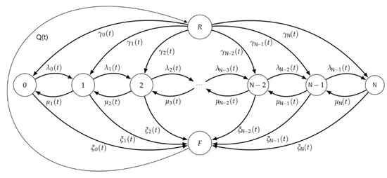
Figure 1. State graph.

Set $a_{ij}\left(t\right)=q_{ji}\left(t\right)$ for $i\ne j$ and $a_{ii}\left(t\right)=-{\sum }_{i\ne j}{a}_{ji}\left(t\right)=-{\sum }_{i\ne j}{q}_{ij}\left(t\right)$.

Then, the transposed intensity matrix $A\left(t\right)=Q^T\left(t\right)$ has the form

$$A\left(t\right)=\left(\begin{array}{cccccc}-Q\left(t\right)& 0& {\zeta }_0\left(t\right)& {\zeta }_1\left(t\right)& \cdots & {\zeta }_N\left(t\right)\\ Q\left(t\right)& -\Omega \left(t\right)& 0& 0& \cdots & 0\\ 0& {\gamma }_0\left(t\right)& -({\lambda }_0\left(t\right)+{\zeta }_0\left(t\right))& {\mu }_1\left(t\right)& \cdots & 0\\ 0& {\gamma }_1\left(t\right)& {\lambda }_0\left(t\right)& -({\lambda }_1\left(t\right)+{\mu }_1\left(t\right)+{\zeta }_1\left(t\right))& \cdots & ⋮\\ 0& {\gamma }_2\left(t\right)& 0& {\lambda }_1\left(t\right)& \ddots & 0\\ ⋮& ⋮& ⋮& ⋮& \cdots & {\mu }_N\left(t\right)\\ 0& {\gamma }_N\left(t\right)& 0& \cdots & {\lambda }_{N-1}\left(t\right)& -({\mu }_N\left(t\right)+{\zeta }_N\left(t\right))\end{array}\right),$$

(1)

where $\Omega \left(t\right)={\sum }_{k=0}^N{\gamma }_k\left(t\right)$, and the forward Kolmogorov system for $X\left(t\right)$ has the form

$$\frac{d\mathbf{p}\left(t\right)}{dt}=A\left(t\right)\mathbf{p}\left(t\right).$$

(2)

We denote by $\parallel ·\parallel$ the $l_1$-norm, and $\parallel \mathbf{x}\parallel =\sum |x_i|$, $\parallel B\parallel ={max}_j{\sum }_i\left|b_{ij}\right|$ for matrix $B=\left(b_{ij}\right)$.

Recall that a Markov chain $X\left(t\right)$ is called weakly ergodic, if $\parallel {\mathbf{p}}^{*}\left(t\right)-{\mathbf{p}}^{**}\left(t\right)\parallel \to 0$ as $t\to \infty$ for any initial conditions ${\mathbf{p}}^{*}\left(0\right)$ and ${\mathbf{p}}^{**}\left(0\right)$, where ${\mathbf{p}}^{*}\left(t\right)$ and ${\mathbf{p}}^{**}\left(t\right)$ are the corresponding solutions of (2).

Both of our approaches are based on the logarithmic norm method; see our previous papers (for instance, the recent publications [2,19]) for details.

3. First Approach

The first approach is based on excluding the state with the minimum number, see for instance [2].

Excluding the ’$-2$’ state, one can rewrite (2) as

$$\frac{d\mathbf{z}\left(t\right)}{dt}=B\left(t\right)\mathbf{z}\left(t\right)+f\left(t\right),$$

(3)

where $\mathbf{z}\left(t\right)={(p_{-1}\left(t\right),p_0\left(t\right),p_1\left(t\right),\cdots ,p_N\left(t\right))}^T$, $f\left(t\right)=\left(Q\right(t),0,\cdots ,0)$.

$$\begin{array}{c}\hfill B\left(t\right)=\left(\begin{array}{ccccc}-(\Omega (t)+Q(t\left)\right)& -Q\left(t\right)& -Q\left(t\right)& \cdots & -Q\left(t\right)\\ {\gamma }_0\left(t\right)& -({\lambda }_0\left(t\right)+{\zeta }_0\left(t\right))& {\mu }_1\left(t\right)& \cdots & 0\\ {\gamma }_1\left(t\right)& {\lambda }_0\left(t\right)& -({\lambda }_1\left(t\right)+{\mu }_1\left(t\right)+{\zeta }_1\left(t\right))& \cdots & ⋮\\ {\gamma }_2\left(t\right)& 0& {\lambda }_1\left(t\right)& \ddots & 0\\ ⋮& ⋮& ⋮& \cdots & {\mu }_N\left(t\right)\\ {\gamma }_N\left(t\right)& 0& \cdots & {\lambda }_{N-1}\left(t\right)& -({\mu }_N\left(t\right)+{\zeta }_N\left(t\right))\end{array}\right).\end{array}$$

Theorem 1.

Let ${\zeta }_{*}\left(t\right)\ge Q\left(t\right)$ for almost all $t\ge 0$, and

$$\underset{0}{\overset{+\infty }{\int }}{\beta }_{*}\left(\tau \right)d\tau =+\infty .$$

(4)

Then the queue-length process $X\left(t\right)$ is weakly ergodic and the following bound holds:

$$\parallel {\mathbf{p}}^{*}\left(t\right)-{\mathbf{p}}^{**}\left(t\right)\parallel \le 2e^{-\underset{0}{\overset{t}{\int }}{\beta }_{*}\left(\tau \right)d\tau },$$

(5)

for any initial conditions ${\mathbf{p}}^{*}\left(0\right)$, ${\mathbf{p}}^{**}\left(0\right)$, and any $t\ge 0$.

Proof. 

Recall that with the account of the chosen norm, the logarithmic norm of a matrix function $B\left(t\right)=\left(b_{ij}\left(t\right)\right)$ is calculated by the formula

$$\gamma \left(B\left(t\right)\right)=\underset{j}{max}\left(b_{jj}\left(t\right)+\sum _{i\ne j}\left|b_{ij}\left(t\right)\right|\right).$$

Moreover, in all situations under consideration, the diagonal elements of the matrices are negative, which means that we can write

$$\gamma \left(B\left(t\right)\right)=-\underset{j}{min}{\alpha }_j\left(t\right),\mathrm{where}{\alpha }_j\left(t\right)=|b_{jj}\left(t\right)|-\sum _{i\ne j}\left|b_{ij}\left(t\right)\right|.$$

Denote ${\zeta }_{*}\left(t\right)={min}_{0\le j\le N}\left({\zeta }_j\left(t\right)\right)$, and suppose that ${\zeta }_{*}\left(t\right)\ge Q\left(t\right)$ for almost all $t\ge 0$. Then,

$$\gamma \left(B\left(t\right)\right)=-{\beta }_{*}\left(t\right)=-min(Q\left(t\right),{\zeta }_{*}\left(t\right)-Q\left(t\right)).$$

Hence, we obtain the estimate (5). □

This proposition can be slightly generalized.

Let $d_i$ be some positive numbers, D be the corresponding diagonal matrix:

$$D=\left(\begin{array}{ccccc}{d}_{-1}& 0& 0& \cdots & 0\\ 0& d_0& 0& \cdots & 0\\ 0& 0& d_1& \cdots & 0\\ 0& ⋮& ⋮& \ddots & ⋮\\ 0& 0& \cdots & \cdots & d_N\end{array}\right),$$

and ${\parallel \mathbf{z}\left(t\right)\parallel }_{1D}={\parallel D\mathbf{z}\left(t\right)\parallel }_1$.

Then, $DB\left(t\right)D^{-1}$ has the form

$$\left(\begin{array}{ccccc}-(\Omega (t)+Q(t\left)\right)& -Q\left(t\right)\frac{d_{-1}}{d_0}& -Q\left(t\right)\frac{d_{-1}}{d_1}& \cdots & -Q\left(t\right)\frac{d_{-1}}{d_N}\\ {\gamma }_0\left(t\right)\frac{d_0}{d_{-1}}& -({\lambda }_0\left(t\right)+{\zeta }_0\left(t\right))& {\mu }_1\left(t\right)\frac{d_0}{d_1}& \cdots & 0\\ {\gamma }_1\left(t\right)\frac{d_1}{d_{-1}}& {\lambda }_0\left(t\right)\frac{d_1}{d_0}& -({\lambda }_1\left(t\right)+{\mu }_1\left(t\right)+{\zeta }_1\left(t\right))& \cdots & ⋮\\ {\gamma }_2\left(t\right)\frac{d_2}{d_{-1}}& 0& {\lambda }_1\left(t\right)\frac{d_2}{d_1}& \ddots & 0\\ ⋮& ⋮& ⋮& \cdots & {\mu }_N\left(t\right)\frac{d_{N-1}}{d_N}\\ {\gamma }_N\left(t\right)\frac{d_N}{d_{-1}}& 0& \cdots & {\lambda }_{N-1}\left(t\right)\frac{d_N}{d_{N-1}}& -({\mu }_N\left(t\right)+{\zeta }_N\left(t\right))\end{array}\right),$$

(6)

Theorem 2.

Let

$$\underset{0}{\overset{+\infty }{\int }}{\beta }_{*}\left(\tau \right)d\tau =+\infty ,$$

for some positive $d_{-1},d_0,\cdots ,d_N$. Then, $X\left(t\right)$ is weakly ergodic and

$$\parallel {\mathbf{p}}^{*}\left(t\right)-{\mathbf{p}}^{**}\left(t\right)\parallel \le \frac{4max{d}_i}{min{d}_i}{e}^{-\underset{0}{\overset{t}{\int }}{\beta }_{*}\left(\tau \right)d\tau }.$$

(7)

Proof. 

By $-{\alpha }_k\left(t\right)$, we denote the sum of all elements of the k-th column of the matrix (6), and the element of the row with number ’$-1$’ is taken modulo. Then,

$$\gamma \left(DB\left(t\right)D^{-1}\right)=-{\beta }_{*}\left(t\right)=-\underset{-1\le j\le N}{min}{\alpha }_k\left(t\right).$$

(8)

We have $\parallel D\parallel =max{d}_i$, $\parallel D^{-1}\parallel =\frac{1}{min{d}_i}$.

Therefore,

$${\parallel \mathbf{z}\parallel }_{1D}\le max{d}_i{\parallel \mathbf{z}\parallel }_1{,\parallel \mathbf{z}\parallel }_1\le \frac{1}{min{d}_i}{\parallel \mathbf{z}\parallel }_{1D},$$

(9)

and

$$\parallel {\mathbf{z}}^{*}\left(t\right)-{\mathbf{z}}^{**}{\left(t\right)\parallel }_{1D}\le e^{-\underset{0}{\overset{t}{\int }}{\beta }_{*}\left(\tau \right)d\tau }{\parallel {\mathbf{z}}^{*}\left(0\right)-{\mathbf{z}}^{**}\left(0\right)\parallel }_{1D}.$$

Hence, we obtain the estimate (7). □

Remark 1.

Unfortunately, the structure of the infinitesimal matrix is such that our usual triangular transformation (see [2]) does not lead to good estimates.

4. Second Approach

This approach was first introduced and called the C-matrix method (better results are associated with a specific kind of intensity matrix) in [18] and successfully applied in [3].

Let ${\mathbf{p}}^{*}\left(t\right)$ and ${\mathbf{p}}^{**}\left(t\right)$ be the solutions of (2), with the corresponding different initial conditions ${\mathbf{p}}^{*}\left(0\right)$ and ${\mathbf{p}}^{**}\left(0\right)$. Then, their difference $\mathbf{z}\left(t\right)={\mathbf{p}}^{*}\left(t\right)-{\mathbf{p}}^{**}\left(t\right)=(z_{-2}\left(t\right),z_{-1}\left(t\right),z_0\left(t\right),z_1\left(t\right),\dots ,z_N\left(t\right))$ satisfies the equation

$$\frac{d\mathbf{z}}{dt}=A\left(t\right)\mathbf{z}\left(t\right),t\ge 0.$$

(10)

Notice that ${\sum }_{i=-2}^N{z}_i\left(t\right)=0$.

Then, one can add $c{\sum }_{j=-2}^N{z}_j=0$ (for any c) to the equation $\frac{d{z}_0}{dt}={\sum }_{j=-2}^N{a}_{0j}{z}_j$. Now, rewrite the system (10) in the form

$$\frac{d\mathbf{z}}{dt}=W\left(t\right)\mathbf{z}\left(t\right),t\ge 0,$$

where $W\left(t\right)=A\left(t\right)-C\left(t\right)$, and $C\left(t\right)$ has the form

$$\left(\begin{array}{cccccc}c\left(t\right)& c\left(t\right)& c\left(t\right)& c\left(t\right)& \cdots & c\left(t\right)\\ \\ 0& 0& 0& 0& \cdots & 0\\ \\ 0& 0& 0& 0& \cdots & 0\end{array}\right),$$

and

$$W\left(t\right)=\left(\begin{array}{cccccc}-Q\left(t\right)-c\left(t\right)& -c\left(t\right)& {\zeta }_0\left(t\right)-c\left(t\right)& {\zeta }_1\left(t\right)-c\left(t\right)& \cdots & {\zeta }_N\left(t\right)-c\left(t\right)\\ Q\left(t\right)& -\Omega \left(t\right)& 0& 0& \cdots & 0\\ 0& {\gamma }_0\left(t\right)& -({\lambda }_0\left(t\right)+{\zeta }_0\left(t\right))& {\mu }_1\left(t\right)& \cdots & 0\\ 0& {\gamma }_1\left(t\right)& {\lambda }_0\left(t\right)& -({\lambda }_1\left(t\right)+{\mu }_1\left(t\right)+{\zeta }_1\left(t\right))& \cdots & ⋮\\ 0& {\gamma }_2\left(t\right)& 0& {\lambda }_1\left(t\right)& \ddots & 0\\ ⋮& ⋮& ⋮& ⋮& \cdots & {\mu }_N\left(t\right)\\ 0& {\gamma }_N\left(t\right)& 0& \cdots & {\lambda }_{N-1}\left(t\right)& -({\mu }_N\left(t\right)+{\zeta }_N\left(t\right))\end{array}\right).$$

Let $d_k$$(k=-2,-1,\cdots ,N)$ be some positive numbers. Again, consider the diagonal matrix $D=diag\left(d_{-2},d_{-1},d_0,d_1,d_2,\cdots ,d_N\right)$. We denote ${\parallel \mathbf{z}\parallel }_{1D}={\parallel D\mathbf{z}\parallel }_1$; then, these norms can be compared as in (9).

Theorem 3.

Let there exist positive numbers $d_k$ and a function $c\left(t\right)$ such that $c\left(t\right)\le {\zeta }_{*}\left(t\right)$ for almost all $t\ge 0$. Let the assumption (4) be fulfilled. Then, $X\left(t\right)$ is weakly ergodic and

$$\parallel {\mathbf{p}}^{*}\left(t\right)-{\mathbf{p}}^{**}\left(t\right)\parallel \le \frac{2max{d}_k}{min{d}_k}{e}^{-\underset{0}{\overset{t}{\int }}{\beta }_{*}\left(\tau \right)d\tau }$$

for any initial conditions ${\mathbf{p}}^{*}\left(0\right),{\mathbf{p}}^{**}\left(0\right)$, and all $t\ge 0$.

Proof. 

${\beta }_{*}\left(t\right)=\underset{-2\le k\le N}{min}{\alpha }_k$, where

$$\begin{array}{c}\hfill {\alpha }_k\left(t\right)=\left\{\begin{array}{c}\left(1-\frac{d_{-1}}{d_{-2}}\right)Q\left(t\right)+c,k=-2\hfill \\ \sum _{0\le i\le N}\left(1-\frac{d_i}{d_{-1}}\right){\gamma }_i\left(t\right)-c\frac{d_{-2}}{d_{-1}},k=-1\hfill \\ \left(1-\frac{d_{-2}}{d_0}\right){\zeta }_0\left(t\right)+\left(1-\frac{d_1}{d_0}\right){\lambda }_0\left(t\right)+c\frac{d_{-2}}{d_0},k=0,\hfill \\ \left(1-\frac{d_{k-1}}{d_k}\right){\mu }_k\left(t\right)+\left(1-\frac{d_{k+1}}{d_k}\right){\lambda }_k\left(t\right)+\left(1-\frac{d_{-2}}{d_k}\right){\zeta }_k\left(t\right)+c\frac{d_{-2}}{d_k},1\le k\le N-1,\hfill \\ \left(1-\frac{d_{N-1}}{d_N}\right){\mu }_N\left(t\right)+\left(1-\frac{d_{-2}}{d_N}\right){\zeta }_N\left(t\right)+c\frac{d_{-2}}{d_N},k=N.\hfill \end{array}\right.\end{array}$$

(11)

Denote by ${\zeta }_{*}\left(t\right)=\underset{0\le j\le N}{min}{\zeta }_j\left(t\right)$. Then,

$$\gamma {\left(W\left(t\right)\right)}_{1D}=\gamma \left(DW\left(t\right)D^{-1}\right)=-{\beta }_{*}\left(t\right),$$

Hence,

$$\parallel {\mathbf{p}}^{*}\left(t\right)-{\mathbf{p}}^{**}\left(t\right)\parallel \le \frac{2max{d}_k}{min{d}_k}{e}^{-\underset{0}{\overset{t}{\int }}{\beta }_{*}\left(\tau \right)d\tau }.$$

□

Theorem 4.

Let there exist positive numbers $d_k$ and a function $c\left(t\right)$ such that assumption (4) is fulfilled for ${\beta }_{*}\left(t\right)$, defined by (13). Then, the Markov chain $X\left(t\right)$ is weakly ergodic, and the following bound holds:

$$\parallel {\mathbf{p}}^{*}\left(t\right)-{\mathbf{p}}^{**}\left(t\right)\parallel \le \frac{2}{1-ϵ}{e}^{-\underset{0}{\overset{t}{\int }}{\beta }_{*}\left(\tau \right)d\tau }$$

(12)

for any initial conditions ${\mathbf{p}}^{*}\left(0\right),{\mathbf{p}}^{**}\left(0\right)$, and all $t\ge 0$.

Proof. 

Now let $d_{-2}=d_{-1}=1$, and $d_k=1-ϵ$ for $0\le k\le N$, where $ϵ\in (0,1)$. Then,

$$DW\left(t\right)D^{-1}=$$

$$\left(\begin{array}{cccccc}-Q\left(t\right)-c\left(t\right)& -c\left(t\right)& \frac{{\zeta }_0\left(t\right)-c\left(t\right)}{1-ϵ}& \frac{{\zeta }_1\left(t\right)-c\left(t\right)}{1-ϵ}& \cdots & \frac{{\zeta }_N\left(t\right)-c\left(t\right)}{1-ϵ}\\ Q\left(t\right)& -\Omega \left(t\right)& 0& 0& \cdots & 0\\ 0& (1-ϵ){\gamma }_0\left(t\right)& -({\lambda }_0\left(t\right)+{\zeta }_0\left(t\right))& {\mu }_1\left(t\right)& \cdots & 0\\ 0& (1-ϵ){\gamma }_1\left(t\right)& {\lambda }_0\left(t\right)& -({\lambda }_1\left(t\right)+{\mu }_1\left(t\right)+{\zeta }_1\left(t\right))& \cdots & ⋮\\ 0& (1-ϵ){\gamma }_2\left(t\right)& 0& {\lambda }_1\left(t\right)& \ddots & 0\\ ⋮& ⋮& ⋮& ⋮& \cdots & {\mu }_N\left(t\right)\\ 0& (1-ϵ){\gamma }_N\left(t\right)& 0& \cdots & {\lambda }_{N-1}\left(t\right)& -({\mu }_N\left(t\right)+{\zeta }_N\left(t\right))\end{array}\right).$$

Denoting ${\zeta }^{*}\left(t\right)=\underset{0\le j\le N}{max}{\zeta }_j\left(t\right)$, and letting $d_{-2}=d_{-1}=1$, $d_k=1-ϵ$, from (11), we obtain

$${\alpha }_k\left(t\right)=\left\{\begin{array}{c}c\left(t\right),k=-2\hfill \\ {\displaystyle \sum _{0\le i\le N}}ϵ{\gamma }_i\left(t\right)-c\left(t\right),k=-1\hfill \\ \frac{c\left(t\right)-ϵ{\zeta }_k\left(t\right)}{1-ϵ},0\le k\le N,\hfill \end{array}\right.\hspace{1em}\ge \left\{\begin{array}{c}c,k=-2\hfill \\ ϵ\Omega \left(t\right)-c,k=-1\hfill \\ \frac{c-ϵ{\zeta }^{*}\left(t\right)}{1-ϵ},0\le k\le N.\hfill \end{array}\right.$$

Then,

$${\beta }_{*}\left(t\right)=min(c\left(t\right),ϵ\Omega \left(t\right)-c\left(t\right),\frac{c\left(t\right)-ϵ{\zeta }^{*}\left(t\right)}{1-ϵ}).$$

(13)

Hence, we obtain the estimate (12). □

Now, consider the perturbation bounds. Let $\overline{X}\left(t\right)$ be the perturbed Markov chain with intensities ${\overline{q}}_{ij}\left(t\right)$, transposed intensity matrix $\overline{A}\left(t\right)$, and so on. By $\widehat{A}\left(t\right)=\overline{A}\left(t\right)-A\left(t\right)$, we denote the corresponding perturbation of (a transposed) infinitesimal matrix, and for simplicity of writing the estimates, we will assume that the perturbations are uniformly small; that is, the inequality $\parallel \widehat{A}\left(t\right)\parallel \le \delta$ holds for almost all $t\ge 0$. The uniform bounds can be applied, see [12,19].

In particular, the best results can apparently be obtained with the use of Theorem 1 [19].

In addition to (4), let the Markov chain $X\left(t\right)$ be exponentially ergodic, and let

$$e^{\underset{0}{\overset{t}{\int }}-{\beta }_{*}\left(\tau \right)d\tau }\le M{e}^{-{\beta }_0(t-s)}$$

for some positive $M,{\beta }_0$, and any $0\le s\le t$.

Then, the assumptions of Theorem 1 from [19] hold for $c=\frac{M}{1-ϵ}$ and $b={\beta }_0$, and we obtain the following perturbation bound:

$$\overline{\underset{t\to \infty }{lim}}\parallel \mathbf{p}\left(t\right)-\overline{\mathbf{p}}\left(t\right)\parallel \le \frac{\delta \left(1+log\frac{M}{1-ϵ}\right)}{{\beta }_0}.$$

A few words about the case where the transition intensities are proportional, i.e., $A\left(t\right)=g\left(t\right)A$, where $g\left(t\right)$ is a locally integrable scalar function, and A is a transposed intensity matrix for the corresponding homogeneous Markov chain $X_0\left(t\right)$. The corresponding approach was described in [20].

Then, the following key formula holds:

$$U\left(t\right)=e^{A\underset{0}{\overset{t}{\int }}g\left(\tau \right)d\tau },$$

for the corresponding Cauchy matrices. Therefore, the principal properties of $X\left(t\right)$ are determined by the corresponding properties of the $X_0\left(t\right)$, under the corresponding change in time $s=\underset{0}{\overset{t}{\int }}g\left(\tau \right)d\tau$ (under the natural additional assumption $s\to \infty \iff t\to \infty$).

Example 1.

Consider the process with $N=200$ and the following intensities:

${\lambda }_k\left(t\right)=\lambda \left(t\right)=2+sin2\pi t$.

${\mu }_k\left(t\right)=\mu \left(t\right)=7+1.5cos2\pi t$.

${\gamma }_k\left(t\right)=\gamma \left(t\right)=1+0.3sin2\pi t$.

${\zeta }_k\left(t\right)=\zeta \left(t\right)=4+sin2\pi t$.

$Q\left(t\right)=2.2$.

Consider a sequence $\left\{d_k\right\}$ of the following form

$d_0=1$, $d_k=1-ϵ$, where $1\le k\le N$;

and choose numbers c and ϵ such that

$c=\zeta \left(t\right)=4+sin2\pi t$.

$ϵ=0.1$.

By Theorem 4, we obtain

${\zeta }_{*}\left(t\right)=3$.

${\zeta }^{*}\left(t\right)=5$.

${\alpha }_k\ge min(4+sin2\pi t,16.1+5.03sin2\pi t,\frac{3.5+sin2\pi t}{0.9})\approx 2.7$.

$$\parallel {\mathbf{p}}^{*1}\left(t\right)-{\mathbf{p}}^{*2}{\left(t\right)\parallel }_{1D}\le e^{-2.7t}\parallel {\mathbf{p}}^{*1}\left(0\right)-{\mathbf{p}}^{*2}\left(0\right)\parallel$$

(14)

and

$$\parallel {\mathbf{p}}^{*1}\left(t\right)-{\mathbf{p}}^{*2}\left(t\right)\parallel \le 1.2e^{-2.7t}\parallel {\mathbf{p}}^{*1}\left(0\right)-{\mathbf{p}}^{*2}\left(0\right)\parallel .$$

(15)

To obtain estimates, the first approach will be used. Eliminate the $-2$ state and go to system (3). Next, choose a sequence $d_k$ such that $d_{-1}=1,d_0=\dots =d_k=1-ϵ$ for $k=0,\dots N$. Calculate the logarithmic norm in the space $l_{1D}$ and use (8)

$$-\gamma \left(DB\left(t\right)D^{-1}\right)={\beta }_{*}\left(t\right)=\underset{-1\le j\le N}{min}(Q\left(t\right),{\zeta }_{*}\left(t\right)-Q\left(t\right))=\underset{-1\le j\le N}{min}(2.2,0.8)=0.8,$$

if ${\zeta }_{*}\left(t\right)>Q\left(t\right)$.

The following estimate holds:

$$\parallel {\mathbf{z}}^{*}\left(t\right)-{\mathbf{z}}^{**}{\left(t\right)\parallel }_{1D}\le e^{-0.8t}\parallel {\mathbf{z}}^{*}\left(0\right)-{\mathbf{z}}^{**}\left(0\right)\parallel .$$

(16)

By the second approach, we obtain an estimate of the rate of convergence (14) that is no worse than (16).

The rate of convergence to the limit mode and the mathematical expectation of the number of customers in the system are shown in Figure 2, Figure 3 and Figure 4:

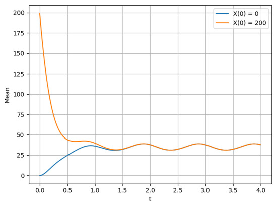
Figure 2. Average $E(t,k)$ for $t\in [0,4]$ at $N=200$.

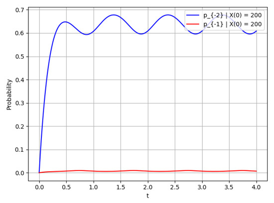
Figure 3. Probability $F,R$ for $t\in [0,4]$ and initial conditions $X\left(0\right)$ = 200 and $X\left(0\right)$ = 200, respectively.

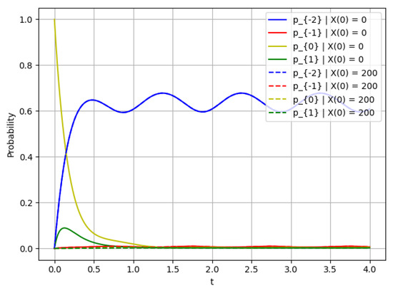
Figure 4. Probability $p_{-2}\left(t\right),p_{-1}\left(t\right),p_0\left(t\right),p_1\left(t\right)$ for $t\in [0,4]$; this figure shows the rate of convergence.

• The mathematical expectation of the number of customers in the system $E(t,k)$ for $t\in [0,4]$ and different initial conditions $X\left(0\right)=0$ and $X\left(0\right)=200$.
• The probability of states $F,R$ for $t\in [0,4]$ and $X\left(0\right)=200$.
• The probability $F,R$ and several operating states $p_0\left(t\right),p_1\left(t\right)$, at $t\in [0,4]$ and different initial conditions $X\left(0\right)=0$ (solid lines) and $X\left(0\right)=200$ (dashed lines).

For comparison, we present the corresponding graphs for a process with a small number of states for $N=10$, see Figure 5, Figure 6 and Figure 7.

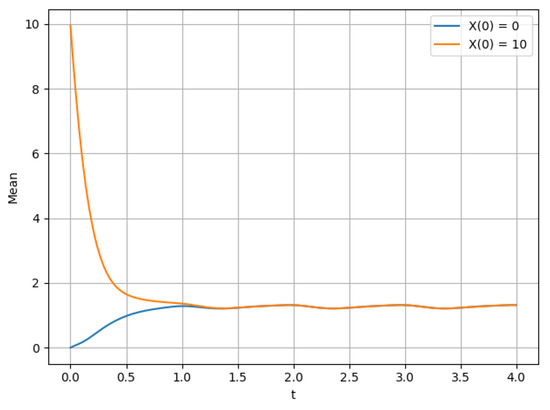
Figure 5. Average $E(t,k)$ for $t\in [0,4]$ at $N=10$.

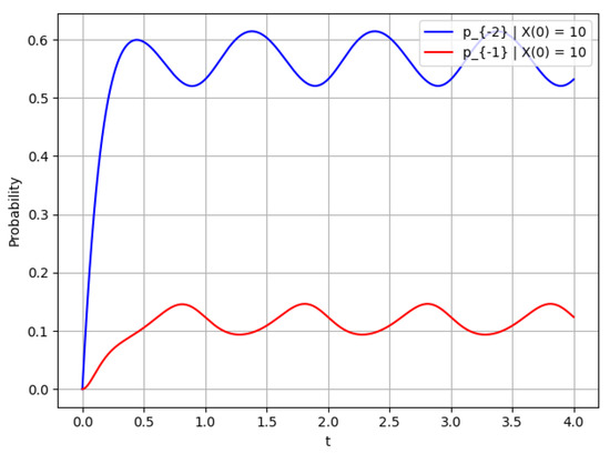
Figure 6. Probability $F,R$ for $t\in [0,4]$; this figure shows the rate of convergence.

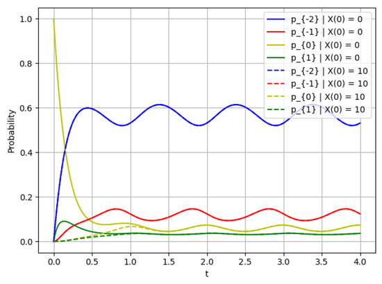
Figure 7. Probability $p_{-2}\left(t\right),p_{-1}\left(t\right),p_0\left(t\right),p_1\left(t\right)$ for $t\in [0,4]$; this figure shows the rate of convergence for $N=10$.

• The mathematical expectation of the number of customers in the system $E(t,k)$ for $t\in [0,4]$ and different initial conditions $X\left(0\right)=0$ and $X\left(0\right)=10$.
• The probability of states $F,R$ for $t\in [0,4]$ and $X\left(0\right)=10$.
• The probability $F,R$ and several operating states $p_0\left(t\right),p_1\left(t\right)$, at $t\in [0,4]$ and different initial conditions $X\left(0\right)=0$ (solid lines) and $X\left(0\right)=10$ (dashed lines).

Example 2.

Now, consider the ordinary Prendiville model with the finite state space $\{0,1,2\dots ,N\}$ for $N=200$. The corresponding queue-length process has no ’special’ states F and R.

Then, the transposed intensity matrix has the form

$$A\left(t\right)=\left(\begin{array}{cccc}-{\lambda }_0\left(t\right)& {\mu }_1\left(t\right)& \cdots & 0\\ {\lambda }_0\left(t\right)& -({\lambda }_1\left(t\right)+{\mu }_1\left(t\right))& \cdots & ⋮\\ 0& {\lambda }_1\left(t\right)& \ddots & 0\\ ⋮& ⋮& \cdots & {\mu }_N\left(t\right)\\ 0& \cdots & {\lambda }_{N-1}\left(t\right)& -{\mu }_N\left(t\right)\end{array}\right).$$

Let the intensities have the form

${\lambda }_k\left(t\right)=(N-k)\lambda \left(t\right)=(N-k)(2+sin2\pi t)$, if $k=0,1,\dots ,N$.

${\mu }_k\left(t\right)=k\mu \left(t\right)=k(7+1.5cos2\pi t)$, if $k=1,2,\dots ,N$.

This is an ordinary inhomogeneous birth–death process; the corresponding rate of convergence and limiting characteristics can be obtained in the same way as in [2]. We also consider two situations with $N=200$ and $N=10$, and the corresponding characteristics are shown in Figure 8, Figure 9, Figure 10 and Figure 11 and Figure 12, Figure 13, Figure 14 and Figure 15, respectively.

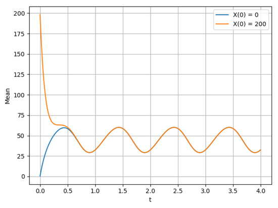
Figure 8. Average $E(t,k)$ for $t\in [0,4]$.

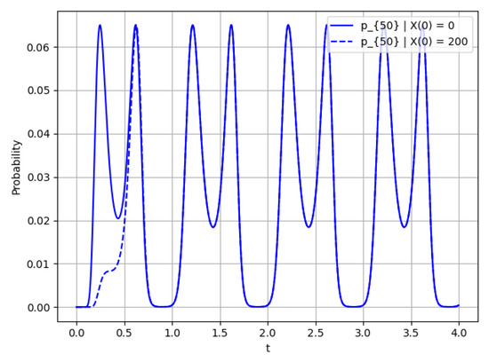
Figure 9. Probability $p_{50}\left(t\right),p_{51}\left(t\right)$ for $t\in [0,4]$; this figure shows the rate of convergence.

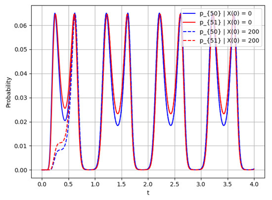
Figure 10. Probability $p_{50}\left(t\right),p_{51}\left(t\right)$ for $t\in [0,4]$; this figure shows the rate of convergence.

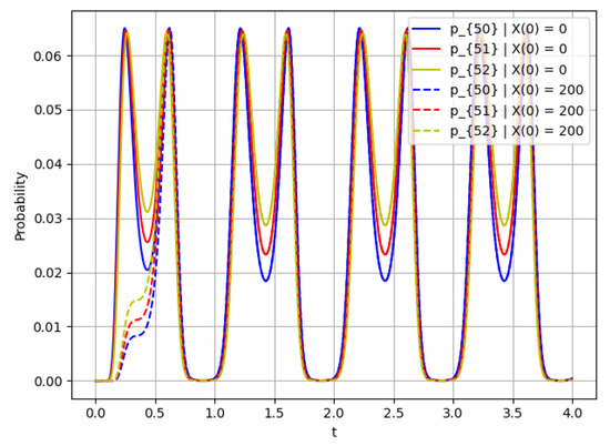
Figure 11. Probability $p_{50}\left(t\right),p_{51}\left(t\right),p_{52}\left(t\right)$ for $t\in [0,4]$; this figure shows the rate of convergence.

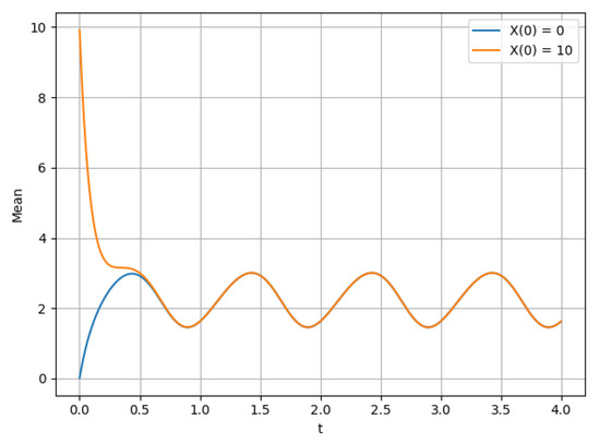
Figure 12. Average $E(t,k)$ for $t\in [0,4]$ at $N=10$.

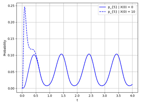
Figure 13. Probability $p_5\left(t\right)$ for $t\in [0,4]$; this figure shows the rate of convergence for $N=10$.

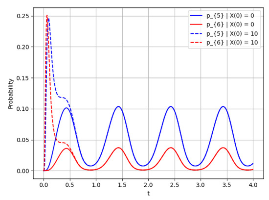
Figure 14. Probability $p_5\left(t\right),p_6\left(t\right)$ for $t\in [0,4]$; this figure shows the rate of convergence for $N=10$.

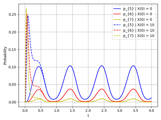
Figure 15. Probability $p_5\left(t\right),p_6\left(t\right),p_7\left(t\right)$ for $t\in [0,4]$; this figure shows the rate of convergence for $N=10$.

(a)

$N=200$

• The mathematical expectation of the number of customers in the system $E(t,k)$ for $t\in [0,4]$ and different initial conditions $X\left(0\right)=0$ and $X\left(0\right)=200$.
• The probability $p_{50}\left(t\right)$ for $t\in [0,4]$ and different initial conditions $X\left(0\right)=0$ (solid line) and $X\left(0\right)=200$ (dashed line).
• The probability $p_{50}\left(t\right),p_{51}\left(t\right)$ for $t\in [0,4]$ and different initial conditions $X\left(0\right)=0$ (solid lines) and $X\left(0\right)=200$ (dashed lines).
• The probability $p_{50}\left(t\right),p_{51}\left(t\right),p_{52}\left(t\right)$ for $t\in [0,4]$ and different initial conditions $X\left(0\right)=0$ (solid lines) and $X\left(0\right)=200$ (dashed lines).

(b)

$N=10$

• The mathematical expectation of the number of customers in the system $E(t,k)$ for $t\in [0,4]$ and different initial conditions $X\left(0\right)=0$ and $X\left(0\right)=10$.
• The probability $p_5\left(t\right)$ for $t\in [0,4]$ and different initial conditions $X\left(0\right)=0$ (solid line) and $X\left(0\right)=10$ (dashed line).
• The probability $p_5\left(t\right),p_6\left(t\right)$ for $t\in [0,4]$ and different initial conditions $X\left(0\right)=0$ (solid lines) and $X\left(0\right)=10$ (dashed lines).
• The probability $p_5\left(t\right),p_6\left(t\right),p_7\left(t\right)$ for $t\in [0,4]$ and different initial conditions $X\left(0\right)=0$ (solid lines) and $X\left(0\right)=10$ (dashed lines).

5. Conclusions

In this paper, a time-inhomogeneous Prendiville model with failures and repairs was studied. The property of weak ergodicity was considered, and estimates of the rate of convergence for the main probabilistic characteristics of the model were obtained. We used two approaches for this estimation: the elimination of the state with the minimum number, and the recently introduced so-called C-matrix method; the second method was more suitable, due to the special structure of the process intensity matrix, as shown in the examples. In addition, we briefly discussed stability estimates and the situation with proportional intensities.

References

- Ricciardi, L.M. Stochastic Population Theory: Birth and Death Processes. In Mathematical Ecology. Biomathematics; Hallam, T.G., Levin, S.A., Eds.; Springer: Berlin/Heidelberg, Germany, 1986; Volume 17, pp. 155–190. [Google Scholar] [CrossRef]
- Zeifman, A.; Satin, Y.; Kovalev, I.; Razumchik, R.; Korolev, V. Facilitating Numerical Solutions of Inhomogeneous Continuous Time Markov Chains Using Ergodicity Bounds Obtained with Logarithmic Norm Method. Mathematics. 2021, 9, 42. [Google Scholar] [CrossRef]
- Razumchik, R.; Rumyantsev, A. Some ergodicity and truncation bounds for a small scale Markovian supercomputer model. In Proceedings of the 36th ECMS International Conference on Modelling and Simulation ECMS 2022, Norway, Alesund, 30 May–3 June 2022. [Google Scholar] [CrossRef]
- Gnedenko, B.V.; Makarov, I.P. Properties of a problem with losses in the case of periodic intensities. Diff. Equs. 1971, 7, 1696–1698. [Google Scholar]
- Prendiville, B.J. Discussion Symposium on stochastic processes. J. R. Statist. Soc. B 1949, 11, 273. [Google Scholar]
- Takashima, M. Note on evolutionary processes. Bull. Math. Stat. 1956, 7, 18–24. [Google Scholar] [CrossRef]
- Giorno, V.; Negri, C.; Nobile, A.G. A solvable model for a finite capacity queueing system. Appl. Prob. 1985, 22, 903–911. [Google Scholar] [CrossRef]
- Karlin, S.; McGregor, J. Ehrenfest Urn Model. J. Appl. Prob. 1965, 2, 352–376. [Google Scholar] [CrossRef]
- Flegg, M.B.; Pollett, P.K.; Gramotnev, D.K. Ehrenfest model for condensation and evaporation processes in degrading aggregates with multiple bonds. Phys. Rev. 2008, 78, 031117. [Google Scholar] [CrossRef] [PubMed]
- Zheng, Q. Note on the non-homogeneous Prendiville process. Math. Biosci. 1998, 148, 1–5. [Google Scholar] [CrossRef]
- Giorno, V.; Nobile, A.G. Bell Polynomial Approach for Time-Inhomogeneous Linear Birth–Death Process with Immigration. Mathematics 2020, 8, 1123. [Google Scholar] [CrossRef]
- Mitrophanov, A.Y. Stability and exponential convergence of continuous-time Markov chains. J. Appl. Prob. 2003, 40, 970–979. [Google Scholar] [CrossRef]
- Giorno, V.; Nobile, A.G.; Spina, S. Some remarks on the prendiville model in the presence of jumps. In International Conference on Computer Aided Systems Theory, Proceedings of the 17th International Conference, Las Palmas de Gran Canaria, Spain, 17–22 February 2019; Springer: Cham, Switzerland, 2019; pp. 150–157. [Google Scholar] [CrossRef]
- Giorno, V.; Nobile, A.G. A Time-Inhomogeneous Prendiville Model with Failures and Repairs. Mathematics 2022, 10, 251. [Google Scholar] [CrossRef]
- Matis, J.H.; Kiffe, T.R. Stochastic Compartment models with Prendiville growth rates. Math. Biosci. 1996, 138, 31–43. [Google Scholar] [CrossRef]
- Parthasarathy, P.R.; Krishna Kumar, B. Stochastic Compartmental models with Prendiville growth mechanisms. Math. Biosci. 1995, 125, 51–60. [Google Scholar] [CrossRef]
- Zeifman, A.; Leorato, S.; Orsingher, E.; Satin, Y.; Shilova, G. Some universal limits for nonhomogeneous birth and death processes. Queueing Syst. 2006, 52, 139–151. [Google Scholar] [CrossRef]
- Satin, Y.A. On the bounds of the rate of convergence for Mt/Mt/1 model with two different requests. Syst. Means Inform. 2021, 31, 17–27. [Google Scholar] [CrossRef]
- Zeifman, A.I.; Satin, Y.A.; Korolev, V. Two Approaches to the Construction of Perturbation Bounds for Continuous-Time Markov Chains. Mathematics 2020, 8, 253. [Google Scholar] [CrossRef]
- Zeifman, A.I. Quasi-ergodicity for non-homogeneous continuous-time Markov chains. J. Appl. Probab. 1989, 26, 643–648. [Google Scholar] [CrossRef]
Publisher’s Note: MDPI stays neutral with regard to jurisdictional claims in published maps and institutional affiliations. |
© 2022 by the authors. Licensee MDPI, Basel, Switzerland. This article is an open access article distributed under the terms and conditions of the Creative Commons Attribution (CC BY) license (https://creativecommons.org/licenses/by/4.0/).