Approximating Common Fixed Points of Nonexpansive Mappings on Hadamard Manifolds with Applications

Abstract

The point of this research is to present a new iterative procedure for approximating common fixed points of nonexpansive mappings in Hadamard manifolds. The convergence theorem of the proposed method is discussed under certain conditions. For the sake of clarity, we provide some numerical examples to support our results. Furthermore, we apply the suggested approach to solve inclusion problems and convex feasibility problems.

1. Introduction

Let C be a nonempty, closed, and geodesic convex subset of a Hadamard manifold M. Assume that $g:C\to C$ is a nonexpansive mapping, which means that $d\left(g\right(x),g(y\left)\right)\le d(x,y)$ for every $x,y\in C$, where $d(·,·)$ stands for a Riemannian distance function. In this research, we consider the following fixed point problem:

$$\mathrm{find}{x}^{*}\in C\mathrm{such}\mathrm{that}g\left(x^{*}\right)=x^{*}.$$

(1)

$\mathcal{F}\left(g\right):\{x\in C:g(x)=x\}$ denotes the set of fixed points of the mapping g. Many problems, such as convex feasibility problems, convex optimization problems, monotone variational inequalities, and image restorations, can be cast in the light of fixed point problems for nonexpansive mappings, which leads to a wide range of specific applications (see [1,2,3,4] and references therein).

To estimate fixed points, there is a significant amount of literature on fixed point iteration approaches. Most of the research has focused on the case when g is a self-mapping defined on a convex subset C of a normed linear space, and here are some of the most famous variations:

1.

The Picard algorithm [5] is defined by

$$x_{n+1}=g\left(x_n\right),\forall n\in \mathbb{N}.$$

(2)

2.

The Mann algorithm [6] is defined by

$$x_{n+1}=a_n{x}_n+(1-a_n)g\left(x_n\right),\forall n\in \mathbb{N},$$

(3)

where $\left\{a_n\right\}$ is a sequence in $(0,1)$.

3.

The Ishikawa algorithm [7] is defined by

$$x_{n+1}=a_n{x}_n+(1-a_n)g[b_n{x}_n+(1-b_n)g\left(x_n\right)],\forall n\in \mathbb{N},$$

(4)

where $\left\{a_n\right\}$ and $\left\{b_n\right\}$ are sequences in $(0,1)$. One can see that the Ishikawa algorithm is a two-step Mann algorithm.

Assuming g is a contraction mapping, the sequence $\left\{x_n\right\}$ generated by Picard’s iteration (2) converges strongly to a unique fixed point. The Picard method may not converge if the mapping g is nonexpansive. On the other hand, the sequence $\left\{x_n\right\}$ produced by Mann’s iteration (3) converges weakly to a fixed point of the nonexpansive mapping g. Subsequently, numerous scholars have investigated the Mann method and the Ishikawa algorithm to estimate fixed points of nonexpansive mapping. Observe, for instance [8,9,10,11,12,13,14,15].

Both Sahu et al. [9] and Thakur et al. [10] published their findings in 2016, proposing the same iterative approach for approximating fixed points of nonexpansive mappings in uniformly convex Banach spaces:

$$\{\begin{array}{c}{z}_n=(1-c_n)x_n+c_{n}g\left(x_n\right),\hfill \\ y_n=(1-b_n)z_n+b_{n}g\left(z_n\right),\hfill \\ x_{n+1}=(1-a_n)g\left(z_n\right)+a_{n}g\left(y_n\right),\forall n\in \mathbb{N},\hfill \end{array}$$

(5)

where $\left\{a_n\right\},\left\{b_n\right\}$, and $\left\{c_n\right\}$ are sequences in $(0,1)$. The authors [9,10] showed that the iterative scheme (5) converges to fixed points of contractive mappings faster than various existing iterative schemes. Recently, the iterative method (5) has been an attractive process and has been extensively studied in many directions; see, e.g., Refs. [12,16,17,18]. In particular, Padcharoen and Sukprasert [12] improved and extended the iterative scheme (5) for finding common fixed points of two nonexpansive mappings $g,h:C\to C$, which is defined by the following:

$$\{\begin{array}{c}{z}_n=(1-c_n)x_n+c_{n}g\left(x_n\right),\hfill \\ y_n=(1-b_n)z_n+b_{n}h\left(z_n\right),\hfill \\ x_{n+1}=(1-a_n)g\left(z_n\right)+a_{n}h\left(y_n\right),\forall n\in \mathbb{N},\hfill \end{array}$$

(6)

where $\left\{a_n\right\},\left\{b_n\right\}$, and $\left\{c_n\right\}$ are sequences in $(0,1)$. The authors of [12] proved that the sequence $\left\{x_n\right\}$ achieved by (6) converges weakly to common fixed points. Moreover, they applied the proposed iteration to solve common solutions of accretive operators, convex constrained least square problems, convex minimization problems, and signal processing in Banach spaces.

In recent years, many scholars have turned their attention to nonlinear problems in nonlinear systems such as Hadamard manifolds and CAT(0) spaces [19,20,21,22,23,24,25,26]. Nonlinear problems naturally extend from linear spaces to Riemannian manifolds, which provides a range of advantages. For instance, non-convex problems can be transformed as convex problems by introducing an appropriate Riemannian metric, and constrained optimization problems can be approached in the same manner as unconstrained problems. In addition to this, Hadamard manifolds are suitable frameworks for the development of effective methods for the solution of realistic problems [27,28,29,30].

In 2010, Li et al. [11] investigated the fixed point problem (1) in the context of Hadamard manifolds. The Mann and Halpern methods were also extended from Euclidean spaces to Hadamard manifolds. Recently, S-iterative techniques for approximating common fixed points of two nonexpansive mappings in the setting of Hadamard manifolds were recently presented by Sahu et al. [13].

Algorithm 1 (S-iterative algorithm rank 2). 

Given$g,h:C\to C$are nonexpansive mappings and$\left\{x_n\right\}$is defined by

$$\left\{\begin{array}{c}{y}_n={exp}_{x_n}(1-b_n){exp}_{x_n}^{-1}g\left(x_n\right),\hfill \\ x_{n+1}={exp}_{h\left(x_n\right)}(1-a_n){exp}_{h\left(x_n\right)}^{-1}g\left(y_n\right),\forall n\in \mathbb{N},\hfill \end{array}\right.$$

(7)

where$\left\{a_n\right\}$, $\left\{b_n\right\}$are sequences in$(0,1)$and exp is an exponential mapping.

Algorithm 2 (S-iterative algorithm rank 3). 

Given$g,h:C\to C$are nonexpansive mappings and$\left\{x_n\right\}$is defined by

$$\left\{\begin{array}{c}{z}_n={exp}_{x_n}(1-c_n){exp}_{x_n}^{-1}g\left(x_n\right),\hfill \\ y_n={exp}_{h\left(x_n\right)}(1-b_n){exp}_{h\left(x_n\right)}^{-1}g\left(z_n\right),\hfill \\ x_{n+1}={exp}_{h\left(x_n\right)}(1-a_n){exp}_{h\left(x_n\right)}^{-1}g\left(y_n\right),\forall n\in \mathbb{N},\hfill \end{array}\right.$$

(8)

where$\left\{a_n\right\},\left\{b_n\right\}$and$\left\{c_n\right\}$are sequences in$(0,1)$.

It was shown by the authors [13] that any sequence produced by the suggested two algorithms converges to the common fixed points of nonexpansive maps. In addition, they provide numerical examples to support their assertions.

The goal of this paper is to provide a formal introduction to the iterative process (6) in terms of exponential mappings on Hadamard manifolds, building on the foundation laid in [11,12]. Under certain conditions, we establish the convergence theorem of our proposed method for common fixed points of two nonexpansive mappings. We provide some numerical examples to indicate how successful the proposed method is, and we compare it with some of the other methods that are already in use. In addition to this, we illustrate how the proposed method can be utilized to solve inclusion and convex feasibility problems in Hadamard manifolds.

The remainder of this paper is organized as follows: In Section 2, we present basic concepts and fundamental results in Riemannian geometry. In Section 3, we propose an iterative algorithm for finding common fixed points of nonexpansive mappings in Hadamard manifolds. We establish the convergence results of the proposed algorithm. In Section 4, we present some numerical experiments to demonstrate applications of the results in the present paper. Section 5 consists of applications to inclusion problems and convex feasibility problems in Hadamard manifolds. Finally, Section 6 provides a concise overview of the paper.

2. Preliminaries

In this section, we review the necessary terminology, concepts, properties, and results from Riemannian geometry that will be used in the rest of the paper. Readers may find references to it in a variety of textbooks that serve as introduction to Riemannian geometry. Some examples are [31,32,33].

Let us assume that M is a connected manifold with finite dimensions. The tangent bundle of M is defined by $TM={\bigcup }_{p\in M}{T}_{p}M$, where $T_{p}M$ is the tangent space of M at p and $\mathbf{0}$ denotes the zero section of $TM.$ Every manifold M is a Riemannian manifold if and only if it is endowed with a Riemannian metric ${⟨·,·⟩}_p$ with the corresponding norm denoted by ${\parallel ·\parallel }_p.$ If there is no doubt, the subscript p is omitted. Determine the length of the piecewise smooth curve $\phi :[a,b]\to M$ by using the formula $L\left(\phi \right)={\int }_a^b\parallel {\phi }^{{}^{\prime }}\left(t\right)\parallel dt,$ where ${\phi }^{{}^{\prime }}\left(t\right)$ is the tangent vector at $\phi \left(t\right)$ in the tangent space $T_{\phi \left(t\right)}M$. A Riemannian distance, indicated by $d(p,q)$, is the shortest path between any two points p and q.

Let ∇ be a Levi–Civita connection associated with the Riemannian manifold M. A smooth vector field V along a smooth curve $\phi$ is said to be parallel ⟺${\nabla }_{{\phi }^{{}^{\prime }}}V=\mathbf{0}$. If ${\phi }^{{}^{\prime }}$ is parallel to itself, we call it a geodesic, and in this case $\parallel {\phi }^{{}^{\prime }}\parallel$ is a constant. The curve $\phi$ is considered to be normalized when the value of $\parallel {\phi }^{{}^{\prime }}\parallel =1$. If the length of a geodesic that joins two points p and q in M is equal to the distance between those two points, then we refer to that geodesic as a minimizing geodesic.

If the geodesics of a Riemannian manifold can be determined for any value of $t\in \mathbb{R}$, then the manifold is said to be complete. The Hopf–Rinow theorem states that if M is complete, then any two points in M can be connected via a minimizing geodesic. In addition to this, because $(M,d)$ is a complete metric space, any bounded closed subset is a compact subset.

Let M be a complete Riemannian manifold and $p\in M$. The exponential map ${exp}_p:T_{p}M\to M$ is given by ${exp}_{p}u={\phi }_p(1,p)$, where $\phi (·)={\phi }_u(·,p)$ is the geodesic starting at the point p with velocity u (i.e., ${\phi }_u(0,p)=p$ and ${\phi }_u^{{}^{\prime }}(0,p)=p$). Then, for each real number t, we have ${exp}_{p}tu={\phi }_u(t,p)$ and ${exp}_p\mathbf{0}={\phi }_u(0,p)=p$. Note that exponential map is differentiable on $T_{p}M$ for each $p\in M$. This implies that the exponential map has an inverse ${exp}_p^{-1}:M\to T_{p}M$. We also have $d(p,q)=\parallel {exp}_p^{-1}q\parallel ,$$\forall p,q\in M$.

A complete simply connected Riemannian manifold of non-positive sectional curvature is named a Hadamard manifold. The remainder of the article will proceed on the assumption that M is a Hadamard manifold with finite dimensions. The exponential mapping ${exp}_p:T_{p}M\to M$ is a diffeomorphism for $p\in M$. Any two points $p,q\in M$ have a unique minimizing normalized geodesic connecting them ([31] Theorem 4.1).

A geodesic triangle $▵(p_1,p_2,p_3)$ of a Riemannian manifold M is a set consisting of three points $p_1$, $p_2$ and $p_3$, and three minimizing geodesics joining these points.

Proposition 1 

([31]).Let $▵(p_1,p_2,p_3)$ be a geodesic triangle. Then

$$d^2(p_1,p_2)+d^2(p_2,p_3)-2⟨{exp}_{p_2}^{-1}{p}_1,{exp}_{p_2}^{-1}{p}_3⟩\le d^2(p_3,p_1),$$

(9)

and

$$d^2(p_1,p_2)\le ⟨{exp}_{p_1}^{-1}{p}_3,{exp}_{p_1}^{-1}{p}_2⟩+⟨{exp}_{p_2}^{-1}{p}_3,{exp}_{p_2}^{-1}{p}_1⟩.$$

(10)

Moreover, if θ is the angle at $p_1$, then we have

$$⟨{exp}_{p_1}^{-1}{p}_2,{exp}_{p_1}^{-1}{p}_3⟩=d(p_2,p_1)d(p_1,p_3)cos\theta .$$

Readers can refer to [34] for further information on the relation between geodesic triangles on Riemannian manifolds and triangles on ${\mathbb{R}}^2$.

Lemma 1 

([34]).Let $▵(p_1,p_2,p_3)$ be a geodesic triangle in M. Then, there exists a triangle $▵(\overline{p_1},\overline{p_2},\overline{p_3})$ for $▵(p_1,p_2,p_3)$ such that $d(p_i,p_{i+1})=\parallel \overline{p_i}-\overline{p_{i+1}}\parallel$, indices taken modulo 3; it is unique up to an isometry of ${\mathbb{R}}^2$.

The triangle $▵(\overline{p_1},\overline{p_2},\overline{p_3})$ in Lemma 1 is said to be a comparison triangle for $▵(p_1,p_2,p_3)$. The points $\overline{p_1}$, $\overline{p_2}$, $\overline{p_3}$ are called comparison points to the points $p_1,p_2,p_3,$ respectively.

Lemma 2. 

Let $▵(p_1,p_2,p_3)$ be a geodesic triangle in M and $▵(\overline{p_1},\overline{p_2},\overline{p_3})$ be its comparison triangle.

(i)

Let ${\theta }_1,{\theta }_2,{\theta }_3$ (respectively, $\overline{{\theta }_1},\overline{{\theta }_2},\overline{{\theta }_3}$) be the angles of $▵(p_1,p_2,p_3)$ (respectively, $▵(\overline{p_1},\overline{p_2},\overline{p_3})$) at the vertices $p_1,p_2,p_3$ (respectively, $\overline{p_1}$, $\overline{p_2}$, $\overline{p_3}$). Then

$${\theta }_1\le \overline{{\theta }_1},{\theta }_2\le \overline{{\theta }_2}\mathrm{and}{\theta }_3\le \overline{{\theta }_3}.$$

(ii)

Let q be a point on the geodesic joining $p_1$ to $p_2$ and $\overline{q}$ its comparison point in the interval $[p_1,p_2]$. If $d(p_1,q)=\parallel \overline{p_1}-\overline{q}\parallel$ and $d(p_2,q)=\parallel \overline{p_2}-\overline{q}\parallel$, then $d(p_3,q)\le \parallel \overline{p_3}-\overline{q}\parallel$.

Several convex analysis concepts and results have been extended in the setting of manifolds. We present some of these that will be used throughout the rest of the paper.

Let M be an Hadamard manifold. A set $C\subset M$ is called geodesic convex if for any two points p and q in C, the geodesic joining p to q is contained in C; that is, if $\phi :[a,b]\to M$ is a geodesic such that $p=\phi \left(a\right)$ and $q=\phi \left(b\right)$, then $\phi (ta+(1-t\left)b\right)\in C,$ $\forall a,b\in \mathbb{R}$ and $t\in [0,1]$. A real valued function $f:M\to \mathbb{R}$ is called geodesic convex if for any geodesic $\phi :[a,b]\to M$ the composition function $f\circ \phi :[a,b]\to \mathbb{R}$ is convex; that is,

$$(f\circ \phi )(at+(1-t\left)b\right)\le t(f\circ \phi )\left(a\right)+(1-t)(f\circ \phi )\left(b\right),\forall a,b\in \mathbb{R}\mathrm{and}t\in [0,1].$$

Proposition 2 

([31]).Let the distance function be $d:M\times M\to \mathbb{R}$. Then, $d(·,·)$ is a geodesic convex function with respect to the Riemannian metric product; that is, the following inequality holds for any pair of geodesics ${\phi }_1:[0,1]\to M$ and ${\phi }_2:[0,1]\to M$.

$$d({\phi }_1\left(t\right),{\phi }_2\left(t\right))\le (1-t)d({\phi }_1\left(0\right),{\phi }_2\left(0\right))+td({\phi }_1\left(1\right),{\phi }_2\left(1\right)),\forall t\in [0,1].$$

In particular, for each $q\in M$, the function $d(·,q):M\to \mathbb{R}$ is a geodesic convex.

Let us conclude this section with the following results, which are essential to proving our convergence theorem.

Definition 1 

([20]).Assume that $\left\{p_n\right\}$ is a sequence in M and that C is a nonempty subset of M. If $d(p_{n+1},q)\le d(p_n,q),$$\forall q\in C$ and $n\in \mathbb{N}$, then $\left\{p_n\right\}$ is Fejér monotone with respect to C.

Lemma 3 

([20]).Let C be a nonempty subset of M and $\left\{p_n\right\}\subset M$ be a sequence in M, such that $\left\{p_n\right\}$ is a Fejér monotone with respect to C. Then, the following holds:

(i)

For every $q\in C$, $\left\{d(p_n,q)\right\}$ converges;

(ii)

$\left\{p_n\right\}$ is bounded;

(iii)

Assume that any cluster point of $\left\{p_n\right\}$ belongs to C, then $\left\{p_n\right\}$ converges to a point in C.

3. Main Results

Unless otherwise stated, the rest of this article will refer to C in terms of a nonempty, closed, and geodesic convex subset of a Hadamard manifold $M.$ Given two mappings g and h from C to C, we say that g and h have at least one fixed point. The common fixed points between mappings g and h are denoted $\mathsf{\Gamma }(g,h):=\mathcal{F}\left(g\right)\cap \mathcal{F}\left(h\right)$. An iterative approach for finding common fixed points of two nonexpansive mappings g and h is described below.

Algorithm 3. 

Let$g,h:C\to C$are mappings, and$x_0\in C$be an initial point. Given$x_n\in C$and calculate$x_{n+1}$by

$$\begin{array}{ccc}\hfill z_n& =& {exp}_{x_n}{c}_n{exp}_{x_n}^{-1}g\left(x_n\right),\hfill \end{array}$$

(11)

$$\begin{array}{ccc}\hfill y_n& =& {exp}_{z_n}{b}_n{exp}_{z_n}^{-1}h\left(z_n\right),\hfill \end{array}$$

(12)

$$\begin{array}{ccc}\hfill x_{n+1}& =& {exp}_{g\left(z_n\right)}{a}_n{exp}_{g\left(z_n\right)}^{-1}h\left(y_n\right),\forall n\in \mathbb{N},\hfill \end{array}$$

(13)

where$\left\{a_n\right\},$$\left\{b_n\right\}$and$\left\{c_n\right\}$are real positive sequences in$(0,1)$.

Following this, we are going to prove that Algorithm 3 satisfies the conditions required to achieve the convergence theorem.

Theorem 1. 

Let C be a nonempty, closed and geodesic convex subset of a Hadamard manifold M, and $g,h:C\to C$ are nonexpansive mappings such that $\mathsf{\Gamma }(g,h)\ne \varnothing$. Suppose that $\left\{a_n\right\},$$\left\{b_n\right\}$ and $\left\{c_n\right\}$ are real positive sequences satisfying $0<k_1\le a_n\le \widehat{k_1}<1,0<k_2\le b_n\le \widehat{k_2}<1$ and $0<k_3\le c_n\le \widehat{k_3}<1,$ $\forall n\in \mathbb{N}$. Let $x_0\in C$ and $\left\{x_n\right\}$ is defined by Algorithm 3. Then $\left\{x_n\right\}$ converges to a common fixed point of g and h.

Proof. 

Because $(M,d)$ is a complete metric space and $\mathsf{\Gamma }(g,h)\subseteq M$, it is sufficient to show by Lemma 3 that $\left\{x_n\right\}$ is Fejér monotone with respect to $\mathsf{\Gamma }(g,h)$ and the cluster point of $\left\{x_n\right\}$ belongs to $\mathsf{\Gamma }(g,h)$.

Fix $n\in \mathbb{N}$, let $\eta \in \mathsf{\Gamma }(g,h)$ and ${\phi }_1:[0,1]\to M$ be geodesic connecting $g\left(z_n\right)$ to $h\left(y_n\right)$, ${\phi }_2:[0,1]\to M$ be geodesic connecting $z_n$ to $h\left(z_n\right)$ and ${\phi }_3:[0,1]\to M$ be geodesic connecting $x_n$ to $g\left(x_n\right)$. Hence, (11), (12) and (13) can be written as $z_n={\phi }_3\left(c_n\right),y_n={\phi }_2\left(b_n\right)$ and $x_{n+1}={\phi }_1\left(a_n\right)$, respectively. By applying the geodesic convexity of the Riemannian distance, we have arrived at the conclusion that

$$\begin{array}{ccc}\hfill d(z_n,\eta )& =& d({\phi }_3\left(c_n\right),\eta )\hfill \\ & \le & (1-c_n)d(x_n,\eta )+c_{n}d(g\left(x_n\right),\eta )\hfill \\ & \le & (1-c_n)d(x_n,\eta )+c_{n}d(x_n,\eta )\hfill \\ & =& d(x_n,\eta ),\hfill \end{array}$$

(14)

$$\begin{array}{ccc}\hfill d(y_n,\eta )& =& d({\phi }_2\left(b_n\right),\eta )\hfill \\ & \le & (1-b_n)d(z_n,\eta )+b_{n}d(h\left(z_n\right),\eta )\hfill \\ & \le & (1-b_n)d(z_n,\eta )+b_{n}d(z_n,\eta )\hfill \\ & =& d(z_n,\eta )\hfill \\ & \le & d(x_n,\eta ),\hfill \end{array}$$

(15)

and

$$\begin{array}{ccc}\hfill d(x_{n+1},\eta )& =& d({\phi }_1\left(a_n\right),\eta )\hfill \\ & \le & (1-a_n)d(g\left(z_n\right),\eta )+a_{n}d(h\left(y_n\right),\eta )\hfill \\ & \le & (1-a_n)d(z_n,\eta )+a_{n}d(y_n,\eta )\hfill \\ & \le & (1-a_n)d(x_n,\eta )+a_{n}d(x_n,\eta )\hfill \\ & =& d(x_n,\eta ).\hfill \end{array}$$

(16)

As a result, $\left\{x_n\right\}$ is a Fejér monotone with respect to $\mathsf{\Gamma }(g,h)$. Lemma 3 (ii) states that $\left\{x_n\right\}$ is bounded. Therefore, there is a subsequence $\left\{x_{n_i}\right\}$ of $\left\{x_n\right\}$ that converges to a cluster point p. Following this, we will prove that

$$\underset{n\to +\infty }{lim}d(x_n,h\left(x_n\right))=0.$$

Fix $n\in \mathbb{N}$ and for $\eta \in \mathsf{\Gamma }(g,h)$. Let $▵(g\left(z_n\right),h\left(y_n\right),\eta )\subseteq M$ be a geodesic triangle with vertices $g\left(z_n\right)$, $h\left(y_n\right)$ and $\eta$, and $▵\left(\overline{g\left(z_n\right)},\overline{h\left(y_n\right)},\overline{\eta }\right)\subseteq {\mathbb{R}}^2$ be the corresponding comparison triangle. Then, we obtain $d(g\left(z_n\right),\eta )=∥\overline{g\left(z_n\right)}-\overline{\eta }∥,d(h\left(y_n\right),\eta )=∥\overline{h\left(y_n\right)}-\overline{\eta }∥$ and $d(g\left(z_n\right),h\left(y_n\right))=∥\overline{g\left(z_n\right)}-\overline{h\left(y_n\right)}∥.$ Let $\overline{x_{n+1}}=(1-a_n)\overline{g\left(z_n\right)}+a_n\overline{h\left(y_n\right)}$ be the comparison point of $x_{n+1}$. Using (ii) of Lemma 2 together with the expressions (14) and (15),

$$\begin{array}{ccc}\hfill d^2(x_{n+1},\eta )& \le & \parallel \overline{x_{n+1}}-\overline{\eta }{\parallel }^2\hfill \\ & =& {∥(1-a_n)\overline{g\left(z_n\right)}+a_n\overline{h\left(y_n\right)}-\overline{\eta }∥}^2\hfill \\ & =& (1-a_n){∥\overline{g\left(z_n\right)}-\overline{\eta }∥}^2+a_n{∥\overline{h\left(y_n\right)}-\overline{\eta }∥}^2-a_n(1-a_n){∥\overline{g\left(z_n\right)}-\overline{h\left(y_n\right)}∥}^2\hfill \\ & =& (1-a_n)d^2\left(g\left(z_n\right),\eta \right)+a_n{d}^2(h\left(y_n\right),\eta )-a_n(1-a_n)d^2(g\left(z_n\right),h\left(y_n\right))\hfill \\ & \le & (1-a_n)d^2\left(z_n,\eta \right)+a_n{d}^2(y_n,\eta )-a_n(1-a_n)d^2(g\left(z_n\right),h\left(y_n\right))\hfill \\ & =& d^2(x_n,\eta )-a_n(1-a_n)d^2(g\left(z_n\right),h\left(y_n\right)),\forall n\in \mathbb{N},\hfill \end{array}$$

(17)

which implies that

$$a_n(1-a_n)d^2(g\left(z_n\right),h\left(y_n\right))\le d^2(x_n,\eta )-d^2(x_{n+1},\eta ),\forall n\in \mathbb{N}.$$

(18)

Based on the fact that $0<k_1\le a_n\le \widehat{k_1}<1$, so $k_1(1-\widehat{k_1})\le a_n(1-a_n),$ $\forall n\in \mathbb{N}.$ Summing up (18) from $j=0$ to $j=n$, we obtain

$$k_1(1-\widehat{k_1})\sum _{j=0}^n{d}^2(g\left(z_j\right),h\left(y_j\right))\le d^2(x_0,\eta )-d^2(x_{n+1},\eta ),\forall n\in \mathbb{N}.$$

Letting $n\to +\infty$, we have

$$k_1(1-\widehat{k_1})\sum _{j=0}^{+\infty }{d}^2(g\left(z_j\right),h\left(y_j\right))\le d^2(x_0,\eta )<+\infty .$$

Hence,

$$\underset{n\to +\infty }{lim}d(g\left(z_n\right),h\left(y_n\right))=0.$$

(19)

Now, let $▵(z_n,h\left(z_n\right),\eta )\subseteq M$ be a geodesic triangle with vertices $z_n$, $h\left(z_n\right)$ and $\eta$, and $▵\left(\overline{z_n},\overline{h\left(z_n\right)},\overline{\eta }\right)\subseteq {\mathbb{R}}^2$ be the corresponding comparison triangle. Then, we obtain

$$d(z_n,\eta )=∥\overline{z_n}-\overline{\eta }∥,d(h\left(z_n\right),\eta )=∥\overline{h\left(z_n\right)}-\overline{\eta }∥\mathrm{and}d(z_n,h\left(z_n\right))=∥\overline{z_n}-\overline{h\left(z_n\right)}∥.$$

Let $\overline{y_n}=(1-b_n)\overline{z_n}+b_n\overline{h\left(z_n\right)}$ be the comparison point of $y_n$. Using (ii) of Lemma 2 and (14), then

$$\begin{array}{ccc}\hfill d^2(y_n,\eta )& \le & \parallel \overline{y_n}-\overline{\eta }{\parallel }^2\hfill \\ & =& {∥(1-b_n)\overline{z_n}+b_n\overline{h\left(z_n\right)}-\overline{\eta }∥}^2\hfill \\ & =& (1-b_n){∥\overline{z_n}-\overline{\eta }∥}^2+b_n{∥\overline{h\left(z_n\right)}-\overline{\eta }∥}^2-b_n(1-b_n){∥\overline{z_n}-\overline{h\left(z_n\right)}∥}^2\hfill \\ & =& (1-b_n)d^2\left(z_n,\eta \right)+b_n{d}^2(h\left(z_n\right),\eta )-b_n(1-b_n)d^2(z_n,h\left(z_n\right))\hfill \\ & \le & (1-b_n)d^2\left(z_n,\eta \right)+b_n{d}^2(z_n,\eta )-b_n(1-b_n)d^2(z_n,h\left(z_n\right))\hfill \\ & =& d^2(z_n,\eta )-b_n(1-b_n)d^2(z_n,h\left(z_n\right))\hfill \\ & \le & d^2(x_n,\eta )-b_n(1-b_n)d^2(z_n,h\left(z_n\right)),\forall n\in \mathbb{N}.\hfill \end{array}$$

(20)

Adding (20) into (17) and using (14), we get

$$\begin{array}{ccc}\hfill d^2(x_{n+1},\eta )& \le & (1-a_n)d^2\left(z_n,\eta \right)+a_n[d^2(x_n,\eta )-b_n(1-b_n)d^2(z_n,h\left(z_n\right))]\hfill \\ & & -a_n(1-a_n)d^2(g\left(z_n\right),h\left(y_n\right))\hfill \\ & \le & d^2\left(x_n,\eta \right)-a_n{b}_n(1-b_n)d^2(z_n,h\left(z_n\right))-a_n(1-a_n)d^2(g\left(z_n\right),h\left(y_n\right)).\hfill \end{array}$$

(21)

Note that $k_1{k}_2(1-\widehat{k_2})\le a_n{b}_n(1-b_n)$. Summing up (21) form $j=0$ to $j=n$, we obtain

$$k_1{k}_2(1-\widehat{k_2})\sum _{j=0}^n{d}^2(z_n,h\left(z_n\right))\le d^2\left(x_0,\eta \right)-d^2\left(x_{n+1},\eta \right),\forall n\in \mathbb{N}.$$

Taking $n\to +\infty$, yields

$$k_1{k}_2(1-\widehat{k_2})\sum _{j=0}^{+\infty }{d}^2(z_n,h\left(z_n\right))\le d^2\left(x_0,\eta \right)<+\infty .$$

Therefore,

$$\underset{n\to +\infty }{lim}d(z_n,h\left(z_n\right))=0.$$

(22)

Moreover, let $▵(x_n,g\left(x_n\right),\eta )\subseteq M$ represent a geodesic triangle with vertices $x_n$, $g\left(x_n\right)$ and $\eta$, and $▵\left(\overline{x_n},\overline{g\left(x_n\right)},\overline{\eta }\right)\subseteq {\mathbb{R}}^2$ be the corresponding comparison triangle. Then, we get

$$d(x_n,\eta )=∥\overline{x_n}-\overline{\eta }∥,d(g\left(x_n\right),\eta )=∥\overline{g\left(x_n\right)}-\overline{\eta }∥\mathrm{and}d(x_n,g\left(x_n\right))=∥\overline{x_n}-\overline{g\left(x_n\right)}∥.$$

Let $\overline{z_n}=(1-c_n)\overline{x_n}+c_n\overline{g\left(x_n\right)}$ be the comparison point of $z_n$. Using (ii) of Lemma 2, then

$$\begin{array}{ccc}\hfill d^2(z_n,\eta )& \le & \parallel \overline{z_n}-\overline{\eta }{\parallel }^2\hfill \\ & =& {∥(1-c_n)\overline{x_n}+c_n\overline{g\left(x_n\right)}-\overline{\eta }∥}^2\hfill \\ & =& (1-c_n){∥\overline{x_n}-\overline{\eta }∥}^2+c_n{∥\overline{g\left(x_n\right)}-\overline{\eta }∥}^2-c_n(1-c_n){∥\overline{x_n}-\overline{g\left(x_n\right)}∥}^2\hfill \\ & =& (1-c_n)d^2\left(x_n,\eta \right)+c_n{d}^2(g\left(x_n\right),\eta )-c_n(1-c_n)d^2(x_n,g\left(x_n\right))\hfill \\ & \le & (1-c_n)d^2\left(x_n,\eta \right)+b_n{d}^2(x,\eta )-c_n(1-c_n)d^2(x_n,g\left(x_n\right))\hfill \\ & =& d^2(x_n,\eta )-c_n(1-c_n)d^2(x_n,g\left(x_n\right)),\forall n\in \mathbb{N}.\hfill \end{array}$$

(23)

Combining (23) and (17), and using (15), yields

$$\begin{array}{ccc}\hfill d^2(x_{n+1},\eta )& \le & (1-a_n)[d^2(x_n,\eta )-c_n(1-c_n)d^2(x_n,g\left(x_n\right))]+a_n{d}^2(y_n,\eta )\hfill \\ & & -a_n(1-a_n)d^2(g\left(z_n\right),h\left(y_n\right))\hfill \\ & \le & d^2(x_n,\eta )-(1-a_n)c_n(1-c_n)d^2(x_n,g\left(x_n\right))-a_n(1-a_n)d^2(g\left(z_n\right),h\left(y_n\right)).\hfill \end{array}$$

(24)

Note that $(1-\widehat{k_1})k_3(1-\widehat{k_3})\le (1-a_n)c_n(1-c_n)$. Taking the sum of (24) from $j=0$ to $j=n$, we get

$$(1-\widehat{k_1})k_3(1-\widehat{k_3})\sum _{j=0}^n{d}^2(x_n,g\left(x_n\right))\le d^2\left(x_0,\eta \right)-d^2\left(x_{n+1},\eta \right),\forall n\in \mathbb{N}.$$

Letting $n\to +\infty$, we have

$$(1-\widehat{k_1})k_3(1-\widehat{k_3})\sum _{j=0}^{+\infty }{d}^2(x_n,g\left(x_n\right))\le d^2\left(x_0,\eta \right)<+\infty .$$

This indicates that

$$\underset{n\to +\infty }{lim}d(x_n,g\left(x_n\right))=0.$$

(25)

With the help of the geodesic convexity of the Riemannian distance,

$$\begin{array}{ccc}\hfill d(z_n,x_n)& \le & (1-c_n)d(x_n,x_n)+c_{n}d(g\left(x_n\right),x_n)\hfill \\ & =& c_{n}d(g\left(x_n\right),x_n)\hfill \\ & \le & d(g\left(x_n\right),x_n).\hfill \end{array}$$

Taking $n\to +\infty$ into the last inequality and applying (25), we get

$$\underset{n\to +\infty }{lim}d(x_n,z_n)=0.$$

(26)

Because g is nonexpansive, then

$$\begin{array}{ccc}\hfill d(z_n,g\left(z_n\right))& \le & d(z_n,x_n)+d(x_n,g\left(x_n\right))+d(g\left(x_n\right),g\left(z_n\right))\hfill \\ & \le & d(x_n,z_n)+d(x_n,g\left(x_n\right))+d(x_n,z_n).\hfill \end{array}$$

In view of (25) and (26), we deduce that

$$\underset{n\to +\infty }{lim}d(z_n,g\left(z_n\right))=0.$$

(27)

Recall (12) that $y_n={exp}_{z_n}{b}_n{exp}_{z_n}^{-1}h\left(z_n\right)$, we get

$$d(y_n,z_n)=b_{n}d(z_n,h\left(z_n\right))\le d(z_n,h\left(z_n\right)).$$

Letting $n\to +\infty$ to the above inequality and using (22), so

$$\underset{n\to +\infty }{lim}d(y_n,z_n)=0.$$

(28)

Now,

$$\begin{array}{ccc}\hfill d(x_n,h\left(x_n\right))& \le & d(x_n,z_n)+d(z_n,g\left(z_n\right))+d(g\left(z_n\right),h\left(y_n\right))+d(h\left(y_n\right),h\left(z_n\right))\hfill \\ & & +d(h\left(z_n\right),h\left(x_n\right))\hfill \\ & \le & d(x_n,z_n)+d(z_n,g\left(z_n\right))+d(g\left(z_n\right),h\left(y_n\right))+d(y_n,z_n)+d(x_n,z_n).\hfill \end{array}$$

(29)

By taking $n\to +\infty$ into (29). Then, by combining (19), (26), (27) and (28),

$$\begin{array}{ccc}\hfill \underset{n\to +\infty }{lim}d(x_n,h\left(x_n\right))& \le & 2\underset{n\to +\infty }{lim}d(x_n,z_n)+\underset{n\to +\infty }{lim}d(z_n,g\left(z_n\right))+\underset{n\to +\infty }{lim}d(g\left(z_n\right),h\left(y_n\right))\hfill \\ & & +\underset{n\to +\infty }{lim}d(y_n,z_n)\hfill \\ & =& 0.\hfill \end{array}$$

(30)

Consider,

$$\begin{array}{ccc}\hfill d(p,g(p\left)\right)& \le & d(p,x_{n_i})+d(x_{n_i},g\left(x_{n_i}\right))+d(g\left(x_{n_i}\right),g\left(p\right))\hfill \\ & \le & 2d(p,x_{n_i})+d(x_{n_i},g\left(x_{n_i}\right)),\hfill \end{array}$$

and

$$\begin{array}{ccc}\hfill d(p,h(p\left)\right)& \le & d(p,x_{n_i})+d(x_{n_i},h\left(x_{n_i}\right))+d(h\left(x_{n_i}\right),h\left(p\right))\hfill \\ & \le & 2d(p,x_{n_i})+d(x_{n_i},h\left(x_{n_i}\right)).\hfill \end{array}$$

By letting $i\to +\infty$, we are able to show that $d(p,g(p\left)\right)=0$ and $d(p,h(p\left)\right)=0$. This proves that $p\in \mathsf{\Gamma }(g,h)$. According to Lemma 3 (iii), the sequence $\left\{x_n\right\}$ generated by Algorithm 3 converges to a common fixed point of g and h. As a result, the proof has been completed.    □

4. Numerical Examples

We provide two numerical examples on Hadamard manifolds in order to illustrate the performance of Algorithm 3 and to evaluate its efficacy in comparison to other existing algorithms. All programs were coded in Matlab R2016b, and the computations were done on a personal computer with an Intel(R) Core(TM) i7 @1.80 GHz, together with 8 GB 1600 MHz DDR3.

Example 1. 

Let $M=({\mathbb{R}}^3,⟨·,·⟩)$ be an Hadamard manifold with Riemannian metric $⟨u,v⟩=u^{\top }W\left(x\right)v,$ $\forall u,v\in T_{x}M$ and $\forall x=(x_1,x_2,x_3)\in M$, where $W\left(x\right)$ is $3\times 3$ matrix defined by

$$W\left(x\right):=\left(\begin{array}{ccc}1& 0& 0\\ 0& 1+4x_2^2& -2x_2\\ 0& -2x_2& 1\end{array}\right),\forall x\in M.$$

The Riemannian distance between any x and y in M is defined by

$$d^2(x,y)=\sum _{i=1}^2{(x_i-y_i)}^2+{(x_2^2-x_3-y_2^2+y_3)}^2.$$

See [28] for further details. The geodesic joining the points $\phi \left(0\right)=x$ and $\phi \left(1\right)=y$ is given by

$$\phi \left(t\right):=({\phi }_1\left(t\right),{\phi }_2\left(t\right),{\phi }_3\left(t\right)),\forall t\in [0,1],$$

where ${\phi }_i\left(t\right)=x_i+t(y_i-x_i)$, $\forall i=1,2$ and

$${\phi }_3\left(t\right)=x_3+t((y_3-x_3)-2{(y_2-x_2)}^2)+2t^2{(y_2-x_2)}^2.$$

Therefore, ${exp}_x\left(tv\right)=\phi \left(t\right),$ where $\phi :\mathbb{R}\to M$ is the unique geodesic starting from $\phi \left(0\right)=x$ with $v={\phi }^{{}^{\prime }}\left(0\right)\in T_{x}M$. To define the inverse exponential mapping, we use the following formula:

$${exp}_x^{-1}y=\left(y_1-x_1,y_2-x_2,y_3-x_3-{(y_2-x_2)}^2\right).$$

In the same vein as [35] [Example 5.1], we define two nonexpansive mappings $g,h:M\to M$ by

$$g\left(x\right)=(-x_1,-x_2,x_3),\forall x\in M,$$

and

$$h\left(x\right)=\left(\frac{x_1}{2},\frac{x_2}{3},\frac{x_3}{2}+\frac{x_2^2}{2}\right),\forall x\in M.$$

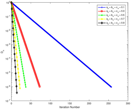
Then, $\mathcal{F}\left(g\right)=\{(x_1,x_2,x_3)\in M:x_1=x_2=0\}$ and $\mathcal{F}\left(h\right)=\left\{\right(0,0,0\left)\right\}$. These imply that $\mathsf{\Gamma }(g,h)=\left\{\right(0,0,0\left)\right\}$. Let $x^{*}=(0,0,0)$ and the initial point $x_0=(0,0,1)$. Denoted $D_n=d(x_n,x^{*})<{10}^{-6}$ as the stopping criterion. The five different cases of control parameters $a_n,b_n$ and $c_n$ are as follows:

$\begin{array}{cc}CaseI:\hfill & a_n=b_n=c_n=0.1.\hfill \\ CaseII:\hfill & a_n=b_n=c_n=0.3.\hfill \\ CaseIII:\hfill & a_n=b_n=c_n=0.5.\hfill \\ CaseIV:\hfill & a_n=b_n=c_n=0.7.\hfill \\ CaseV:\hfill & a_n=b_n=c_n=0.9.\hfill \end{array}$

The numerical behavior of Algorithm 3 using different choices of control parameters is reported in Table 1 and Figure 1.

Table 1. Numerical experiments of Example 1.

Case	Iteration	Time (s)
I	258	0.0291
II	74	0.0149
III	38	0.0115
IV	23	0.1060
V	16	0.0052

Figure 1. Numerical behaviour of $\left\{D_n\right\}$ for Example 1.

Remark 1. 

(i) 

Table 1 shows that Algorithm 3 with different choices of control parameters is efficient and simple to implement. The most essential point is that Algorithm 3 converges quickly when the control parameter are $0.5\le a_n,b_n,c_n<1$.

(ii) 

The speed of our proposed Algorithm 3 with the parameter $a_n=b_n=c_n=0.9$ is clearly faster than others, as can be seen in Figure 1.

Example 2. 

Let $M:={\mathbb{H}}^3=\{x=(x_1,x_2,x_3,x_4)\in {\mathbb{R}}^4:⟨x,x⟩=-1,x_4>0\}$ be the 3−dimensional hyperbolic space endowed with the Lorentz metric $⟨·,·⟩$ of ${\mathbb{R}}^4$ defined by

$$⟨x,y⟩=x_1{y}_1+x_2{y}_2+x_3{y}_3-x_4{y}_4,x=(x_1,x_2,x_3,x_4),y=(y_1,y_2,y_3,y_4)\in {\mathbb{H}}^3.$$

For richer details, see [36,37]. Then, ${\mathbb{H}}^3$ is a Hadamard manifold with sectional curvature $-1$. The normalized geodesic $\phi :\mathbb{R}\to {\mathbb{H}}^3$ starting from $x\in {\mathbb{H}}^3$ is defined as

$$\phi \left(t\right)=(cosht)x+(sinht)v,\forall t\in \mathbb{R},$$

where $v\in T_x{\mathbb{H}}^3$ is unit vector. In light of this, we deduce that ${exp}_{x}tv=(cosht)x+(sinht)v.$ The inverse exponential map is assigned by

$${exp}_x^{-1}y=\mathrm{arccosh}(-⟨x,y⟩){\displaystyle \frac{y+⟨x,y⟩x}{\sqrt{{⟨x,y⟩}^2-1}}},\forall x,y\in {\mathbb{H}}^3.$$

The Riemannian distance $d:{\mathbb{H}}^3\times {\mathbb{H}}^3\to \mathbb{R}$ is defined by $d(x,y)=\mathrm{arccosh}(-⟨x,y⟩)$.

Let $g,h:{\mathbb{H}}^3\to {\mathbb{H}}^3$ are nonexpansive mappings respectively defined by

$$g(x_1,x_2,x_3,x_4)=(-x_1,-x_2,-x_3,x_4),$$

and

$$h(x_1,x_2,x_3,x_4)=(-x_1,x_2,x_3,x_4)$$

for all $x=(x_1,x_2,x_3,x_4)\in {\mathbb{H}}^3.$ Then, $\mathcal{F}\left(g\right)=\left\{\right(0,0,0,1\left)\right\}$ and $\mathcal{F}\left(h\right)=\{(x_1,x_2,x_3,x_4)\in {\mathbb{H}}^3:x_1=0,x_2^2+x_3^2=x_4^2-1\}.$ We can see that $\mathsf{\Gamma }(g,h)=\left\{\right(0,0,0,1\left)\right\}$.

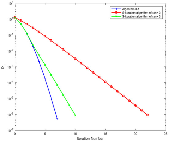
In order to show the effectiveness of our Algorithm 3, we compare it to two others algorithms: S-iteration algorithm of rank 2 (7) and S-iteration algorithm of rank 3 (8). In Algorithm 3, we set $a_n=b_n=c_n=0.5+\frac{1}{n+2}$. In S-iteration algorithm of rank 2 and S-iteration algorithm of rank 3, we take $a_n=b_n=c_n=0.5-\frac{1}{n+2}$. Let $x^{*}=(0,0,0,1)$ and a random initial point

$$x_0=(0.69445440978475,1.01382609280137,0.99360871330745,1.87012527625153).$$

We denoted $D_n=d(x_n,x^{*})<{10}^{-6}$ as the stopping criterion. The computational results of Algorithm 3, S-iteration algorithm of rank 2 and S-iteration algorithm of rank 3 are indicated in Table 2 and Figure 2 for the behavior of $D_n$. It is seen that our proposed method converges faster than other iterative methods.

Table 2. Numerical experiments of Example 2.

Algorithm	Iteration	Time (s)
Algorithm 3	7	0.0064
S-iteration algorithm of rank 2	22	0.0188
S-iteration algorithm of rank 3	10	0.0198

Figure 2. Numerical behavior of $\left\{D_n\right\}$ for Example 2.

5. Applications

5.1. Inclusion Problems

Let $\Psi \left(M\right)$ be the set of all multivalued vector fields $A:M\to 2^{TM}$ such that $A\left(x\right)\in T_{x}M,$ $\forall x\in M$, and denote $D\left(A\right)$ the domain of A defined by $D\left(A\right)=\{x\in M:A(x)\ne \varnothing \}$. Suppose that $A\in \Psi \left(M\right)$ is a multivalued vector. A point $x^{*}\in M$ is called a singularity of A such that $\mathbf{0}\in A\left(x^{*}\right)$. The set of all singularities of A is assigned by $A^{-1}\left(\mathbf{0}\right)=\{x\in C:\mathbf{0}\in A\left(x\right)\}.$

Next, we recall concept of monotonicity for a multivalued vector field on Hadamard manifolds.

Definition 2 

([38]).A vector field $A\in \Psi \left(M\right)$ is said to be

(i)

monotone if $\forall x,y\in D\left(A\right)$

$$⟨u,{exp}_x^{-1}y⟩\le ⟨v,-{exp}_y^{-1}x⟩,\forall u\in A\left(x\right),v\in A\left(y\right);$$

and

(ii)

maximal monotone if it is monotone and $\forall x\in M$ and $u\in T_{x}M$, the condition

$$⟨u,{exp}_x^{-1}y⟩\le ⟨v,-{exp}_y^{-1}x⟩,\forall y\in D\left(A\right),v\in A\left(y\right)⟹u\in A\left(x\right).$$

Li et al. [21] provided a definition for the resolvent of a multivalued vector field as well as a firmly nonexpansive mapping on Hadamard manifolds.

Definition 3 

([21]).Given $\lambda >0$ and let the multivalued vector field $A\in \Psi \left(M\right)$, the resolvent related to A of order λ is a multivalued map $J_{\lambda }^A:M\to 2^M$ defined by

$$J_{\lambda }^A\left(x\right):=\left\{y\in M:\frac{{exp}_y^{-1}x}{\lambda }\in A\left(y\right)\right\},\forall x\in M.$$

Remark 2 

([21]).Assume that $\lambda >0.$ According to the definition of the resolvent, then the range of the resolvent $J_{\lambda }^A$ is contained the domain of A and $\mathcal{F}\left(J_{\lambda }^A\right)=A^{-1}\left(\mathbf{0}\right).$

Definition 4 

([21]).A mapping $T:M\to M$ is said to be firmly nonexpansive if for any two points $x,y\in M$, the function $\gamma :[0,1]\to [0,+\infty )$ defined by

$$\gamma \left(t\right):=d({exp}_{x}t{exp}_x^{-1}Tx,{exp}_{y}t{exp}_y^{-1}Ty),\forall t\in [0,1],$$

is nonincreasing.

According to the concept of firmly nonexpansive mappings, it is straightforward to deduce that all firmly nonexpansive mappings are nonexpansive. By the way, the monotonicity and the expansiveness are closely related to one another.

Theorem 2 

([21]).Let a vector field $A\in \Psi \left(M\right)$. Then, the multivalued vector field A is monotone ⟺$J_{\lambda }^A$ is single-valued and firmly nonexpansive, $\forall \lambda >0$.

Let $g:M\to \mathbb{R}\cup \{+\infty \}$ be a geodesic convex function. We know that the subdifferential $\partial g\left(x\right)$ at x is closed and geodesic convex [33] and is defined as

$$\partial g\left(x\right)=\{u\in T_{x}M:g\left(y\right)\ge g\left(x\right)+⟨u,{exp}_x^{-1}y⟩,\forall y\in M\}.$$

(31)

The following lemma states that the subdifferential $\partial g$ is maximal monotone vector field.

Lemma 4 

([39]).Let $g:M\to \mathbb{R}\cup \{+\infty \}$ be a proper lower semicontinuous geodesic convex function and $D\left(g\right)=M.$ Then, the subdifferential $\partial g$ of g is a maximal monotone vector field.

Clearly,

$$x\in \underset{M}{min}g⟺\mathbf{0}\in \partial g\left(x\right),$$

where $\underset{M}{min}g=\{x\in M:g\left(x\right)\le g\left(y\right),\forall y\in M\}$ stands for the set of minimizers.

Here we consider an inclusion problem in the setting of Hadamard manifolds. Then the problem is to find $x^{*}\in M$ such that

$$x^{*}\in A^{-1}\left(\mathbf{0}\right)\cap B^{-1}\left(\mathbf{0}\right),$$

(32)

where $A,B\in \Psi \left(M\right)$. $\mathbb{S}$ represents the solution set of the inclusion problem (32). In light of Remark 2, the challenge of finding singularities of A is transformed into the problem of finding fixed points of the mapping $J_{\lambda }^A$.

Next, we apply Algorithm 3 to find a common singularity of two multivalued monotone vector fields.

Theorem 3. 

Let $A,B\in \Psi \left(M\right)$ be multivalued monotone vector fields such that $\mathbb{S}\ne \varnothing$. Assume that $\left\{a_n\right\},$ $\left\{b_n\right\}$ and $\left\{c_n\right\}$ are real positive sequences satisfying $0<k_1\le a_n\le \widehat{k_1}<1,0<k_2\le b_n\le \widehat{k_2}<1$ and $0<k_3\le c_n\le \widehat{k_3}<1,$ $\forall n\in \mathbb{N}$. Let $x_0\in M$ and $\left\{x_n\right\}$ is defined by

$$\left\{\begin{array}{c}{z}_n={exp}_{x_n}{c}_n{exp}_{x_n}^{-1}{J}_{\lambda }^A\left(x_n\right),\hfill \\ y_n={exp}_{z_n}{b}_n{exp}_{z_n}^{-1}{J}_{\mu }^B\left(z_n\right),\hfill \\ x_{n+1}={exp}_{J_{\lambda }^A\left(z_n\right)}{a}_n{exp}_{J_{\lambda }^A\left(z_n\right)}^{-1}{J}_{\mu }^B\left(y_n\right),\forall n\in \mathbb{N},\hfill \end{array}\right.$$

(33)

where $\lambda ,\mu >0$. Then, $\left\{x_n\right\}$ converges to an element in $A^{-1}\left(\mathbf{0}\right)\cap B^{-1}\left(\mathbf{0}\right).$

Proof. 

Set $g=J_{\lambda }^A$ and $h=J_{\mu }^B$. Form Theorem 2, g and h are single-valued and firmly nonexpansive mappings. Hence, they are nonexpansive mappings with $\mathcal{F}\left(g\right)=A^{-1}\left(\mathbf{0}\right)$ and $\mathcal{F}\left(h\right)=B^{-1}\left(\mathbf{0}\right)$. From the hypothesis, $\mathcal{F}\left(g\right)\cap \mathcal{F}\left(h\right)=A^{-1}\left(\mathbf{0}\right)\cap B^{-1}\left(\mathbf{0}\right)\ne \varnothing .$ Therefore, according to Theorem 1, we get the desired result. □

Now, we discuss a numerical experiment which support Theorem 3.

Example 3. 

Let $M:={\mathbb{R}}_{++}^m=\{x\in {\mathbb{R}}^m:x_i>0,i=1,\dots ,m\}$ and ${\mathbb{R}}_{+}^m=\{x\in {\mathbb{R}}^m:x_i\ge 0,i=1,\dots ,m\}$. As [28], let $({\mathbb{R}}_{++}^m,⟨·,·⟩)$ be the Riemannian manifold with the Riemannian metric $⟨·,·⟩$ defined by $⟨u,v⟩:=u^{T}W\left(x\right)v,$ $\forall x\in {\mathbb{R}}_{++}^m$ and $u,v\in T_x{\mathbb{R}}_{++}^m$, where $W\left(x\right)$ is a diagonal metrix defined by $W\left(x\right)=\mathrm{diag}\left(x_1^{-2},x_2^{-2},\dots ,x_m^{-2}\right).$ Tangent space at $x\in {\mathbb{R}}_{++}^m$, denoted by $T_x{\mathbb{R}}_{++}^m$. The Riemannian distance $d:{\mathbb{R}}_{++}^m\times {\mathbb{R}}_{++}^m\to {\mathbb{R}}_{+}^m$ is defined by

$$d(x,y):=\sqrt{\sum _{i=1}^m{ln}^2\frac{x_i}{y_i}},\forall x,y\in {\mathbb{R}}_{++}^m.$$

Thus, $({\mathbb{R}}_{++}^m,⟨·,·⟩)$ is a Hadamard manifold. The exponential map on ${\mathbb{R}}_{++}^m$ is given by

$${exp}_{x}tv=\left(x_1{e}^{\frac{v_{1}t}{x_1}},x_2{e}^{\frac{v_{2}t}{x_2}},\dots ,x_m{e}^{\frac{v_{m}t}{x_m}}\right),$$

for $x\in {\mathbb{R}}_{++}^m$ and $\upsilon \in T_x{\mathbb{R}}_{++}^m.$ The inverse of the exponential map is assigned by

$${exp}_x^{-1}y=\left(x_{1}ln\frac{y_1}{x_1},x_{2}ln\frac{y_2}{x_2},\dots ,x_{m}ln\frac{y_m}{x_m}\right),\forall x,y\in {\mathbb{R}}_{++}^m.$$

Let $g:{\mathbb{R}}_{++}^m\to \mathbb{R}$ be a mapping defined by

$$g\left(x\right):=\sum _{i=1}^m{g}_i\left(x_i\right),g_i\left(x_i\right):={\alpha }_{i}ln\left(x_i^{{\omega }_i}+{\beta }_i\right)-{\rho }_{i}ln\left(x_i\right),i=1,\dots ,m,$$

where ${\alpha }_i,{\beta }_i,{\rho }_i,{\omega }_i\in {\mathbb{R}}_{++}$ satisfy ${\rho }_i<{\alpha }_i{\omega }_i$ and ${\omega }_i\ge 2$ for $i=1,\dots ,m$. The minimizer of g is $x^{*}=(x_1^{*},x_2^{*},\dots ,x_m^{*})$, where $x_i^{*}=\sqrt[{\omega }_i]{{\beta }_i{\rho }_i/({\alpha }_i{\omega }_i-{\rho }_i)},$ for $i=1,\dots ,m$. Ferreira et al. [19] showed that g is a geodesic convex function in $({\mathbb{R}}_{++}^m,⟨·,·⟩)$. Taking ${\alpha }_i={\beta }_i={\rho }_i=1$ and ${\omega }_i=2$, for $i=1,\dots ,m$, we obtain 1 as the minimizer of the mapping g. Let $h:{\mathbb{R}}_{++}^m\to \mathbb{R}$ be a mapping defined by

$$h\left(x\right):=d(1,x),\forall x\in {\mathbb{R}}_{++}^m.$$

It is easy to see that h is geodesic convex function, and 1 is the minimizer.

From (31), we have

$$\partial g\left(x\right)=\left\{u\in T_x{\mathbb{R}}_{++}^m|g\left(y\right)\ge g\left(x\right)+\frac{u}{x}ln\left(\frac{x}{y}\right)\right\},\forall y\in {\mathbb{R}}_{++}^m,$$

and

$$\partial h\left(x\right)=\left\{u\in T_x{\mathbb{R}}_{++}^m|d(1,y)\ge d(1,x)+\frac{u}{x}ln\left(\frac{x}{y}\right)\right\},\forall y\in {\mathbb{R}}_{++}^m.$$

The subdifferential $\partial g$ and $\partial h$ are maxiaml monotone vector fields, as shown by Lemma 4. Thus, we instead the multivalued monotone vector fields A and B by $\partial g$ and $\partial h$, respectively. In addition to it, we have

$$J_{\lambda }^{\partial g}\left(x\right)=\underset{y\in {\mathbb{R}}_{++}^m}{argmin}\left\{g\left(y\right)+\frac{1}{2\lambda }{d}^2(y,x)\right\},\forall \lambda >0,$$

and

$$J_{\mu }^{\partial h}\left(x\right)=\underset{y\in {\mathbb{R}}_{++}^m}{argmin}\left\{d(1,y)+\frac{1}{2\mu }{d}^2(y,x)\right\},\forall \mu >0.$$

Due to the fact that the minimizer of both g and h is 1, it is possible for us to observe that $\mathbb{S}:=A^{-1}\left(\mathbf{0}\right)\cap B^{-1}\left(\mathbf{0}\right)=\left\{1\right\}$.

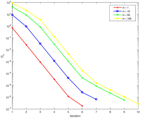
Choose $a_n=b_n=c_n=0.5$, $\lambda =\mu =1$, and let $x^{*}=1$. We take into account of the various of numbers for dimension m. Denoted $D_n=d{(x_n,x^{*})}^2<{10}^{-6}$ as the stopping criterion. The initial values $x_0$ are randomly generated in MATLAB. Both Table 3 and Figure 3 include the numerical results that we obtained.

Table 3. Numerical experiments of Example 3.

${\mathit{D}}_{\mathit{n}}$	Dimension
	$\mathit{m}=\mathbf{1}$	$\mathit{m}=\mathbf{10}$	$\mathit{m}=\mathbf{50}$	$\mathit{m}=\mathbf{100}$
$D_1$	0.975719	8.397434	40.647008	86.538043
$D_2$	0.036959	0.834326	8.445068	21.070651
$D_3$	0.001303	0.029538	0.794156	3.402976
$D_4$	4.582065 × ${10}^{-5}$	0.001043	0.027961	0.129793
$D_5$	1.641608 × ${10}^{-6}$	3.782427 × ${10}^{-5}$	0.000991	0.004588
$D_6$	2.488131 × ${10}^{-7}$	2.415600 × ${10}^{-6}$	4.070337 × ${10}^{-5}$	0.000176
$D_7$	-	6.194778 × ${10}^{-7}$	8.331605 × ${10}^{-6}$	1.623930 × ${10}^{-5}$
$D_8$	-	-	2.111748 × ${10}^{-6}$	4.140798 × ${10}^{-6}$
$D_9$	-	-	5.425004 × ${10}^{-7}$	1.076243 × ${10}^{-6}$
$D_{10}$	-	-	-	2.742307 × ${10}^{-7}$

Figure 3. Numerical behavior of $\left\{D_n\right\}$ for Example 3.

Remark 3. 

(i) 

Numerical experiments, as shown in Table 3, demonstrate that the proposed Algorithm (33) with different dimensional sizes converges to a common singularity of maximal monotone multivalued vector fields. Our method is efficient and simple to implement for solving the inclusion problem (32). Furthermore, the number of iterations required by Algorithm (33) is unaffected by the dimension selection; in fact, the number of iterations required by the proposed method is only slightly affected by the dimension leaping change.

(ii) 

The functions g and h in the Example 3 are nonconvex functions in the Euclidean sense. Therefore, the iterative method [12] can’t be applied to solve the problem (32).

5.2. Convex Feasibility Problems

Suppose that C is a nonempty, closed and geodesic convex subset of M. The projection operator $P_C(·):M\to C$ is defined by $P_C\left(x\right):=\{z:d(x,z)\le d(x,y),\forall y\in C\},$ $\forall x\in M$. We know that the projection operator $P_C$ is single-valued and firmly nonexpansive [21].

Let $C_1$ and $C_2$ are nonempty, closed and geodesic convex subsets of M such that $C_1\cap C_2=\varnothing$. Since $P_{C_1}:M\to C_1$ with $\mathcal{F}\left(P_{C_1}\right)=C_1$ and $P_{C_2}:M\to C_2$ with $\mathcal{F}\left(P_{C_2}\right)=C_2$ are nonexpansive mappings. Therefore, $\mathsf{\Gamma }(P_{C_1},P_{C_2})=C_1\cap C_2$. This means that finding an element in $\mathsf{\Gamma }(P_{C_1},P_{C_2})$ is analogous to finding a point in the intersection of two nonempty, closed and geodesic convex subsets of Hadamard manifolds.

Next, we apply Algorithm 3 to find a point in the intersection of two nonempty, closed, and geodesic convex subsets of Hadamard manifolds.

Theorem 4. 

Let $C_1$ and $C_2$ are nonempty, closed, and geodesic convex subset of M such that $C_1\cap C_2\ne \varnothing$. Assume that $\left\{a_n\right\},$ $\left\{b_n\right\}$ and $\left\{c_n\right\}$ are real positive sequences satisfying $0<k_1\le a_n\le \widehat{k_1}<1,0<k_2\le b_n\le \widehat{k_2}<1$ and $0<k_3\le c_n\le \widehat{k_3}<1,$ $\forall n\in \mathbb{N}$. Let $x_0\in M$ and $\left\{x_n\right\}$ is defined by

$$\left\{\begin{array}{c}{z}_n={exp}_{x_n}{c}_n{exp}_{x_n}^{-1}{P}_{C_1}\left(x_n\right),\hfill \\ y_n={exp}_{z_n}{b}_n{exp}_{z_n}^{-1}{P}_{C_2}\left(z_n\right),\hfill \\ x_{n+1}={exp}_{P_{C_1}\left(z_n\right)}{a}_n{exp}_{P_{C_1}\left(z_n\right)}^{-1}{P}_{C_2}\left(y_n\right),\forall n\in \mathbb{N}.\hfill \end{array}\right.$$

(34)

Then, $\left\{x_n\right\}$ converges to an element in $C_1\cap C_2.$

Proof. 

Set $g=P_{C_1}$ and $h=P_{C_2}$. Then, g and h are nonexpansive mappings with $\mathcal{F}\left(g\right)=C_1$ and $\mathcal{F}\left(h\right)=C_2$. From the hypothesis, $\mathcal{F}\left(g\right)\cap \mathcal{F}\left(h\right)=C_1\cap C_2\ne \varnothing .$ Therefore, according to Theorem 1, we get the desired result. □

Now, we discuss a numerical experiment which support Theorem 4.

Example 4. 

Let $M:=\mathbb{H}=\{(t_1,t_2)\in {\mathbb{R}}^2|t_2>0\}$ be the Poincaré plane endowed with the Riemannian metric defined by

$$g_{11}=g_{22}:=\frac{1}{t_2^2},g_{12}:=0,\forall (t_1,t_2)\in \mathbb{H}.$$

(35)

The sectional curvature of $\mathbb{H}$ is equal to $-1$, and the geodesics of the Poincaré plane are the semilines ${\phi }_a:t_1=a,t_2>0$ and the semicircles ${\phi }_{b,r}:{(t_1-b)}^2+t_2^2=r^2,t_2>0;$ or admit the following natural parameterizations:

$$\begin{array}{c}{\phi }_a:t_1=a,t_2=e^s,s\in (-\infty ,+\infty );\hfill \\ {\phi }_{b,r}:t_1=-rtanhs,t_2={\displaystyle \frac{r}{coshs}},s\in (-\infty ,+\infty );\hfill \end{array}$$

(36)

see e.g., [33]. Furthermore, consider two points $y=(t_1^y,t_2^y)$ and $z=(t_1^z,t_2^z)$ in $\mathbb{H}$. Then, the Riemannian distance between y and z is defined by

$$d_{\mathbb{H}}(y,z)=\left\{\begin{array}{c}\left|ln{\displaystyle \frac{t_2^z}{t_2^y}}\right|,\mathrm{if}{t}_1^y=t_1^z,\hfill \\ \left|ln{\displaystyle \frac{t_1^y-b+r}{t_1^z-b+r}}·{\displaystyle \frac{t_2^z}{t_2^y}}\right|,\mathrm{if}{t}_1^y\ne t_1^z,\hfill \end{array}\right.$$

where

$$b={\displaystyle \frac{{\left(t_1^y\right)}^2+{\left(t_2^y\right)}^2-({\left(t_1^z\right)}^2+{\left(t_2^z\right)}^2)}{2(t_1^y-t_1^z)}}\mathrm{and}r=\sqrt{{(t_1^y-b)}^2+{\left(t_2^y\right)}^2}.$$

To get the expression of ${exp}_y^{-1}z$, we consider a smooth geodesic curve φ joining y to z defined by

$$\phi \left(s\right):=({\phi }_1\left(s\right),{\phi }_2\left(s\right)),\forall s\in [0,1],$$

where ${\phi }_1\left(s\right)$ and ${\phi }_2\left(s\right)$ are respectively defined by

$${\phi }_1\left(s\right):=\left\{\begin{array}{cc}{t}_1^y\hfill & \mathrm{if}{t}_1^y=t_1^z,\hfill \\ b-rtanh\left((1-s)·\mathrm{arctanh}{\displaystyle \frac{b-t_1^y}{r}}+s·\mathrm{arctanh}{\displaystyle \frac{b-t_1^z}{r}}\right),\hfill & \mathrm{if}{t}_1^y\ne t_1^z,\hfill \end{array}\right.$$

and

$${\phi }_2\left(s\right):=\left\{\begin{array}{cc}{e}^{(1-s)·ln{t}_2^y+s·ln{t}_2^z}\hfill & \mathrm{if}{t}_1^y=t_1^z,\hfill \\ {\displaystyle \frac{r}{cosh\left((1-s)·\mathrm{arctanh}{\displaystyle \frac{b-t_1^y}{r}}+s·\mathrm{arctanh}{\displaystyle \frac{b-t_1^z}{r}}\right)}},\hfill & \mathrm{if}{t}_1^y\ne t_1^z.\hfill \end{array}\right.$$

By the Riemannian metric endowed on $\mathbb{H}$ (c.f. (35)), one checks that

$${\phi }^{{}^{\prime }}\left(0\right)={\left.\left({\displaystyle \frac{\mathrm{d}{\phi }_1\left(s\right)}{\mathrm{d}s}},{\displaystyle \frac{\mathrm{d}{\phi }_2\left(s\right)}{\mathrm{d}s}}\right)\right|}_{s=0};$$

see [32] (p. 7). Therefore, by elementary calculus, we get

$${exp}_y^{-1}z={\phi }^{{}^{\prime }}\left(0\right)=\left\{\begin{array}{cc}\left(0,t_2^{y}ln{\displaystyle \frac{t_2^z}{t_2^y}}\right),\hfill & \mathrm{if}{t}_1^y=t_1^z,\hfill \\ {\displaystyle \frac{t_2^y\left(\mathrm{arctanh}{\displaystyle \frac{b-t_1^y}{r}}-\mathrm{arctanh}{\displaystyle \frac{b-t_1^z}{r}}\right)}{r}}(t_2^y,b-t_1^y),\hfill & \mathrm{if}{t}_1^y\ne t_1^z.\hfill \end{array}\right.$$

(37)

It follows from [40] [Example 5.1], that we must let $C_1,C_2$ be closed convex subsets of $\mathbb{H}$ defined as

$$C_1:=\{(t_1,t_2)\in \mathbb{H}:t_2\ge 1\},$$

and

$$C_2:=\{(t_1,t_2)\in \mathbb{H}:t_1^2+t_2^2\le 1)\}.$$

From [33] (p. 301), $C_1$ and $C_2$ are convex because that $C_1$ is level set convex function $f:\mathbb{H}\to \mathbb{R}$ defined by

$$f\left(y\right)=\frac{1}{t_2},\forall y=(t_1,t_2)\in \mathbb{H}$$

and $\phi :=\{(t_1,t_2)\in M:t_1+t_2=1\}$ is a geodesic of $\mathbb{H}$, receptively. Moreover $\mathsf{\Gamma }(P_{C_1},P_{C_2})=\left\{(0,1)\right\}$,

$$P_{C_1}\left(x\right)=(t_1,1),\forall x=(t_1,t_2)\notin C_1,$$

and

$$P_{C_2}\left(x\right)=\left({\displaystyle \frac{2t_1}{t_1^2+t_2^2+1}},\sqrt{1-{\left({\displaystyle \frac{2t_1}{t_1^2+t_2^2+1}}\right)}^2}\right),\forall x=(t_1,t_2)\notin C_2.$$

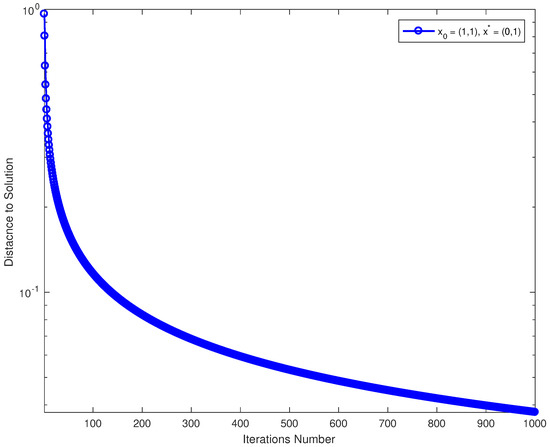
Choose $a_n=b_n=c_n=0.7+\frac{1}{n+3}$ and the initial point $x_0=(1,1)$ with $x^{*}=(0,1)$. The computational results of Algorithm (34) are presented in Table 4 and Figure 4.

Table 4. The numerical results of Algorithm (34).

Iteration	Algorithm (34)
	${\mathit{x}}_{\mathit{n}}$	$\mathit{d}({\mathit{x}}_{\mathit{n}},{\mathit{x}}^{\mathbf{*}})$
0	(1,1)	0.962424
1	(0.666667,0.745356)	0.804719
2	(0.558497,0.829507)	0.630646
3	(0.493526,0.869731)	0.540711
4	(0.448527,0.893769)	0.482855
5	(0.414798,0.909914)	0.441392
6	(0.388202,0.921574)	0.409681
7	(0.366477,0.930427)	0.384347
8	(0.348263,0.937397)	0.363465
9	(0.332683,0.943039)	0.345842
10	(0.319143,0.947707)	0.330693
⋮	⋮	⋮
50	(0.159591,0.987183)	0.160967
⋮	⋮	⋮
100	(0.115512,0.993306)	0.116031
⋮	⋮	⋮
500	(0.052958,0.998597)	0.053007
⋮	⋮	⋮
1000	(0.037602,0.999293)	0.037619

Figure 4. Distance to solution $x^{*}=(0,1)$ of each iteration number where the initial point is $x_0=(1,1)$.

6. Conclusions

The problem of finding common fixed points of two nonexpansive mappings in the setting Hadamard manifolds is the subject of this research. Regarding the solution to this problem, a new three-step method is suggested. The proposed method has been shown to converge under certain assumptions. The effectiveness of the proposed method is shown by numerical examples.

References

- Bauschke, H.H.; Combettes, P.L. Convex Analysis and Monotone Operator Theory in Hilbert Spaces, 2nd ed.; CMS Books in Mathematics/Ouvrages de Mathématiques de la SMC; Springer: Cham, Switzerland, 2017; p. xix+619, With a foreword by Hédy Attouch. [Google Scholar] [CrossRef]
- Bauschke, H.H.; Borwein, J.M. On projection algorithms for solving convex feasibility problems. SIAM Rev. 1996, 38, 367–426. [Google Scholar] [CrossRef]
- Kitkuan, D.; Kumam, P.; Martínez-Moreno, J. Generalized Halpern-type forward-backward splitting methods for convex minimization problems with application to image restoration problems. Optimization 2020, 69, 1557–1581. [Google Scholar] [CrossRef]
- Padcharoen, A.; Kumam, P.; Cho, Y.J. Split common fixed point problems for demicontractive operators. Numer. Algorithms 2019, 82, 297–320. [Google Scholar] [CrossRef]
- Picard, E. Mémoire sur la théorie des équations aux dérivées partielles et la méthode des approximations successives. Journal de Mathématiques Pures et Appliquées 1890, 6, 145–210. [Google Scholar]
- Mann, W.R. Mean value methods in iteration. Proc. Am. Math. Soc. 1953, 4, 506–510. [Google Scholar] [CrossRef]
- Ishikawa, S. Fixed points by a new iteration method. Proc. Am. Math. Soc. 1974, 44, 147–150. [Google Scholar] [CrossRef]
- Agarwal, R.P.; O’Regan, D.; Sahu, D.R. Iterative construction of fixed points of nearly asymptotically nonexpansive mappings. J. Nonlinear Convex Anal. 2007, 8, 61–79. [Google Scholar]
- Sahu, V.K.; Pathak, H.K.; Tiwari, R. Convergence theorems for new iteration scheme and comparison results. Aligarh Bull. Math. 2016, 35, 18–42. [Google Scholar]
- Thakur, B.S.; Thakur, D.; Postolache, M. A new iteration scheme for approximating fixed points of nonexpansive mappings. Filomat 2016, 30, 2711–2720. [Google Scholar] [CrossRef]
- Li, C.; López, G.; Martín-Márquez, V. Iterative algorithms for nonexpansive mappings on Hadamard manifolds. Taiwan. J. Math. 2010, 14, 541–559. [Google Scholar] [CrossRef]
- Padcharoen, A.; Sukprasert, P. Nonlinear Operators as Concerns Convex Programming and Applied to Signal Processing. Mathematics 2019, 7, 866. [Google Scholar] [CrossRef]
- Sahu, D.R.; Babu, F.; Sharma, S. The S-iterative techniques on Hadamard manifolds and applications. J. Appl. Numer. Optim. 2020, 2, 353–371. [Google Scholar] [CrossRef]
- Debnath, P.; Konwar, N.; Radenović, S. (Eds.) Metric Fixed Point Theory. Applications in Science, Engineering and Behavioural Sciences; Forum for Interdisciplinary Mathematics (FFIM); Springer: Singapore, 2021. [Google Scholar] [CrossRef]
- Todorčević, V. Harmonic Quasiconformal Mappings and Hyperbolic Type Metrics; Springer: Cham, Switzerland, 2019. [Google Scholar] [CrossRef]
- Khuri, S.A.; Louhichi, I. A novel Ishikawa-Green’s fixed point scheme for the solution of BVPs. Appl. Math. Lett. 2018, 82, 50–57. [Google Scholar] [CrossRef]
- Sintunavarat, W.; Pitea, A. On a new iteration scheme for numerical reckoning fixed points of Berinde mappings with convergence analysis. J. Nonlinear Sci. Appl. 2016, 9, 2553–2562. [Google Scholar] [CrossRef]
- Ali, J.; Ali, F.; Kumar, P. Approximation of fixed points for Suzuki’s generalized non-expansive mappings. Mathematics 2019, 7, 522. [Google Scholar] [CrossRef]
- Ferreira, O.P.; Louzeiro, M.S.; Prudente, L.F. Gradient method for optimization on Riemannian manifolds with lower bounded curvature. SIAM J. Optim. 2019, 29, 2517–2541. [Google Scholar] [CrossRef]
- Ferreira, O.P.; Oliveira, P.R. Proximal point algorithm on Riemannian manifolds. Optimization 2002, 51, 257–270. [Google Scholar] [CrossRef]
- Li, C.; López, G.; Martín-Márquez, V.; Wang, J.H. Resolvents of set-valued monotone vector fields in Hadamard manifolds. Set-Valued Var. Anal. 2011, 19, 361–383. [Google Scholar] [CrossRef]
- Németh, S.Z. Variational inequalities on Hadamard manifolds. Nonlinear Anal. 2003, 52, 1491–1498. [Google Scholar] [CrossRef]
- Salisu, S.; Kumam, P.; Sriwongsa, S.; Abubakar, J. On minimization and fixed point problems in Hadamard spaces. Comput. Appl. Math. 2022, 41, 22. [Google Scholar] [CrossRef]
- Kumam, P.; Chaipunya, P. Equilibrium problems and proximal algorithms in Hadamard spaces. J. Nonlinear Anal. Optim. 2017, 8, 155–172. [Google Scholar]
- Kirk, W.; Shahzad, N. Fixed Point Theory in Distance Spaces; Springer: Cham, Switzerland, 2014; p. xii+173. [Google Scholar] [CrossRef]
- Salisu, S.; Minjibir, M.S.; Kumam, P.; Sriwongsa, S. Convergence theorems for fixed points in CAT_p(0) spaces. J. Appl. Math. Comput. 2022, 1–20. [Google Scholar] [CrossRef]
- Adler, R.L.; Dedieu, J.P.; Margulies, J.Y.; Martens, M.; Shub, M. Newton’s method on Riemannian manifolds and a geometric model for the human spine. IMA J. Numer. Anal. 2002, 22, 359–390. [Google Scholar] [CrossRef]
- Da Cruz Neto, J.X.; Ferreira, O.P.; Pérez, L.R.L.; Németh, S.Z. Convex- and monotone-transformable mathematical programming problems and a proximal-like point method. J. Glob. Optim. 2006, 35, 53–69. [Google Scholar] [CrossRef]
- Grohs, P.; Hosseini, S. Nonsmooth trust region algorithms for locally Lipschitz functions on Riemannian manifolds. IMA J. Numer. Anal. 2016, 36, 1167–1192. [Google Scholar] [CrossRef]
- Kristály, A. Nash-type equilibria on Riemannian manifolds: A variational approach. J. Math. Pures Appl. 2014, 101, 660–688. [Google Scholar] [CrossRef]
- Sakai, T. Riemannian Geometry. In Translations of Mathematical Monographs; American Mathematical Society: Providence, RI, USA, 1996; Volume 149, p. xiv+358, Translated from the 1992 Japanese original by the author. [Google Scholar]
- do Carmo, M.P.A. Riemannian geometry. In Mathematics: Theory & Applications; Birkhauser Boston, Inc.: Boston, MA, USA, 1992; p. xiv+300, Translated from the second Portuguese edition by Francis Flaherty. [Google Scholar] [CrossRef]
- Udrişte, C. Convex Functions and Optimization Methods on Riemannians Manifolds. In Mathematics and Its Applications; Kluwer Academic Publishers Group: Dordrecht, the Netherlands, 1994; Volume 297, p. xviii+348. [Google Scholar] [CrossRef]
- Bridson, M.R.; Haefliger, A. Metric spaces of non-positive curvature. In Grundlehren der Mathematischen Wissenschaften [Fundamental Principles of Mathematical Sciences]; Springer: Berlin/Heidelberg, Germany, 1999; Volume 319, p. xxii+643. [Google Scholar] [CrossRef]
- Al-Homidan, S.; Ansari, Q.H.; Babu, F.; Yao, J.C. Viscosity method with a ϕ-contraction mapping for hierarchical variational inequalities on Hadamard manifolds. Fixed Point Theory 2020, 21, 561–584. [Google Scholar] [CrossRef]
- Ferreira, O.P.; Pérez, L.R.L.; Németh, S.Z. Singularities of monotone vector fields and an extragradient-type algorithm. J. Glob. Optim. 2005, 31, 133–151. [Google Scholar] [CrossRef]
- Tang, G.J.; Huang, N.J. Korpelevich’s method for variational inequality problems on Hadamard manifolds. J. Glob. Optim. 2012, 54, 493–509. [Google Scholar] [CrossRef]
- da Cruz Neto, J.X.; Ferreira, O.P.; Lucambio Pérez, L.R. Monotone point-to-set vector fields. Balkan J. Geom. Appl. 2000, 5, 69–79, Dedicated to Professor Constantin Udrişte. [Google Scholar]
- Li, C.; López, G.; Martín-Márquez, V. Monotone vector fields and the proximal point algorithm on Hadamard manifolds. J. Lond. Math. Soc. 2009, 79, 663–683. [Google Scholar] [CrossRef]
- Wang, X.; Li, C.; Yao, J.C. Projection algorithms for convex feasibility problems on Hadamard manifolds. J. Nonlinear Convex Anal. 2016, 17, 483–497. [Google Scholar]
Publisher’s Note: MDPI stays neutral with regard to jurisdictional claims in published maps and institutional affiliations. |
© 2022 by the authors. Licensee MDPI, Basel, Switzerland. This article is an open access article distributed under the terms and conditions of the Creative Commons Attribution (CC BY) license (https://creativecommons.org/licenses/by/4.0/).