Dynamical Analysis of Discrete-Time Two-Predators One-Prey Lotka–Volterra Model

Abstract

This research manifesto has a comprehensive discussion of the global dynamics of an achievable discrete-time two predators and one prey Lotka–Volterra model in three dimensions, i.e., in the space $R^3$. In some assertive parametric circumstances, the discrete-time model has eight equilibrium points among which one is a special or unique positive equilibrium point. We have also investigated the local and global behavior of equilibrium points of an achievable three-dimensional discrete-time two predators and one prey Lotka–Volterra model. The conversion of a continuous-type model into its discrete counterpart model has been completed by adopting a dynamically consistent nonstandard difference scheme with the end goal that the equilibrium points are conserved in twin cases. The difficulty lies in how to find all fixed points $O,P,Q,R,S,T,U,V$ and the Jacobian matrix and its characteristic polynomial at the unique positive fixed point. For that purpose, we use Mathematica software to find the equilibrium points and all of the Jacobian matrices at those equilibrium points. Moreover, we discuss boundedness conditions for every solution and prove the existence of a unique positive equilibrium point. We discuss the local stability of the obtained system about all of its equilibrium points. The discrete Lotka–Volterra model in three dimensions is given by system (3), where parameters $\alpha ,\beta ,\gamma ,\delta ,\zeta ,\eta ,\mu ,\epsilon ,\upsilon ,\rho ,\sigma ,\omega \in {\mathbb{R}}^{+}$ and initial conditions $x_0,y_0,z_0$ are positive real numbers. Additionally, the rate of convergence of a solution that converges to a unique positive equilibrium point is discussed. To represent theoretical perceptions, some numerical debates are introduced, including phase portraits.

1. Introduction

The present research article has a detailed discussion on the global behavior of a possible three-dimensional Lotka–Volterra model in discrete form. Discrete Lotka–Volterra models have many applications in applied sciences. As an example, mathematical biology was the first field to utilize models, and then, other fields followed [1,2,3,4]. Various variations of the Lotka–Volterra predator–prey model have been proposed that provide more realistic descriptions of population interactions. There may be considerations, which led to the development of the logistic equation if the rabbit population is always higher than the fox population. A sufficient number of rabbits may interfere with each other’s quest for food and space if they become too numerous. A more complicated system can be used to describe this effect mathematically.

An important role is played by ordinary differential equations when it comes to analyzing the dynamics of real-life situations such as cell signaling pathways, population growth, and enzymatic inhibitor reactions. Although differential equations are an excellent tool for understanding the dynamic behavior of such systems, most biological models have memory or aftereffects. Often, such effects are overlooked in systems. Fractional-order differential equations play an important role in understanding and identifying these effects. The idea of fractional differential equations and their applications in nonlinear biochemical reaction models has been studied in [5,6].

A discrete dynamical system may be a suitable alternative model if foxes can survive on an alternative resource, although rabbits are their natural prey. Discrete-time models described by difference equations are well known to be more suitable than continuous-time models [7,8,9,10,11,12]. There is a great deal of importance in applications for nonlinear difference equations of order greater than one. In biology, ecology, physiology, physics, engineering, and economics, such equations naturally appear as discrete analogs and numerical solutions of differential and delay differential equations. Rational difference equations are special cases of nonlinear dynamical systems. For a basic understanding of difference equations and rational difference equations, see [13,14]. Recently, many authors have discussed the dynamics of rational difference equations [2,15]. J. Alebraheem and Y. Abu-Hasan [16] examined the dynamical associations of a three-animal type evolved way of life model, where two predators are competing for one prey. The rates of growth of two predators and one prey are depicted by a law of logistics in which the carrying capacity of predators relies upon an accessible measure of prey. The functional response Holling type-$II$ is utilized to portray taking care of the two predators y and z one prey x. The model can be composed in continuous form as:

$$\begin{array}{cc}\hfill \frac{dx}{dt}& =rx(1-\frac{x}{k})-\frac{\xi xy}{1+u_1\xi x}-\frac{\eta xz}{1+u_2\eta x}\hfill \\ \hfill \frac{dy}{dt}& ={-py+N}_{1}y(1-\frac{y}{k_y}{)-c}_{1}yz\hfill \\ \hfill \frac{dz}{dt}& ={-qz+N}_{2}z(1-\frac{z}{k_z}{)-c}_{2}yz\hfill \end{array}$$

(1)

The system has preliminary conditions: $x(0)=x_0,y(0)=y_0,z(0)=z_0.$ The intrinsic growth rate of prey is shown by r, where $\xi$ and $\eta$ decide the efficiency of the seeking and the catching of predators $y$ and $z$ individually. $u_1$ and $u_2$ represent the handling rate and digestion rate of predators. In the absence of prey x, constants p and q are showing the rate of deaths of predators $y$ and $z$ individually.

$$N_1=\frac{\xi x{e}_1}{1+u_1\xi x}$$

$$N_2=\frac{\eta x{e}_2}{1+u_2\eta z}$$

$N_1$ and $N_2$ represent numerical reactions of the predators y and z separately, which portray changes in the number of inhabitants in predators by prey utilization. $e_1$ and $e_2$ represent the proficiency of changing over devoured prey into predator births. Leslie [17] initially suggested that the carrying capacities $k_y={\alpha }_{1}x$, $k_z=$ ${\alpha }_{2}x$ are proportional to the number of preys available. $c_1$ and $c_2$ measure inter-specific competition factors that represent the interference competition of the predator z on predator y and contrariwise. Values of preliminary conditions and all parameters of the model are considered to be positive. The preliminary conditions of the system are $x(0)=x_0,y(0)=y_0$ and $z(0)=z_0.$

To minimize the number of parameters, the model can be written in non-dimensional form. We write

$$\begin{array}{ccc}& & \overline{t}=rt,\overline{x}=\frac{x}{k},\overline{y}=\frac{y}{a_{1}k},\overline{z}=\frac{z}{a_{2}k},\overline{\xi }=\frac{k{a}_1\xi }{r},\overline{\eta }=\frac{k{\alpha }_2\eta }{r},{\overline{e}}_1=\frac{e_1}{a},\overline{e_2}=\frac{e_2}{a_2},\overline{p}=\frac{p}{r},\overline{q}=\frac{q}{r},\hfill \\ & & \overline{u_1}=\frac{r{u}_1}{a_1},\overline{u_2}=\frac{r{u}_2}{a_2},\overline{c_1}=\frac{a_{2}k{c}_1}{r},\overline{c_2}=\frac{a_{1}k{c}_2}{r}.\hfill \end{array}$$

The system will take a new shape when we remove bars from all parameters as follows:

$$\begin{array}{c}\hfill \frac{dx}{dt}=x\left(1-x\right)-\left(\frac{\xi }{1+u_1\xi x}\right)xy-\left(\frac{\eta }{1+u_2\eta x}\right)xz\\ \hfill \frac{dy}{dt}=\left(-p\right)y-\left(\frac{e_1\xi }{1+u_1\xi x}\right)xy-\left(\frac{e_1\xi }{1+u_1\xi x}\right)y^2{-c}_{1}yz\\ \hfill \frac{dz}{dt}=\left(-q\right)z-\left(\frac{e_1\eta }{1+u_2\eta x}\right)xz-\left(\frac{e_2\eta }{1+u_1\eta x}\right)z^2{-c}_{2}yz\end{array}$$

(2)

Numerous authors explored ecological systems of inter-species competition represented by differential equations such as Lotka–Volterra-type models, as mentioned above. A range of fascinating outcomes associated with the global character as well as asymptotic stability have been obtained. Effectively, numerous creators have contended that the discrete-time systems administered by difference equations are to a greater extent more suitable than the continuous one when the population is a non-overlapping generation. It demonstrates exceptional local and global stability along with the presence of a non-negative point of equilibrium. The above mentioned discrete-time framework possesses numerous applications in applied sciences. There is a similar framework that is entrenched in bio-mathematics, and later, their use was extended to other fields. Numerous variants of the Lotka–Volterra predator–prey framework have been proposed that provide more realistic representations of population interactions. If bunnies have a larger population than foxes, then considering the logistic equation that was developed may become perhaps the most significant factor. Despite the fact that the quantity of bunnies is sufficiently incredible, the hares might be tangled up with one another as they search for food and locations. A scientific way to depict this expectation is to replace the first framework with the second. Most predators consume a wide variety of foods. Although the nearness of their normal prey (hares) favors development for the foxes, the discrete dynamical framework is a potential elective asset. A discrete dynamical system describes a system whose state evolves over state space in discrete time steps. Different equations describe the particular frameworks. As a matter of fact, difference equations existed before differential conditions and have played a significant role in their development. Since the 1950s, difference equations have been gaining attention from both mathematicians and clients of mathematics because of their internal mathematical excellence and relevance to almost every division of modern science. Bionomics, population development, queuing problems, statistics, stochastic time series, number theory, geometry, neuron networks, quintain diffusion, hereditary problems in anthropology, finance, psychology, social anthropology, physics, engineering, economics, combinatorial analysis, probability theory, electrical networks, and resource management are some examples [18].

Evaluating the action of solutions of nonlinear difference equations of higher order is very important and has attracted many researchers in a short period of time. The meaning of the behavior of a solution involves analyzing the equilibrium point; the boundedness, persistence, existence and uniqueness of a positive equilibrium point; local and global stability; and the periodicity nature of such difference equations or systems of difference equations [19,20,21,22,23,24,25].

Motivated by the above discussion, in this paper, we study the conduct of the accompanying discrete time Lotka–Volterra system, which is obtained by the discretization of a continuous model $(2)$ trailed by Euler’s technique. With the help of Euler’s scheme [26], continuous model $(2)$ takes the accompanying structure

$$\frac{x_{n+1}-x_n}{h}=x_n-x_n{x}_{n+1}-\left(\frac{\alpha }{1+h_1\alpha x_n}\right)x_n{y}_n-\left(\frac{\beta }{1+h_2\beta x_n}\right)x_n{z}_n$$

$$x_{n+1}{+hx}_n{x}_{n+1}=h{x}_n{+x}_n-\left(\frac{\alpha }{1+h_1\alpha x_n}\right)x_n{y}_n-\left(\frac{\beta }{1+h_2\beta x_n}\right)x_n{z}_n$$

After some calculation, one can obtain

$$x_{n+1}=\frac{A^{\prime }{x}_n-B^{{}^{\prime }}{x}_n{y}_n-C^{{}^{\prime }}{x}_n{z}_n}{1+D^{{}^{\prime }}{x}_n}$$

and

$$\frac{y_{n+1}-y_n}{k}={(-u)y}_n+\left(\frac{e_1\alpha }{1+h_1\alpha x_n}\right)x_n{y}_n-\left(\frac{e_1\alpha }{1+h_1\alpha x_n}\right)y_n{y}_{n+1}{-c}_1{y}_n{z}_n$$

$$y_{n+1}{-y}_n={(-ku)y}_n+\left(\frac{k{e}_1\alpha }{1+h_1\alpha x_n}\right)x_n{y}_n-\left(\frac{k{e}_1\alpha }{1+h_1\alpha x_n}\right)y_n{y}_{n+1}{-kc}_1{y}_n{z}_n$$

with some simplification

$$y_{n+1}={\displaystyle \frac{E^{{}^{\prime }}{y}_n+F^{{}^{\prime }}{x}_n{y}_n-G^{{}^{\prime }}{y}_n{z}_n}{1+H^{{}^{\prime }}{y}_n}}$$

Moreover,

$$\begin{array}{c}\hfill \frac{z_{n+1}-z_n}{l}={(-w)z}_n+\left(\frac{e_2\beta }{1+h_2\beta x_n}\right)x_n{z}_n-\left(\frac{e_2\beta }{1+h_2\beta x_n}\right)z_n{z}_{n+1}{-c}_2{y}_n{z}_n\\ \hfill z_{n+1}{-z}_n={(-lw)z}_n+\left(\frac{l{e}_2\beta }{1+h_2\beta x_n}\right)x_n{z}_n-\left(\frac{l{e}_2\beta }{1+h_2\beta x_n}\right)z_n{z}_{n+1}{-lc}_2{y}_n{z}_n\end{array}$$

by simplifying

$$z_{n+1}=\frac{I^{{}^{\prime }}{z}_n+J^{{}^{\prime }}{x}_n{z}_n-K^{{}^{\prime }}{y}_n{z}_n}{1+L^{{}^{\prime }}{z}_n}$$

For the sake of convenience, we replace parameters by Greeks letters and obtain the discrete counterpart as:

$$\begin{array}{c}\hfill x_{n+1}=\frac{\alpha x_n-\beta x_n{y}_n-\gamma x_n{z}_n}{1+\delta x_n}\\ \hfill y_{n+1}=\frac{\zeta y_n+\eta x_n{y}_n-\mu y_n{z}_n}{1+\epsilon y_n}\\ \hfill z_{n+1}=\frac{\upsilon z_n+\rho x_n{z}_n-\sigma y_n{z}_n}{1+\omega z_n}\end{array}$$

(3)

While on the contrary, all parameters are real numbers and preliminary conditions $x_0,y_0$ and $z_0$ belong to $R^{+}$. Frameworks of the discrete type portrayed aside difference equations are more appropriate than the continuous frameworks. A large number of scholars have researched the dynamical analysis of these types of models [18,27,28,29,30,31,32,33]. This research article is arranged as follows: In Section 2, we learn the steadiness of equilibrium points of the obtained discrete type model. In Section 3, we discuss major conclusions related to the point of equilibrium and find a positive equilibrium point which is unique. In Section 4, we discuss the global aspects of the unique positive equilibrium point. In Section 5, we discuss the rate of convergence of equilibria of the obtained discrete model. Section 6 deals with the numerical debate which authenticates the achieved theoretical results. In the last section, an abrupt conclusion is declared.

2. Linearization and Stability

Let us consider a three-dimensional discrete dynamical system of the form

$$\begin{array}{c}\hfill x_{n+1}=\Delta (x_n,y_n,z_n)\\ \hfill y_{n+1}=\Gamma (x_n,y_n,z_n)\\ \hfill z_{n+1}=\Phi (x_n,y_n,z_n)\end{array}$$

(4)

where $n=0,1,\dots$ and $I,J,K$ are some intervals of real numbers and $\Delta :I\times J\times K\to I$, $\Gamma :I\times J\times K\to J$ and $\Phi :I\times J\times K\to K$ are continuously differentiable functions defined on the given intervals. Furthermore, a solution ${\left\{\left(x_n,y_n,z_n\right)\right\}}_{n=0}^{\infty }$ of the system $(4)$ is uniquely determined by initial conditions $(x_0,y_0,z_0)\in I\times J\times K$. An equilibrium point of $(4)$ is a point $\left(\overline{x},\overline{y},\overline{z}\right)$ that satisfies

$$\overline{x}=\Delta \left(\overline{x},\overline{y},\overline{z}\right),\overline{y}=\Gamma \left(\overline{x},\overline{y},\overline{z}\right),\overline{z}=\Phi \left(\overline{x},\overline{y},\overline{z}\right).$$

Definition 1.

Suppose $(\overline{x},\overline{y},\overline{z})$ is a point of equilibrium of the system $(4)$.

(i) An equilibrium point $(\overline{x},\overline{y},\overline{z})$ is said to be stable if for every $\epsilon >0$, there exist $\delta >0$ such that for every initial condition $(x_0,y_0,z_0),$ if $\parallel (x_0,y_0,z_0)-(\overline{x},\overline{y},\overline{z})\parallel <\delta$ implies that

$\parallel (x_n,$$y_n,z_n)-(\overline{x},\overline{y},\overline{z})\parallel <\epsilon$ for all $n>0,$ where $\parallel .\parallel$ is the usual Euclidean norm in $R^3.$

($ii$) An equilibrium point $(\overline{x},\overline{y},\overline{z})$ is supposed to be unstable if it is not stable.

($iii$) An equilibrium point $(\overline{x},\overline{y},\overline{z})$ is supposed to be asymptotically stable if there exists $r>0$ such that $(x_n,y_n,z_n)\to (\overline{x},\overline{y},\overline{z})$ as $n\to \infty$ for all $(x_0,y_0,z_0)$ that satisfy $\parallel (x_0,y_0,z_0)-(\overline{x},\overline{y},\overline{z})\parallel <r.$

($iv$) An equilibrium point $(\overline{x},\overline{y},\overline{z})$ is supposed to be global attractor if $(x_n,y_n,z_n)\to (\overline{x},\overline{y},\overline{z})$ as $n\to \infty .$

(v) An equilibrium point $(\overline{x},\overline{y},\overline{z})$ is called an asymptotic global attractor if it is a global attractor and stable otherwise.

Definition 2.

Suppose $\left(\overline{x},\overline{y},\overline{z}\right)$ is an equilibrium point of the map

$$F\left(\overline{x},\overline{y},\overline{z}\right)=(\Delta (\overline{x},\overline{y},\overline{z}),\Gamma (\overline{x},\overline{y},\overline{z}),\Phi (\overline{x},\overline{y},\overline{z}))$$

where $\Delta ,\Gamma$ and $\Phi$ are continuously differentiable functions at $\left(\overline{x},\overline{y},\overline{z}\right).$ Then, linearization for the system $(4)$ about the EP $\left(\overline{x},\overline{y},\overline{z}\right)$ is given by:

$$\begin{array}{ccc}\hfill X_{n+1}& =& F(X_n)\hfill \\ & =& F_J{X}_n\hfill \end{array}$$

where

$$X_n=\left(\begin{array}{c}{x}_n\\ y_n\\ z_n\end{array}\right)$$

and $F_J$ is a Jacobian matrix for the system $(4)$ about the point of equilibria $\left(\overline{x},\overline{y},\overline{z}\right).$

Assume that $\left(\overline{x},\overline{y},\overline{z}\right)$ is a point of equilibrium of the system $(3)$, later

$$\overline{x}=\frac{\alpha \overline{x}-\beta \overline{x}\overline{y}-\gamma \overline{x}\overline{z}}{1+\delta \overline{x}},\overline{y}=\frac{\zeta \overline{y}+\eta \overline{x}\overline{y}-\mu \overline{y}\overline{z}}{1+\epsilon y_n},\overline{z}=\frac{\upsilon \overline{z}+\rho \overline{x}\overline{z}-\sigma \overline{y}\overline{z}}{1+\omega \overline{z}}$$

Accordingly,

$$O=(0,0,0),P=(\frac{\alpha -1}{\delta },0,0),Q=(0,\frac{\zeta -1}{\epsilon },0),R=(0,0,\frac{\upsilon -1}{\omega }),$$

$$\begin{array}{ccc}\hfill S& =& \left(\frac{\eta \beta (1-\zeta )+\epsilon \eta (\alpha -1)}{\eta (\eta \beta +\epsilon \zeta )},\frac{\eta (\alpha -1)+\delta (\zeta -1)}{(\eta \beta +\epsilon \zeta )},0\right),\hfill \\ \hfill T& =& \left(0,\frac{\mu (\nu -1)-\omega (\zeta -1)}{\sigma \mu -\omega \epsilon },\frac{\sigma \mu (\zeta -1)-\epsilon \mu (\nu -1)}{\mu (\sigma \mu -\omega \epsilon )}\right),\hfill \end{array}$$

$$\begin{array}{c}\hfill U=\left(\frac{(\alpha -1)\omega \delta -\gamma \delta (\nu -1)}{\delta (\omega \delta +\rho \gamma )},0,\frac{\rho (\alpha -1)+\delta (\nu -1)}{(\omega \delta +\rho \gamma )}\right)\mathit{and}\\ \hfill V=\left(\begin{array}{c}{\displaystyle \frac{-\zeta \beta \omega +\zeta \gamma \sigma +\alpha \epsilon \omega -\alpha \mu \sigma +\beta \mu \upsilon -\epsilon \gamma \upsilon -\beta \mu +\beta \omega +\epsilon \gamma -\epsilon \omega -\gamma \sigma +\mu \sigma }{\beta \eta \omega -\beta \mu \rho +\delta \epsilon \omega -\delta \mu \sigma +\epsilon \gamma \rho -\eta \gamma \sigma }},\\ {\displaystyle \frac{-\zeta \delta \omega +\zeta \gamma \rho +\alpha \eta \omega -\alpha \mu \rho -\delta \mu \upsilon -\eta \gamma \upsilon +\delta \mu -\delta \omega +\eta \gamma -\eta \omega -\gamma \rho +\mu \rho }{\beta \eta \omega -\beta \mu \rho +\delta \epsilon \omega -\delta \mu \sigma +\epsilon \gamma \rho -\eta \gamma \sigma }},\\ {\displaystyle \frac{-\zeta \beta \rho +\zeta \delta \sigma +\alpha \epsilon \rho -\alpha \eta \sigma -\beta \eta \upsilon -\delta \epsilon \upsilon -\beta \eta -\beta \rho +\delta \epsilon -\delta \sigma +\epsilon \sigma -\eta \sigma }{\beta \eta \omega -\beta \mu \rho +\delta \epsilon \omega -\delta \mu \sigma +\epsilon \gamma \rho -\eta \gamma \sigma }}\end{array}\right)\end{array}$$

are points of equilibria of the system $(3).$ Clearly, then, V is a special non-negative point of equilibria of the system $(3)$ if $\alpha >1,\zeta >1,\upsilon >1.$

The Jacobian of system $(3)$ about the fixed point $\left(\overline{x},\overline{y},\overline{z}\right)$ is given by:

$$\Delta (\overline{x},\overline{y},\overline{z})={\displaystyle \frac{\alpha \overline{x}-\beta \overline{x}\overline{y}-\gamma \overline{x}\overline{z}}{1+\delta \overline{x}}},\Gamma (\overline{x},\overline{y},\overline{z})={\displaystyle \frac{\zeta \overline{y}+\eta \overline{x}\overline{y}-\mu \overline{y}\overline{z}}{1+\epsilon \overline{y}}},\Phi (\overline{x},\overline{y},\overline{z})={\displaystyle \frac{\upsilon \overline{z}+\rho \overline{x}\overline{z}-\sigma \overline{y}\overline{z}}{1+\omega \overline{z}}}$$

$$\begin{array}{c}\hfill \frac{\partial \Delta }{\partial \overline{x}}=\frac{\alpha -\beta \overline{y}-\gamma \overline{z}}{{(1+\delta \overline{x})}^2},\frac{\partial \Delta }{\partial \overline{y}}=\frac{-\beta \overline{x}}{(1+\delta \overline{x})},\frac{\partial \Delta }{\partial \overline{z}}=\frac{-\gamma \overline{x}}{(1+\delta \overline{x})}\\ \hfill \frac{\partial \Gamma }{\partial \overline{x}}=\frac{\eta \overline{y}}{1+\epsilon \overline{y}},\frac{\partial \Gamma }{\partial \overline{y}}=\frac{\zeta +\eta \overline{x}-\mu \overline{z}}{{(1+\epsilon \overline{y})}^2},\frac{\partial \Gamma }{\partial \overline{z}}=\frac{-\mu \overline{y}}{1+\epsilon \overline{y}}\\ \hfill \frac{\partial \Phi }{\partial \overline{x}}=\frac{\rho \overline{z}}{1+\omega \overline{z}},\frac{\partial \Phi }{\partial \overline{y}}=\frac{-\sigma \overline{z}}{1+\omega \overline{z}},\frac{\partial \Phi }{\partial \overline{z}}=\frac{\upsilon +\rho \overline{x}-\sigma \overline{y}}{{(1+\omega \overline{z})}^2}\end{array}$$

$$J_{F(x,y,z)}=\left(\begin{array}{ccc}\frac{\alpha -\beta \overline{y}-\gamma \overline{z}}{{(1+\delta \overline{x})}^2}& \frac{-\beta \overline{x}}{(1+\delta \overline{x})}& \frac{-\gamma \overline{x}}{(1+\delta \overline{x})}\\ \frac{\eta \overline{y}}{1+\epsilon \overline{y}}& \frac{\zeta +\eta \overline{x}-\mu \overline{z}}{{(1+\epsilon \overline{y})}^2}& \frac{-\mu \overline{y}}{1+\epsilon \overline{y}}\\ \frac{\rho \overline{z}}{1+\omega \overline{z}}& \frac{-\sigma \overline{z}}{1+\omega \overline{z}}& \frac{\upsilon +\rho \overline{x}-\sigma \overline{y}}{{(1+\omega \overline{z})}^2}\end{array}\right)$$

Theorem 1

([26]). Let $X_{n+1}=$ $F(X_n),$ where $n=0,1,\cdots ,$ is a system of difference equations such that $\overline{X}$ is a fixed point of F. If all eigenvalues of the Jacobian matrix $J_F$ about $\overline{X}$ lie inside the open unit disk $\left|\lambda \right|<1$, then $\overline{X}$ is locally asymptotically stable. If one of them has a modulus greater than one, then $\overline{X}$ is unstable.

3. Main Results

Theorem 2.

Assume that $\alpha <1,\zeta <1,\upsilon <1;$ then, the following statements are true:

$$\begin{array}{c}\hfill (i)\mathit{The}\mathit{fixed}\mathit{point}O=(0,0,0)\mathit{is}\mathit{locally}\mathit{asymptotically}\mathit{stable}.\\ \hfill (ii)\mathit{The}\mathit{fixed}\mathit{point}P=(\frac{\alpha -1}{\delta },0,0)\mathit{is}\mathit{not}\mathit{a}\mathit{stable}\mathit{point}.\\ \hfill (iii)\mathit{The}\mathit{fixed}\mathit{point}Q=(0,\frac{\zeta -1}{\epsilon },0)\mathit{is}\mathit{not}\mathit{a}\mathit{stable}\mathit{point}.\\ \hfill (iv)\mathit{The}\mathit{fixed}\mathit{point}R=(0,0,\frac{\upsilon -1}{\omega })\mathit{is}\mathit{not}\mathit{a}\mathit{stable}\mathit{point}.\end{array}$$

Proof. 

$(i)$ About the fixed point $(0,0,0)$, the Jacobian matrix of the framework, $(3)$ is obtained as:

$$J_{F\left(0,0,0\right)}=\left(\begin{array}{ccc}\alpha & 0& 0\\ 0& \zeta & 0\\ 0& 0& \upsilon \end{array}\right)$$

Furthermore, eigenvalues of the Jacobian matrix $J_F(0,0,0)$ at $(0,0,0)$ are $\alpha ,\zeta$ and $\upsilon$ where $\alpha <1,\zeta <1,\upsilon <1$. Therefore, the equilibrium point $(0,0,0)$ is locally asymptotically stable.

$(ii)$ The Jacobian matrix of the linearized system $(3)$ about the equilibrium point $\left(\frac{\alpha -1}{\delta },0,0\right)$ is obtained as:

$$J_{F\left(\frac{\alpha -1}{\delta },0,0\right)}=\left(\begin{array}{ccc}\frac{1}{\alpha }& \frac{\beta \left(1-\alpha \right)}{\alpha \delta }& \frac{\gamma \left(1-\alpha \right)}{\alpha \delta }\\ 0& \zeta +\eta \left(\frac{\alpha -1}{\delta }\right)& 0\\ 0& 0& \upsilon +\rho \left(\frac{\alpha -1}{\delta }\right)\end{array}\right)$$

Furthermore, the eigenvalues of the Jacobian matrix $J_{F\left({\displaystyle \frac{\alpha -1}{\delta }},0,0\right)}$ about $\left({\displaystyle \frac{\alpha -1}{\delta }},0,0\right)$ are $\frac{1}{\alpha },{\displaystyle \frac{\delta \zeta -\eta -\alpha \eta }{\delta }}$ and ${\displaystyle \frac{\alpha \rho -\rho +\delta \upsilon }{\delta }}$ where $\alpha <1,\zeta <1,\upsilon <1.$ Using the above theorem, the equilibrium point $P=({\displaystyle \frac{\alpha -1}{\delta }},0,0)$ is unstable.

$(iii)$ The Jacobian matrix of the linearized system $(3)$ about the fixed point $(0,{\displaystyle \frac{\zeta -1}{\epsilon }},0)$ is given as:

$$J_{F(0,{\displaystyle \frac{\zeta -1}{\epsilon }},0)}=\left(\begin{array}{ccc}\alpha -\beta (\frac{\zeta -1}{\epsilon })& 0& 0\\ \frac{\eta (\frac{\zeta -1}{\epsilon })}{\zeta }& \frac{1}{\zeta }& \frac{-\mu (\frac{\zeta -1}{\epsilon })}{\zeta }\\ 0& 0& \upsilon -\sigma (\frac{\zeta -1}{\epsilon })\end{array}\right)$$

Furthermore, the eigenvalues of the Jacobian matrix $J_{F(0,{\displaystyle \frac{\zeta -1}{\epsilon }},0)}$ at $(0,{\displaystyle \frac{\zeta -1}{\epsilon }},0)$ are $\frac{1}{\zeta },{\displaystyle \frac{\alpha \epsilon -\beta \zeta +\beta }{\epsilon }}$ and ${\displaystyle \frac{\sigma -\zeta \sigma +\epsilon \upsilon }{\epsilon }}$ where $\alpha <1,\zeta <1,\upsilon <1.$ Using the above theorem, the equilibrium point $Q=(0,{\displaystyle \frac{\zeta -1}{\epsilon }},0)$ is unstable.

$(iv)$ The Jacobian of the framework $(3)$ at the fixed point $(0,0,{\displaystyle \frac{\upsilon -1}{\omega }})$ is given by

$$J_{F(0,0,\frac{\upsilon -1}{\omega })}=\left(\begin{array}{ccc}\alpha -\gamma (\frac{\upsilon -1}{\omega })& 0& 0\\ 0& \zeta -\mu (\frac{\upsilon -1}{\omega })& 0\\ \frac{\rho (\frac{\upsilon -1}{\omega })}{\upsilon }& \frac{-\sigma (\frac{\upsilon -1}{\omega })}{\upsilon }& \frac{1}{\upsilon }\end{array}\right)$$

Furthermore, the eigenvalues of the Jacobian matrix $J_{F(0,0,{\displaystyle \frac{\upsilon -1}{\omega }})}$ about $(0,0,\frac{\upsilon -1}{\omega })$ are $\frac{1}{\upsilon }>$ 1$,{\displaystyle \frac{\alpha \omega -\gamma \upsilon +\gamma }{\omega }}$ and ${\displaystyle \frac{\zeta \omega -\mu \upsilon +\mu }{\omega }}$ where $\alpha <1,\zeta <1,\upsilon <1.$ Using the above theorem equilibrium point,$R=(0,0,{\displaystyle \frac{\upsilon -1}{\omega }})$ is unstable. □

Theorem 3.

Accept that $\alpha >1,\zeta >1,\upsilon >1;$ then, the unique equilibrium point is asymptotically stable if $\psi >0,\pi >0,$ and $\varphi >0$ where

$$\begin{array}{ccc}\hfill \psi & =& (\alpha \delta \mu \sigma -\alpha \delta \epsilon \omega +\beta \delta \xi \omega -\beta \delta \mu \upsilon -\gamma \delta \xi \sigma +\gamma \delta \epsilon \upsilon +\beta \delta \mu \hfill \\ & & -\beta \delta \omega -\beta \eta \omega +\beta \mu \rho -\gamma \delta \epsilon +\gamma \delta \sigma +\gamma \eta \sigma -\gamma \epsilon \rho )\hfill \end{array}$$

$$\begin{array}{ccc}\hfill \pi & =& (\alpha \eta \epsilon \omega -\mu \epsilon \rho +\gamma \zeta \epsilon \rho -\gamma \eta \epsilon \upsilon +\delta \zeta \epsilon \omega -\delta \mu \epsilon \upsilon \hfill \\ & & +\beta \eta \omega -\beta \mu \rho +\gamma \eta \epsilon -\gamma \eta \sigma +\delta \mu \epsilon -\delta \mu \sigma -\eta \epsilon \omega +\mu \epsilon \rho )\hfill \end{array}$$

$$\begin{array}{ccc}\hfill \varphi & =& (\alpha \eta \sigma \omega -\alpha \epsilon \rho \omega +\beta \zeta \rho \omega -\beta \eta \upsilon \omega +\delta \zeta \sigma \omega -\delta \epsilon \upsilon \omega \hfill \\ & & +\beta \mu \rho -\beta \rho \omega +\gamma \eta \sigma -\gamma \epsilon \rho +\delta \mu \sigma -\delta \sigma \omega -\eta \sigma \omega +\epsilon \rho \omega )\hfill \end{array}$$

Proof. 

We have

$$J_{F\left(\overline{x},\overline{y},\overline{z}\right)}=\left(\begin{array}{ccc}{\Delta }_x& {\Delta }_y& {\Delta }_z\\ {\Gamma }_x& {\Gamma }_y& {\Gamma }_z\\ {\Phi }_x& {\Phi }_y& {\Phi }_z\end{array}\right)$$

$$J_{F\left(\overline{x},\overline{y},\overline{z}\right)}=\left(\begin{array}{ccc}\frac{\alpha -\beta y-\gamma z}{{(1+\delta x)}^2}& \frac{-\beta x}{(1+\delta x)}& \frac{-\gamma }{(1+\delta x)}\\ \frac{\eta y}{1+\epsilon y}& \frac{\zeta +\eta x-\mu z}{{(1+\epsilon y)}^2}& \frac{-\mu y}{1+\epsilon y}\\ \frac{\rho z}{1+\omega z}& \frac{-\sigma z}{1+\omega z}& \frac{\upsilon +\rho x-\sigma y}{{(1+\omega z)}^2}\end{array}\right)$$

Now, we will find value of the Jacobian matrix at the obtained unique equilibrium point. After putting $V=(\overline{x},\overline{y},\overline{z})$ in $J_{F\left(\overline{x},\overline{y},\overline{z}\right)},$ we will obtain

$$J_{F\left(\overline{x},\overline{y},\overline{z}\right)}=\left(\begin{array}{ccc}{Q}_{11}& Q_{12}& Q_{13}\\ Q_{21}& Q_{22}& Q_{23}\\ Q_{31}& Q_{32}& Q_{33}\end{array}\right)$$

where

$$Q_{11}=\frac{-(\beta \eta \omega -\beta \mu \rho -\gamma \eta \sigma +\gamma \epsilon \rho -\delta \mu \sigma +\delta \epsilon \omega )}{(\alpha \delta \mu \sigma -\alpha \delta \epsilon \omega +\beta \delta \xi \omega -\beta \delta \mu \upsilon -\gamma \delta \xi \sigma +\gamma \delta \epsilon \upsilon +\beta \delta \mu -\beta \delta \omega -\beta \eta \omega +\beta \mu \rho -\gamma \delta \epsilon +\gamma \delta \sigma +\gamma \eta \sigma -\gamma \epsilon \rho )}$$

$$Q_{12}=\frac{-(\alpha \mu \sigma -\alpha \epsilon \omega +\beta e\omega -\beta \mu i-\gamma e\sigma +\gamma \epsilon \upsilon +\beta \mu -\beta \omega -\gamma \epsilon +\gamma \sigma -\mu \sigma +\epsilon \omega )\beta }{(\alpha \delta \mu \sigma -\alpha \delta \epsilon \omega +\beta \delta \xi \omega -\beta \delta \mu \upsilon -\gamma \delta \xi \sigma +\gamma \delta \epsilon \upsilon +\beta \delta \mu -\beta \delta \omega -\beta \eta \omega +\beta \mu \rho -\gamma \delta \epsilon +\gamma \delta \sigma +\gamma \eta \sigma -\gamma \epsilon \rho )}$$

$$Q_{13}=\frac{-(\alpha \mu \sigma -\alpha \epsilon \omega +\beta e\omega -\beta \mu i-\gamma e\sigma +\gamma \epsilon \upsilon +\beta \mu -\beta \omega -\gamma \epsilon +\gamma \sigma -\mu \sigma +\epsilon \omega )\gamma }{(\alpha \delta \mu \sigma -\alpha \delta \epsilon \omega +\beta \delta \xi \omega -\beta \delta \mu \upsilon -\gamma \delta \xi \sigma +\gamma \delta \epsilon \upsilon +\beta \delta \mu -\beta \delta \omega -\beta \eta \omega +\beta \mu \rho -\gamma \delta \epsilon +\gamma \delta \sigma +\gamma \eta \sigma -\gamma \epsilon \rho )}$$

$$Q_{21}=\frac{(\alpha \eta \omega -\alpha \mu \rho +\gamma \zeta \rho -\gamma \eta \upsilon +\delta \zeta \omega -\delta \mu \upsilon +\gamma \eta -\gamma \rho +\delta \mu -\delta \omega -\eta \omega +\mu \rho )\eta }{(\alpha \eta \epsilon \omega -\mu \epsilon \rho +\gamma \zeta \epsilon \rho -\gamma \eta \epsilon \upsilon +\delta \zeta \epsilon \omega -\delta \mu \epsilon \upsilon +\beta \eta \omega -\beta \mu \rho +\gamma \eta \epsilon -\gamma \eta \sigma +\delta \mu \epsilon -\delta \mu \sigma -\eta \epsilon \omega +\mu \epsilon \rho )}$$

$$Q_{22}=\frac{\beta \eta \omega -\beta \mu \rho -\gamma \eta \sigma +\gamma \epsilon \rho -\delta \mu \sigma +\delta \epsilon \omega }{(\alpha \eta \epsilon \omega -\mu \epsilon \rho +\gamma \zeta \epsilon \rho -\gamma \eta \epsilon \upsilon +\delta \zeta \epsilon \omega -\delta \mu \epsilon \upsilon +\beta \eta \omega -\beta \mu \rho +\gamma \eta \epsilon -\gamma \eta \sigma +\delta \mu \epsilon -\delta \mu \sigma -\eta \epsilon \omega +\mu \epsilon \rho )}$$

$$Q_{23}=\frac{-(\alpha \eta \omega -\alpha \mu \rho +\gamma \zeta \rho -\gamma \eta \upsilon +\delta \zeta \omega -\delta \mu \upsilon +\gamma \eta -\gamma \rho +\delta \mu -\delta \omega -\eta \omega +\mu \rho )\mu }{(\alpha \eta \epsilon \omega -\mu \epsilon \rho +\gamma \zeta \epsilon \rho -\gamma \eta \epsilon \upsilon +\delta \zeta \epsilon \omega -\delta \mu \epsilon \upsilon +\beta \eta \omega -\beta \mu \rho +\gamma \eta \epsilon -\gamma \eta \sigma +\delta \mu \epsilon -\delta \mu \sigma -\eta \epsilon \omega +\mu \epsilon \rho )}$$

$$Q_{31}=\frac{(\alpha \eta \sigma -\alpha \epsilon \rho +\beta \zeta \rho -\beta \eta \upsilon +\delta \zeta \sigma -\delta \epsilon \upsilon +\beta \eta -\beta \rho +\delta \epsilon -\delta \sigma -\eta \sigma +\epsilon \rho )\rho }{(\alpha \eta \sigma \omega -\alpha \epsilon \rho \omega +\beta \zeta \rho \omega -\beta \eta \upsilon \omega +\delta \zeta \sigma \omega -\delta \epsilon \upsilon \omega +\beta \mu \rho -\beta \rho \omega +\gamma \eta \sigma -\gamma \epsilon \rho +\delta \mu \sigma -\delta \sigma \omega -\eta \sigma \omega +\epsilon \rho \omega )}$$

$$Q_{32}=\frac{-(\alpha \eta \sigma -\alpha \epsilon \rho +\beta \zeta \rho -\beta \eta \upsilon +\delta \zeta \sigma -\delta \epsilon \upsilon +\beta \eta -\beta \rho +\delta \epsilon -\delta \sigma -\eta \sigma +\epsilon \rho )\sigma }{(\alpha \eta \sigma \omega -\alpha \epsilon \rho \omega +\beta \zeta \rho \omega -\beta \eta \upsilon \omega +\delta \zeta \sigma \omega -\delta \epsilon \upsilon \omega +\beta \mu \rho -\beta \rho \omega +\gamma \eta \sigma -\gamma \epsilon \rho +\delta \mu \sigma -\delta \sigma \omega -\eta \sigma \omega +\epsilon \rho \omega )}$$

$$Q_{33}=\frac{-(\beta \eta \omega -\beta \mu \rho -\gamma \eta \sigma +\gamma \epsilon \rho -\delta \mu \sigma +\delta \epsilon \omega )}{(\alpha \eta \sigma \omega -\alpha \epsilon \rho \omega +\beta \zeta \rho \omega -\beta \eta \upsilon \omega +\delta \zeta \sigma \omega -\delta \epsilon \upsilon \omega +\beta \mu \rho -\beta \rho \omega +\gamma \eta \sigma -\gamma \epsilon \rho +\delta \mu \sigma -\delta \sigma \omega -\eta \sigma \omega +\epsilon \rho \omega )}$$

After this, we want to find the characteristic polynomial. For the sake of convenience, we will assume some terms of the matrix are equal to some new parameter as the terms of the matrix are so large.

So, the simplified form of the matrix is:

$$J_{F\left(\overline{x},\overline{y},\overline{z}\right)}=\left(\begin{array}{ccc}-\frac{\kappa }{\psi }& -\frac{\chi \beta }{\psi }& -\frac{\chi \gamma }{\psi }\\ \frac{\theta \eta }{\pi }& \frac{\kappa }{\pi }& -\frac{\theta \mu }{\pi }\\ \frac{\tau \rho }{\varphi }& -\frac{\tau \sigma }{\varphi }& -\frac{\kappa }{\varphi }\end{array}\right)$$

$$\begin{array}{ccc}& & {\lambda }^3+\frac{\kappa (\pi \varphi +\pi \psi -\varphi \psi )}{\varphi \psi \pi }{\lambda }^2+\frac{(\pi \chi \gamma \rho \tau +\beta \chi \eta \varphi \theta -\mu \psi \sigma \tau \theta +\pi {\kappa }^2-{\kappa }^2\varphi -{\kappa }^2\psi )}{\varphi \psi \pi }\lambda \hfill \\ & & +\frac{(\beta \chi \eta \kappa \theta -\beta \chi \mu \rho \tau \theta -\chi \eta \gamma \sigma \tau \theta -\chi \gamma \kappa \rho \tau -\kappa \mu \sigma \tau \theta -{\kappa }^3)}{\pi \psi \varphi }=0.\hfill \end{array}$$

where

$$\begin{array}{ccc}\hfill \psi & =& (\alpha \delta \mu \sigma -\alpha \delta \epsilon \omega +\beta \delta \xi \omega -\beta \delta \mu \upsilon -\gamma \delta \xi \sigma +\gamma \delta \epsilon \upsilon \hfill \\ & & +\beta \delta \mu -\beta \delta \omega -\beta \eta \omega +\beta \mu \rho -\gamma \delta \epsilon +\gamma \delta \sigma +\gamma \eta \sigma -\gamma \epsilon \rho )\hfill \end{array}$$

$$\begin{array}{ccc}\hfill \pi & =& (\alpha \eta \epsilon \omega -\mu \epsilon \rho +\gamma \zeta \epsilon \rho -\gamma \eta \epsilon \upsilon +\delta \zeta \epsilon \omega -\delta \mu \epsilon \upsilon \hfill \\ & & +\beta \eta \omega -\beta \mu \rho +\gamma \eta \epsilon -\gamma \eta \sigma +\delta \mu \epsilon -\delta \mu \sigma -\eta \epsilon \omega +\mu \epsilon \rho )\hfill \end{array}$$

$$\begin{array}{ccc}\hfill \varphi & =& (\alpha \eta \sigma \omega -\alpha \epsilon \rho \omega +\beta \zeta \rho \omega -\beta \eta \upsilon \omega +\delta \zeta \sigma \omega -\delta \epsilon \upsilon \omega \hfill \\ & & +\beta \mu \rho -\beta \rho \omega +\gamma \eta \sigma -\gamma \epsilon \rho +\delta \mu \sigma -\delta \sigma \omega -\eta \sigma \omega +\epsilon \rho \omega )\hfill \end{array}$$

$$\kappa =(\beta \eta \omega -\beta \mu \rho -\gamma \eta \sigma +\gamma \epsilon \rho -\delta \mu \sigma +\delta \epsilon \omega )$$

$$\theta =(\alpha \eta \omega -\alpha \mu \rho +\gamma \zeta \rho -\gamma \eta \upsilon +\delta \zeta \omega -\delta \mu \upsilon +\gamma \eta -\gamma \rho +\delta \mu -\delta \omega -\eta \omega +\mu \rho )$$

$$\tau =(\alpha \eta \sigma -\alpha \epsilon \rho +\beta \zeta \rho -\beta \eta \upsilon +\delta \zeta \sigma -\delta \epsilon \upsilon +\beta \eta -\beta \rho +\delta \epsilon -\delta \sigma -\eta \sigma +\epsilon \rho )$$

$$\chi =(\alpha \mu \sigma -\alpha \epsilon \omega +\beta e\omega -\beta \mu i-\gamma e\sigma +\gamma \epsilon \upsilon +\beta \mu -\beta \omega -\gamma \epsilon +\gamma \sigma -\mu \sigma +\epsilon \omega )$$

By using conditions of Routh–Hurwitz criteria $\left[9\right]$, we can say ${\alpha }_1=1,$ ${\alpha }_2>0,{\alpha }_4>0$ and ${\alpha }_2{\alpha }_3>{\alpha }_4,$ where ${\alpha }_1,{\alpha }_2,{\alpha }_3$ are coefficients of ${\lambda }^3,{\lambda }^2,\mathrm{and}\lambda ,$ respectively, and ${\alpha }_4$ represents a constant term. As all conditions of Routh–Hurwitz criteria are satisfied, therefore, the unique positive equilibrium point V is locally asymptotically stable. □

Theorem 4

((Brouwer fixed point) [30]). For any continuous function f mapping a compact convex set to itself, there is a point c with the end goal that $f(c)=c.$

4. Global Stability

Theorem 5.

Let $L=\left[a,b\right],M=\left[c,d\right]$ and $N=\left[e,f\right]$ be real intervals, and let $\Delta =L\times M\times N\to L,\Gamma =L\times M\times N\to M$ and $\Phi =L\times M\times N\to N$ be continuous functions. Consider the system $(4)$ with initial conditions $\left(x_0,y_0,z_0\right)\in L\times M\times N.$ Based on the following assumptions, let us assume

$$\begin{array}{ccc}& & (i)\Delta \left(x,y,z\right)\mathit{is}\mathit{non}-\mathit{decreasing}\mathit{in}x\mathit{and}\mathit{non}-\mathit{increasing}\mathit{in}y\mathit{and}z.\hfill \\ & & (ii)\Gamma (x,y,z)\mathit{is}\mathit{non}-\mathit{decreasing}\mathit{in}x,y\mathit{and}\mathit{non}-\mathit{increasing}\mathit{in}z.\hfill \\ & & (iii)\Phi (x,y,z)\mathit{is}\mathit{non}-\mathit{decreasing}\mathit{in}x,z\mathit{and}\mathit{non}-\mathit{increasing}\mathit{in}y.\hfill \end{array}$$

(iv) If $\left(m_1,M_1,m_2,M_2,m_3,M_3\right)\in L^3\times M^3\times N^3$ is a solution of system

$$M_1{=\Delta (M}_1{,m}_2{,m}_3{),M}_2{=\Gamma (M}_1{,M}_2{,m}_3{),M}_3{=\Phi (M}_1{,m}_2{,M}_3)$$

$$m_1{=\Delta (m}_1{,M}_2{,M}_3{),m}_2{=\Gamma (m}_1{,m}_2{,M}_3{),m}_3{=\Phi (m}_1{,M}_2{,m}_3)$$

such that

$$m_1=M_1,m_2=M_2,and{m}_3=M_3$$

then there exists exactly one equilibrium point $\left(\overline{x},\overline{y},\overline{z}\right)$ of the system $(4)$ such that

$$\underset{n\to \infty }{lim}(x_n,y_n,z_n)=\left(\overline{x},\overline{y},\overline{z}\right).$$

Proof. 

According to the Brouwer fixed point theorem, the function $ϝ:L\times M\times N\to L\times M\times N$ defined by $ϝ(x,y,z)=ϝ(\Delta (x,y,z),\Gamma (x,y,z),\Phi (x,y,z))$ has equilibrium point $\left(\overline{x},\overline{y},\overline{z}\right)$ that is the fixed point of the system $(4)$.

Assume that $m_1^0=a,M_1^0=b,m_2^0=c,M_2^0=d,m_3^0=e,M_3^0=g$ such that

$$M_1^{i+1}{=\Delta (M}_1^i{,m}_2^i{,m}_3^i{);M}_2^{i+1}{=\Gamma (M}_1^i{,M}_2^i{,m}_3^i{);M}_3^{i+1}{=\Phi (M}_1^i{,m}_2^i{,M}_3^i)$$

and

$$m_1^{i+1}{=\Delta (m}_1^i{,M}_2^i{,M}_3^i{);m}_2^{i+1}{=\Gamma (m}_1^i{,m}_2^i{,M}_3^i{);m}_3^{i+1}{=\Phi (m}_1^i{,M}_2^i{,m}_3^i)$$

then

$$m_1^0{=a\le \Delta (m}_1^0{,M}_2^0{,M}_3^0{)\le \Delta (M}_1^0{,m}_2^0{,m}_3^0{)\le b=M}_1^0$$

$$m_2^0{=c\le \Pi (m}_1^0{,m}_2^0{,M}_3^0{)\le \Pi (M}_1^0{,M}_2^0{,m}_3^0{)\le d=M}_2^0$$

$$m_3^0{=e\le \Delta (m}_1^0{,M}_2^0{,m}_3^0{)\le \Delta (M}_1^0{,m}_2^0{,M}_3^0{)\le g=M}_3^0$$

Moreover,

$$m_1^0{\le m}_1^1{\le M}_1^1{\le M}_1^0$$

$$m_2^0{\le m}_2^1{\le M}_2^1{\le M}_2^0$$

$$m_3^0{\le m}_3^1{\le M}_3^1{\le M}_3^0$$

Similarly, we have

$$m_1^1{=\Delta (m}_1^0{,M}_2^0{,M}_3^0{)\le \Delta (m}_1^1{,M}_2^1{,M}_3^1{)\le \Delta (M}_1^1{,m}_2^1{,m}_3^1{)\le \Delta (M}_1^0{,m}_2^0{,m}_3^0{)\le M}_1^1$$

$$m_2^1{=\Gamma (m}_1^0{,m}_2^0{,M}_3^0{)\le \Gamma (m}_1^1{,m}_2^1{,M}_3^1{)\le \Gamma (M}_1^1{,M}_2^1{,m}_3^1{)\le \Gamma (M}_1^0{,M}_2^0{,m}_3^0{)\le M}_2^1$$

and

$$m_3^1{=\Phi (m}_1^0{,M}_2^0{,m}_3^0{)\le \Phi (m}_1^1{,M}_2^1{,m}_3^1{)\le \Phi (M}_1^1{,m}_2^1{,M}_3^1{)\le \Phi (M}_1^0{,m}_2^0{,M}_3^0{)\le M}_3^1$$

Now, observe that for each $i\ge 0$

$${a=m}_1^0{\le m}_1^1{\le \cdots \le m}_1^i{\le M}_1^i{\le M}_1^{i-1}{\le \cdots \le M}_1^0=b$$

$${c=m}_2^0{\le m}_2^1{\le \cdots \le m}_2^i{\le M}_2^i{\le M}_2^{i-1}{\le \cdots \le M}_2^0=d$$

and

$${e=m}_3^0{\le m}_3^1{\le \cdots \le m}_3^i{\le M}_3^i{\le M}_3^{i-1}{\le \cdots \le M}_3^0=g.$$

Hence,

$$m_1^i{\le x}_n{\le M}_1^i,$$

$$m_2^i{\le y}_n{\le M}_2^i,$$

and

$$m_3^i{\le z}_n{\le M}_3^i,$$

for $n\ge 2i+1.$

Let

$$m_1=\underset{n\to \infty }{lim}{m}_1^i,M_1=\underset{n\to \infty }{lim}{M}_1^i,$$

$$m_2=\underset{n\to \infty }{lim}{m}_2^i,M_2=\underset{n\to \infty }{lim}{M}_2^i,$$

and

$$m_3=\underset{n\to \infty }{lim}{m}_3^i,M_3=\underset{n\to \infty }{lim}{M}_3^i.$$

Then,

$${a\le m}_1{\le M}_1\le b,$$

$${c\le m}_2{\le M}_2\le d,$$

$${e\le m}_3{\le M}_3\le fg.$$

By the continuity of $\Delta ,\Gamma$ and $\Phi ,$ we can say

$$M_1{=\Delta (M}_1{,m}_2{,m}_3{),M_2=\Gamma (M_1,M_2,m_3)M}_3{=\Phi (M}_1{,m}_2{,M}_3),$$

$$m_1{=\Delta (m}_1{,M}_2{,M}_3{),m}_2{=\Gamma (m}_1{,m}_2{,M}_3{),m}_3{=\Phi (m}_1{,M}_2{,m}_3).$$

Hence, $m_1=M_1,m_2=M_2$ and $m_3=M_3.$ □

Theorem 6.

Assume that $\left(\epsilon \delta -\beta \eta \right)\left(\omega \beta +\sigma \gamma \right)-\left(\rho \beta +\sigma \delta \right)\left(\epsilon \gamma +\beta \mu \right)\ne 0,$ or

$\left(\rho \beta +\sigma \delta \right)\left(\epsilon \gamma +\beta \mu \right)-\left(\epsilon \delta -\beta \eta \right)\left(\omega \beta +\sigma \gamma \right)\ne 0,$ or $\left(\delta \epsilon -\eta \beta \right)\left(\delta \omega -\rho \gamma \right)-\left(\delta \sigma +\rho \beta \right)$ $\left(\delta \mu +\eta \gamma \right)\ne 0$; then, the unique positive equilibrium point V of the system (3) is a global attractor.

Proof. 

Consider

$$\Delta (x,y,z)={\displaystyle \frac{\alpha x-\beta xy-\gamma xz}{1+\delta x}}$$

$$\Gamma (x,y,z)=\frac{\zeta y+\eta xy-\mu yz}{1+\epsilon y}$$

$$\Phi (x,y,z)=\frac{\upsilon z+\rho xz-\sigma yz}{1+\omega z}$$

It is not hard to see then that $\Delta (x,y,z)$ is non-decreasing in $x$ and non-increasing in y and z. $\Gamma (x,y,z)$ is non-decreasing in $x,$y and non-increasing in z. Moreover, $\Phi (x,y,z)$ is non-decreasing in $x,z$ and non-increasing in y. Let $\left(m_1,M_1,m_2,M_2,m_3,M_3\right)$ be a non-negative solution of the system

$$M_1{=\Delta (M}_1{,m}_2{,m}_3{),M}_2{=\Gamma (M}_1{,M}_2{,m}_3{),M}_3{=\Phi (M}_1{,m}_2{,M}_3)$$

$$m_1{=\Delta (m}_1{,M}_2{,M}_3{),m}_2{=\Gamma (m}_1{,m}_2{,M}_3{),m}_3{=\Phi (m}_1{,M}_2{,m}_3)$$

then, one has

$$m_1=\frac{\alpha m_1-\beta m_1{M}_2-\gamma m_1{M}_3}{1+\delta m_1}{,M}_1=\frac{\alpha M_1-\beta M_1{m}_2-\gamma M_1{m}_3}{1+\delta M_1}$$

(5)

$$m_2=\frac{\zeta m_2+\eta m_1{m}_2-\mu m_2{M}_3}{1+\epsilon m_2}{,M}_2=\frac{\zeta M_2+\eta M_1{M}_2-\mu M_2{m}_3}{1+\epsilon M_2}$$

(6)

$$m_3=\frac{\upsilon m_3+\rho m_1{m}_3-\sigma M_2{m}_3}{1+\omega m_3}{,M}_3=\frac{\upsilon M_3+\rho M_1{M}_3-\sigma m_2{M}_3}{1+\omega M_3}$$

(7)

From Equations (6) and (7), one has

$${1+\delta m}_1{=\alpha -\beta M}_2{-\gamma M}_3{,1+\delta M}_1{=\alpha -\beta m}_2{-\gamma m}_3$$

(8)

$${1+\epsilon m}_2{=\zeta +\eta m}_1{-\mu M}_3{,1+\epsilon M}_2{=\zeta +\eta M}_1{-\mu m}_3$$

(9)

$${1+\omega m}_3{=\upsilon +\rho m}_1{-\sigma M}_2{,1+\omega M}_3{=\upsilon +\rho M}_1{-\sigma m}_2$$

(10)

on subtracting Equation (8)

$${\delta (m}_1{-M}_1{)=\beta (m}_2{-M}_2{)+\gamma (m}_3{-M}_3)$$

(11)

on subtracting Equation (9)

$${\epsilon (m}_1{-M}_1{)=\eta (m}_2{-M}_2{)+\mu (m}_3{-M}_3)$$

(12)

on subtracting Equation (10)

$${\omega (m}_1{-M}_1{)=\rho (m}_2{-M}_2{)+\sigma (m}_3{-M}_3)$$

(13)

from Equation (11)

$$m_2{-M}_2=\frac{\delta }{\beta }\left(m_1-M_1\right)-\frac{\gamma }{\beta }\left(m_3-M_3\right)$$

(14)

Using (14) in (12), we will have

$$\left(\frac{\epsilon \delta }{\beta }-\eta \right)\left(m_1-M_1\right)=\left(\frac{\epsilon \gamma }{\beta }+\mu \right)\left(m_3-M_3\right)$$

(15)

Using (14) in (13), we will have

$$\left(\frac{\sigma \gamma }{\beta }+\omega \right)\left(m_3-M_3\right)=\left(\frac{\sigma \delta }{\beta }+\rho \right)\left(m_1-M_1\right)$$

(16)

Comparing (15) and (16), one has

$$\frac{\left(\frac{\epsilon \delta }{\beta }-\eta \right)}{\left(\frac{\epsilon \gamma }{\beta }+\mu \right)}\left(m_1-M_1\right)=\frac{\left(\frac{\sigma \delta }{\beta }+\rho \right)}{\left(\frac{\sigma \gamma }{\beta }+\omega \right)}\left(m_1-M_1\right)$$

$$\left[\left(\frac{\epsilon \delta }{\beta }-\eta \right)\left(\frac{\sigma \gamma }{\beta }+\omega \right)-\left(\frac{\epsilon \gamma }{\beta }+\mu \right)\left(\frac{\sigma \delta }{\beta }+\rho \right)\right]\left(m_1-M_1\right)=0$$

⟹

$$\left[\left(\epsilon \delta -\beta \eta \right)\left(\omega \beta +\sigma \gamma \right)-\left(\rho \beta +\sigma \delta \right)\left(\epsilon \gamma +\beta \mu \right)\right]\left(m_1-M_1\right)=0$$

⟹

$$\left(\epsilon \delta -\beta \eta \right)\left(\omega \beta +\sigma \gamma \right)-\left(\rho \beta +\sigma \delta \right)\left(\epsilon \gamma +\beta \mu \right)\ne 0$$

so

$$\left(m_1-M_1\right)=0$$

$$m_1{=M}_1$$

In addition,

$$\frac{\left(\frac{\epsilon \gamma }{\beta }+\mu \right)}{\left(\frac{\epsilon \delta }{\beta }-\eta \right)}\left(m_3-M_3\right)=\frac{\left(\frac{\sigma \gamma }{\beta }+\omega \right)}{\left(\frac{\sigma \delta }{\beta }+\rho \right)}\left(m_3-M_3\right)$$

⟹

$$\left[\left(\frac{\epsilon \gamma }{\beta }+\mu \right)\left(\frac{\sigma \delta }{\beta }+\rho \right)-\left(\frac{\sigma \gamma }{\beta }+\omega \right)\left(\frac{\epsilon \delta }{\beta }-\eta \right)\right]\left(m_3-M_3\right)=0$$

⟹

$$\left[\left(\rho \beta +\sigma \delta \right)\left(\epsilon \gamma +\beta \mu \right)-\left(\epsilon \delta -\beta \eta \right)\left(\omega \beta +\sigma \gamma \right)\right]\left(m_3-M_3\right)=0$$

$$\left(\rho \beta +\sigma \delta \right)\left(\epsilon \gamma +\beta \mu \right)-\left(\epsilon \delta -\beta \eta \right)\left(\omega \beta +\sigma \gamma \right)\ne 0$$

$$m_3-M_3=0$$

$$m_3=M_3$$

and from Equation (11)

$$m_1{-M}_1=\frac{\beta }{\delta }{(m}_2{-M}_2)+\frac{\gamma }{\delta }{(m}_3{-M}_3)$$

(17)

using (17) in (12), we will obtain

$${\epsilon (m}_2{-M}_2)=\eta \left[\frac{\beta }{\delta }\left(m_2-M_2\right)+\frac{\gamma }{\delta }(m_3-M_3)\right]{+\mu (m}_3{-M}_3)$$

$$\frac{\left(\epsilon -\frac{\eta \beta }{\delta }\right)}{\left(\mu +\frac{\eta \gamma }{\delta }\right)}\left(m_2-M_2\right){=m}_3{-M}_3$$

(18)

using (17) in (13), we will obtain

$${\omega (m}_3{-M}_3)=\rho \left[\frac{\beta }{\delta }\left(m_2-M_2\right)+\frac{\gamma }{\delta }(m_3-M_3)\right]{+\sigma (m}_2{-M}_2)$$

$$\frac{\left(\sigma +\frac{\rho \beta }{\delta }\right)}{\left(\omega -\frac{\rho \gamma }{\delta }\right)}\left(m_2-M_2\right){=m}_3{-M}_3$$

(19)

Comparing (18) and (19), one has

$$\frac{\left(\epsilon -\frac{\eta \beta }{\delta }\right)}{\left(\mu +\frac{\eta \gamma }{\delta }\right)}\left(m_2-M_2\right)=\frac{\left(\sigma +\frac{\rho \beta }{\delta }\right)}{\left(\omega -\frac{\rho \gamma }{\delta }\right)}\left(m_2-M_2\right)$$

⟹

$$\left[\left(\epsilon -\frac{\eta \beta }{\delta }\right)\left(\omega -\frac{\rho \gamma }{\delta }\right)-\left(\sigma +\frac{\rho \beta }{\delta }\right)\left(\mu +\frac{\eta \gamma }{\delta }\right)\right]\left(m_2-M_2\right)=0$$

⟹

$$\left[\left(\delta \epsilon -\eta \beta \right)\left(\delta \omega -\rho \gamma \right)-\left(\delta \sigma +\rho \beta \right)\left(\delta \mu +\eta \gamma \right)\right]{(m}_2{-M}_2)=0$$

$$\left(\delta \epsilon -\eta \beta \right)\left(\delta \omega -\rho \gamma \right)-\left(\delta \sigma +\rho \beta \right)\left(\delta \mu +\eta \gamma \right)\ne 0$$

$${(m}_2{-M}_2)=0$$

$$m_2=M_2.$$

So, by Theorem (5), the equilibrium point

$V=\left(\begin{array}{c}\frac{-\zeta \beta \omega +\zeta \gamma \sigma +\alpha \epsilon \omega -\alpha \mu \sigma +\beta \mu \upsilon -\epsilon \gamma \upsilon -\beta \mu +\beta \omega +\epsilon \gamma -\epsilon \omega -\gamma \sigma +\mu \sigma }{\beta \eta \omega -\beta \mu \rho +\delta \epsilon \omega -\delta \mu \sigma +\epsilon \gamma \rho -\eta \gamma \sigma },\\ \frac{-\zeta \delta \omega +\zeta \gamma \rho +\alpha \eta \omega -\alpha \mu \rho -\delta \mu \upsilon -\eta \gamma \upsilon +\delta \mu -\delta \omega +\eta \gamma -\eta \omega -\gamma \rho +\mu \rho }{\beta \eta \omega -\beta \mu \rho +\delta \epsilon \omega -\delta \mu \sigma +\epsilon \gamma \rho -\eta \gamma \sigma },\\ \frac{-\zeta \beta \rho +\zeta \delta \sigma +\alpha \epsilon \rho -\alpha \eta \sigma -\beta \eta \upsilon -\delta \epsilon \upsilon -\beta \eta -\beta \rho +\delta \epsilon -\delta \sigma +\epsilon \sigma -\eta \sigma }{\beta \eta \omega -\beta \mu \rho +\delta \epsilon \omega -\delta \mu \sigma +\epsilon \gamma \rho -\eta \gamma \sigma }\end{array}\right)$ of system $(3)$ is a global attractor. □

5. Rate of Convergence

In this section [34], we determine the rate of convergence of a solution that converges to the unique positive equilibrium point of the system (3). The following result gives the rate of convergence of solutions of a system of difference equations:

$$X_{n+1}=(G+H(n))X_n$$

(20)

where $G\in C^{m\times m}$ is a constant matrix, $X_n$ is an m-dimensional vector and $H:Z^{+}\to C^{m\times m}$ is a matrix function which satisfies the following:

$$∥H\left(n\right)∥\to 0\mathrm{as}n\to \infty$$

(21)

where operation $∥.∥$ locally refers to any matrix norm which is correlated with the norm of the vector

$$∥\left(x,y,z\right)∥=\sqrt{x^2+y^2+z^2}$$

(22)

Proposition 1

(Perron’s Theorem [35]). Suppose that condition $(21)$ holds. If $X_n$ is a solution of $(20)$, then either $X_n=0$ for all large n or

$$\rho =\underset{n\to \infty }{Lim}\sqrt[n]{∥X_n∥}$$

(23)

holds and is equal to the modulus of one of the eigenvalues of matrix A.

Proposition 2

([35]). Suppose that condition (21) holds. If $X_n$ is a solution of system (20), then either $X_n=0$ for all large n or

$$\rho =\underset{n\to \infty }{Lim}\frac{∥X_{n+1}∥}{∥X_n∥}$$

(24)

exists and is equal to the modulus of one of the eigenvalues of matrix A.

Theorem 7.

Assume that a solution $\left\{\left(x_n,y_n,z_n\right)\right\}$ of system $(3)$ converges to fixed point $\left(\overline{x},\overline{y},\overline{z}\right),$ which is globally asymptotically stable. The error vector

$${\varrho }_n=\left(\begin{array}{c}{\varrho }_n^1\\ {\varrho }_n^2\\ {\varrho }_n^3\end{array}\right)=\left(\begin{array}{c}{x}_n-\overline{x}\\ y_n-\overline{y}\\ z_n-\overline{z}\end{array}\right)$$

of every solution to the asymptotic relationships below:

$$\underset{n\to \infty }{lim}\sqrt[n]{∥{\varrho }_n∥}=\left|{\lambda }_i\left(J_F\left(\overline{x},\overline{y},\overline{z}\right)\right)\right|fori=1,2,3$$

$$\underset{n\to \infty }{lim}\frac{∥{\varrho }_{n+1}∥}{∥{\varrho }_n∥}=\left|{\lambda }_i\left(J_F\left(\overline{x},\overline{y},\overline{z}\right)\right)\right|fori=1,2,3$$

where $\left|{\lambda }_{1,2,3}\left(J_F\left(\overline{x},\overline{y},\overline{z}\right)\right)\right|$ is equal to the modulus of one the eigenvalues of the Jacobian matrix evaluated at the equilibrium point $J_F\left(\overline{x},\overline{y},\overline{z}\right).$

Proof. 

First, we will find a system satisfied by the error terms. To find the error terms, one has from the system (3)

$$x_{n+1}-\overline{x}=\frac{\alpha x_n-\beta x_n{y}_n-\gamma x_n{z}_n}{1+\delta x_n}-\frac{\alpha \overline{x}-\beta \overline{x}\overline{y}-\gamma \overline{x}\overline{z}}{1+\delta \overline{x}}$$

$$=\frac{\left(\alpha x_n-\beta x_n{y}_n-\gamma x_n{z}_n\right)\left(1+\delta \overline{x}\right)-\left(\alpha \overline{x}-\beta \overline{x}\overline{y}-\gamma \overline{x}\overline{z}\right)\left(1+\delta x_n\right)}{\left(1+\delta x_n\right)\left(1+\delta \overline{x}\right)}$$

$$=\frac{\alpha \left(x_n-\overline{x}\right)-\beta \delta x_n\overline{x}\left(y_n-\overline{y}\right)-\gamma \delta x_n\overline{x}\left(z_n-\overline{z}\right)-\beta x_n{y}_n+\beta \overline{x}\overline{y}-\gamma x_n{z}_n+\gamma \overline{x}\overline{z}}{\left(1+\delta x_n\right)\left(1+\delta \overline{x}\right)}$$

$$=\frac{\alpha \left(x_n-\overline{x}\right)-\beta \delta x_n\overline{x}\left(y_n-\overline{y}\right)-\gamma \delta x_n\overline{x}\left(z_n-\overline{z}\right)-\beta x_n{y}_n+\beta \overline{x}\overline{y}-\gamma x_n{z}_n+\gamma \overline{x}\overline{z}+\beta \overline{x}{y}_n-\beta \overline{x}{y}_n+\gamma \overline{x}{z}_n-\gamma \overline{x}z}{\left(1+\delta x_n\right)\left(1+\delta \overline{x}\right)}$$

$$=\frac{\left(x_n-\overline{x}\right)\left(\alpha -\beta y_n-\gamma z_n\right)-\left(y_n-\overline{y}\right)\left(\beta \delta x_n\overline{x}+\beta \overline{x}\right)-\left(z_n-\overline{z}\right)\left(\gamma \delta x_n\overline{x}+\gamma \overline{x}\right)}{\left(1+\delta x_n\right)\left(1+\delta \overline{x}\right)}$$

$$=\left[\frac{\left(\alpha -\beta y_n-\gamma z_n\right)}{\left(1+\delta x_n\right)\left(1+\delta \overline{x}\right)}\right]\left(x_n-\overline{x}\right)-\left[\frac{\left(\beta \delta x_n\overline{x}+\beta \overline{x}\right)}{\left(1+\delta x_n\right)\left(1+\delta \overline{x}\right)}\right]\left(y_n-\overline{y}\right)-\left[\frac{\left(\gamma \delta x_n\overline{x}+\gamma \overline{x}\right)}{\left(1+\delta x_n\right)\left(1+\delta \overline{x}\right)}\right]\left(z_n-\overline{z}\right)$$

$$=\left[\frac{\left(\alpha -\beta y_n-\gamma z_n\right)}{\left(1+\delta x_n\right)\left(1+\delta \overline{x}\right)}\right]\left(x_n-\overline{x}\right)-\left[\frac{\beta \overline{x}}{\left(1+\delta \overline{x}\right)}\right]\left(y_n-\overline{y}\right)-\left[\frac{\gamma \overline{x}}{\left(1+\delta \overline{x}\right)}\right]\left(z_n-\overline{z}\right)$$

and

$$y_{n+1}-\overline{y}=\frac{\zeta y_n+\eta x_n{y}_n-\mu y_n{z}_n}{1+\epsilon y_n}-\frac{\zeta \overline{y}+\eta \overline{x}\overline{y}-\mu \overline{y}\overline{z}}{1+\epsilon \overline{y}}$$

$$=\frac{\left(\zeta y_n+\eta x_n{y}_n-\mu y_n{z}_n\right)\left(1+\epsilon \overline{y}\right)-\left(\zeta \overline{y}+\eta \overline{x}\overline{y}-\mu \overline{y}\overline{z}\right)\left(1+\epsilon y_n\right)}{\left(1+\epsilon y_n\right)\left(1+\epsilon \overline{y}\right)}$$

$$=\frac{\zeta \left(y_n-\overline{y}\right)+\eta \epsilon y_n\overline{y}\left(x_n-\overline{x}\right)-\mu \epsilon y_n\overline{y}\left(z_n-\overline{z}\right)+\eta x_n{y}_n-\mu y_n{z}_n-\eta \overline{x}\overline{y}+\mu \overline{y}\overline{z}}{\left(1+\epsilon y_n\right)\left(1+\epsilon \overline{y}\right)}$$

$$=\frac{\zeta \left(y_n-\overline{y}\right)+\eta \epsilon y_n\overline{y}\left(x_n-\overline{x}\right)-\mu \epsilon y_n\overline{y}\left(z_n-\overline{z}\right)+\eta x_n{y}_n-\mu y_n{z}_n-\eta \overline{x}\overline{y}+\mu \overline{y}\overline{z}+\eta x_n\overline{y}-\eta x_n\overline{y}+\mu z_n\overline{y}-\mu z_n\overline{y}}{\left(1+\epsilon y_n\right)\left(1+\epsilon \overline{y}\right)}$$

$$=\frac{\left(x_n-\overline{x}\right)\left(\eta \mu y_n\overline{y}+\eta \overline{y}\right)+\left(y_n-\overline{y}\right)\left(\zeta +\eta x_n-\mu z_n\right)-\left(z_n-\overline{z}\right)\left(\mu \epsilon y_n\overline{y}+\mu \overline{y}\right)}{\left(1+\epsilon y_n\right)\left(1+\epsilon \overline{y}\right)}$$

$$=\left[\frac{\left(\eta \mu y_n\overline{y}+\eta \overline{y}\right)}{\left(1+\epsilon y_n\right)\left(1+\epsilon \overline{y}\right)}\right]\left(x_n-\overline{x}\right)+\left[\frac{\left(\zeta +\eta x_n-\mu z_n\right)}{\left(1+\epsilon y_n\right)\left(1+\epsilon \overline{y}\right)}\right]\left(y_n-\overline{y}\right)-\left[\frac{\left(\mu \epsilon y_n\overline{y}+\mu \overline{y}\right)}{\left(1+\epsilon y_n\right)\left(1+\epsilon \overline{y}\right)}\right]\left(z_n-\overline{z}\right)$$

$$=\left[\frac{\eta \overline{y}}{\left(1+\epsilon \overline{y}\right)}\right]\left(x_n-\overline{x}\right)+\left[\frac{\left(\zeta +\eta x_n-\mu z_n\right)}{\left(1+\epsilon y_n\right)\left(1+\epsilon \overline{y}\right)}\right]\left(y_n-\overline{y}\right)-\left[\frac{\mu \overline{y}}{\left(1+\epsilon \overline{y}\right)}\right]\left(z_n-\overline{z}\right)$$

Now

$$z_{n+1}-\overline{z}=\frac{\upsilon z_n+\rho x_n{z}_n-\sigma y_n{z}_n}{1+\omega z_n}-\frac{\upsilon \overline{z}+\rho \overline{x}\overline{z}-\sigma \overline{y}\overline{z}}{1+\omega \overline{z}}$$

$$=\frac{\left(\upsilon z_n+\rho x_n{z}_n-\sigma y_n{z}_n\right)\left(1+\omega \overline{z}\right)-\left(\upsilon \overline{z}+\rho \overline{x}\overline{z}-\sigma \overline{y}\overline{z}\right)\left(1+\omega z_n\right)}{\left(1+\omega z_n\right)\left(1+\omega \overline{z}\right)}$$

$$=\frac{\upsilon \left(z_n-\overline{z}\right)+\rho \omega z_n\overline{z}\left(x_n-\overline{x}\right)-\sigma \omega z_n\overline{z}\left(y_n-\overline{y}\right)+\rho x_n{z}_n-\rho \overline{x}\overline{z}-\sigma y_n{z}_n+\sigma \overline{y}\overline{z}}{\left(1+\omega z_n\right)\left(1+\omega \overline{z}\right)}$$

$$=\frac{\upsilon \left(z_n-\overline{z}\right)+\rho \omega z_n\overline{z}\left(x_n-\overline{x}\right)-\sigma \omega z_n\overline{z}\left(y_n-\overline{y}\right)+\rho x_n{z}_n-\rho \overline{x}\overline{z}-\sigma y_n{z}_n+\sigma \overline{y}\overline{z}+\rho x_n\overline{z}-\rho x_n\overline{z}+\sigma y_n\overline{z}-\sigma y_n\overline{z}}{\left(1+\omega z_n\right)\left(1+\omega \overline{z}\right)}$$

$$=\left[\frac{\rho \sigma z_n\overline{z}+\upsilon \overline{z}}{\left(1+\omega z_n\right)\left(1+\omega \overline{z}\right)}\right]\left(x_n-\overline{x}\right)-\left[\frac{\sigma \omega z_n\overline{z}+\sigma \overline{z}}{\left(1+\omega z_n\right)\left(1+\omega \overline{z}\right)}\right]\left(y_n-\overline{y}\right)+\left[\frac{\upsilon +\rho x_n-\sigma y_n}{\left(1+\omega z_n\right)\left(1+\omega \overline{z}\right)}\right]\left(z_n-\overline{z}\right)$$

$$=\left[\frac{\upsilon \overline{z}}{\left(1+\omega \overline{z}\right)}\right]\left(x_n-\overline{x}\right)-\left[\frac{\sigma \overline{z}}{\left(1+\omega \overline{z}\right)}\right]\left(y_n-\overline{y}\right)+\left[\frac{\upsilon +\rho x_n-\sigma y_n}{\left(1+\omega z_n\right)\left(1+\omega \overline{z}\right)}\right]\left(z_n-\overline{z}\right)$$

Let

$${\varrho }_n^1=x_n-\overline{x}$$

$${\varrho }_n^2=y_n-\overline{y}$$

$${\varrho }_n^3=z_n-\overline{z}$$

then, one can have

$${\varrho }_{n+1}^1=a_n{\varrho }_n^1+b_n{\varrho }_n^2+c_n{\varrho }_n^3$$

$${\varrho }_{n+1}^2=d_n{\varrho }_n^1+e_n{\varrho }_n^2+f_n{\varrho }_n^3$$

$${\varrho }_{n+1}^3=g_n{\varrho }_n^1+h_n{\varrho }_n^2+i_n{\varrho }_n^3$$

where

$$a_n=\frac{\left(\alpha -\beta y_n-\gamma z_n\right)}{\left(1+\delta x_n\right)\left(1+\delta \overline{x}\right)};b_n=-\frac{\beta \overline{x}}{\left(1+\delta \overline{x}\right)};c_n=-\frac{\gamma \overline{x}}{\left(1+\delta \overline{x}\right)}$$

$$d_n=\frac{\eta \overline{y}}{\left(1+\epsilon \overline{y}\right)};e_n=\frac{\left(\zeta +\eta x_n-\mu z_n\right)}{\left(1+\epsilon y_n\right)\left(1+\epsilon \overline{y}\right)};f_n=-\frac{\mu \overline{y}}{\left(1+\epsilon \overline{y}\right)}$$

$$g_n=\frac{\upsilon \overline{z}}{\left(1+\omega \overline{z}\right)};h_n=\frac{-\sigma \overline{z}}{\left(1+\omega \overline{z}\right)};i_n=\frac{\upsilon +\rho x_n-\sigma y_n}{\left(1+\omega z_n\right)\left(1+\omega \overline{z}\right)}$$

Moreover,

$$\underset{n\to \infty }{lim}{a}_n=\frac{\left(\alpha -\beta y_n-\gamma z_n\right)}{\left(1+\delta x_n\right)\left(1+\delta \overline{x}\right)}$$

$$\underset{n\to \infty }{lim}{b}_n=\frac{-\beta \overline{x}}{\left(1+\delta \overline{x}\right)}$$

$$\underset{n\to \infty }{lim}{c}_n=\frac{-\gamma \overline{x}}{\left(1+\delta \overline{x}\right)}$$

$$\underset{n\to \infty }{lim}{d}_n=\frac{\eta \overline{y}}{\left(1+\epsilon \overline{y}\right)}$$

$$\underset{n\to \infty }{lim}{e}_n=\frac{\left(\zeta +\eta x_n-\mu z_n\right)}{\left(1+\epsilon y_n\right)\left(1+\epsilon \overline{y}\right)}$$

$$\underset{n\to \infty }{lim}{f}_n=-\frac{\mu \overline{y}}{\left(1+\epsilon \overline{y}\right)}$$

$$\underset{n\to \infty }{lim}{g}_n=\frac{\upsilon \overline{z}}{\left(1+\omega \overline{z}\right)}$$

$$\underset{n\to \infty }{lim}{h}_n=\frac{-\sigma \overline{z}}{\left(1+\omega \overline{z}\right)}$$

$$\underset{n\to \infty }{lim}{i}_n=\frac{\upsilon +\rho x_n-\sigma y_n}{\left(1+\omega z_n\right)\left(1+\omega \overline{z}\right)}$$

That is

$$a_n=\frac{\left(\alpha -\beta y_n-\gamma z_n\right)}{\left(1+\delta x_n\right)\left(1+\delta \overline{x}\right)}+{\alpha }_n$$

$$b_n=\frac{-\beta \overline{x}}{\left(1+\delta \overline{x}\right)}+{\beta }_n$$

$$c_n=\frac{-\gamma \overline{x}}{\left(1+\delta \overline{x}\right)}+{\gamma }_n$$

$$d_n=\frac{\eta \overline{y}}{\left(1+\epsilon \overline{y}\right)}+{\delta }_n$$

$$e_n=\frac{\left(\zeta +\eta x_n-\mu z_n\right)}{\left(1+\epsilon y_n\right)\left(1+\epsilon \overline{y}\right)}+{\zeta }_n$$

$$f_n=-\frac{\mu \overline{y}}{\left(1+\epsilon \overline{y}\right)}+{\eta }_n$$

$$g_n=\frac{\upsilon \overline{z}}{\left(1+\omega \overline{z}\right)}+{\Delta }_n$$

$$h_n=\frac{-\sigma \overline{z}}{\left(1+\omega \overline{z}\right)}+{ϵ}_n$$

$$i_n=\frac{\upsilon +\rho x_n-\sigma y_n}{\left(1+\omega z_n\right)\left(1+\omega \overline{z}\right)}+{\Omega }_n$$

Now, we have a system of the form

$${\varrho }_{n+1}=(A+B(n)){\varrho }_n$$

where

$$A=\left(\begin{array}{ccc}\frac{\alpha -\beta y-\gamma z}{{(1+\delta x)}^2}& \frac{-\beta x}{(1+\delta x)}& \frac{-\gamma x}{(1+\delta x)}\\ \frac{\eta y}{1+\epsilon y}& \frac{\zeta +\eta x-\mu z}{{(1+\epsilon y)}^2}& \frac{-\mu y}{1+\epsilon y}\\ \frac{\upsilon z}{1+\omega z}& \frac{-\sigma z}{1+\omega z}& \frac{\upsilon +\rho x-\sigma y}{{(1+\omega z)}^2}\end{array}\right)\mathrm{and}B(n)=\left(\begin{array}{ccc}{\alpha }_n& {\beta }_n& {\gamma }_n\\ {\delta }_n& {\zeta }_n& {\eta }_n\\ {\Delta }_n& {ϵ}_n& {\mathrm{\Omega }}_n\end{array}\right)$$

and

$$∥B\left(n\right)∥\to 0\mathrm{as}n\to \infty$$

Now, the limiting system of error terms can be written as:

$$\left[\begin{array}{c}{\varrho }_{n+1}^1\\ {\varrho }_{n+1}^2\\ {\varrho }_{n+1}^3\end{array}\right]=\left[\begin{array}{ccc}\frac{\alpha -\beta y-\gamma z}{{(1+\delta x)}^2}& \frac{-\beta x}{(1+\delta x)}& \frac{-\gamma }{(1+\delta x)}\\ \frac{\eta y}{1+\epsilon y}& \frac{\zeta +\eta x-\mu z}{{(1+\epsilon y)}^2}& \frac{-\mu y}{1+\epsilon y}\\ \frac{\rho z}{1+\omega z}& \frac{-\sigma z}{1+\omega z}& \frac{\upsilon +\rho x-\sigma y}{{(1+\omega z)}^2}\end{array}\right]\left[\begin{array}{c}{\varrho }_n^1\\ {\varrho }_n^2\\ {\varrho }_n^3\end{array}\right]$$

which is similar to the linearized system of $(3),$ about the equilibrium point $V\left(\overline{x},\overline{y},\overline{z}\right).$ At the end, by using propositions $(1)$ and $(2),$ one has the following result. □

Theorem 8.

Assume that $(x_n,y_n,z_n)$ is a positive solution of the system $(3)$ such that $\underset{n\to \infty }{lim}{x}_n=\overline{x}$, $\underset{n\to \infty }{lim}{y}_n=\overline{y}$ and $\underset{n\to \infty }{lim}{z}_n=\overline{z}$ where

$$(\overline{x},\overline{y},\overline{z})=\left(\begin{array}{c}\frac{-\zeta \beta \omega +\zeta \gamma \sigma +\alpha \epsilon \omega -\alpha \mu \sigma +\beta \mu \upsilon -\epsilon \gamma \upsilon -\beta \mu +\beta \omega +\epsilon \gamma -\epsilon \omega -\gamma \sigma +\mu \sigma }{\beta \eta \omega -\beta \mu \rho +\delta \epsilon \omega -\delta \mu \sigma +\epsilon \gamma \rho -\eta \gamma \sigma },\\ \frac{-\zeta \delta \omega +\zeta \gamma \rho +\alpha \eta \omega -\alpha \mu \rho -\delta \mu \upsilon -\eta \gamma \upsilon +\delta \mu -\delta \omega +\eta \gamma -\eta \omega -\gamma \rho +\mu \rho }{\beta \eta \omega -\beta \mu \rho +\delta \epsilon \omega -\delta \mu \sigma +\epsilon \gamma \rho -\eta \gamma \sigma },\\ \frac{-\zeta \beta \rho +\zeta \delta \sigma +\alpha \epsilon \rho -\alpha \eta \sigma -\beta \eta \upsilon -\delta \epsilon \upsilon -\beta \eta -\beta \rho +\delta \epsilon -\delta \sigma +\epsilon \sigma -\eta \sigma }{\beta \eta \omega -\beta \mu \rho +\delta \epsilon \omega -\delta \mu \sigma +\epsilon \gamma \rho -\eta \gamma \sigma }\end{array}\right)$$

then, the error vector ${\varrho }_n=\left(\begin{array}{c}{\varrho }_n^1\\ {\varrho }_n^2\\ {\varrho }_n^3\end{array}\right)$ of every solution of $(3)$ satisfies both of the following asymptotic relations:

$$\underset{n\to \infty }{lim}\sqrt[n]{∥{\varrho }_n∥}=\left|{\lambda }_{1,2,3}\left(J_F\left(\overline{x},\overline{y},\overline{z}\right)\right)\right|$$

$$\underset{n\to \infty }{lim}\frac{∥{\varrho }_{n+1}∥}{∥{\varrho }_n∥}=\left|{\lambda }_{1,2,3}\left(J_F\left(\overline{x},\overline{y},\overline{z}\right)\right)\right|$$

6. Numerical Debate

In the current work, we have investigated the global character of a three-dimensional system of non-linear difference equations deduced from its continuous counterpart through the non-standard scheme. We have found that the system $(3)$ have eight fixed points of which one is a special one under specific conditions on positive parameters. All other equilibrium points have different behavior on different parametric values. The unique fixed point V is asymptotically stable when $\alpha >1,\zeta >1,\upsilon >1$ and $\psi >0,\pi >0$ and $\varphi >0$ where

$$\begin{array}{ccc}\hfill \psi & =& (\alpha \delta \mu \sigma -\alpha \delta \epsilon \omega +\beta \delta \xi \omega -\beta \delta \mu \upsilon \hfill \\ & & -\gamma \delta \xi \sigma +\gamma \delta \epsilon \upsilon +\beta \delta \mu -\beta \delta \omega -\beta \eta \omega +\beta \mu \rho -\gamma \delta \epsilon +\gamma \delta \sigma +\gamma \eta \sigma -\gamma \epsilon \rho )\hfill \\ \hfill \pi & =& (\alpha \eta \epsilon \omega -\mu \epsilon \rho +\gamma \zeta \epsilon \rho -\gamma \eta \epsilon \upsilon \hfill \\ & & +\delta \zeta \epsilon \omega -\delta \mu \epsilon \upsilon +\beta \eta \omega -\beta \mu \rho +\gamma \eta \epsilon -\gamma \eta \sigma \hfill \\ & & +\delta \mu \epsilon -\delta \mu \sigma -\eta \epsilon \omega +\mu \epsilon \rho )\hfill \\ \hfill \varphi & =& (\alpha \eta \sigma \omega -\alpha \epsilon \rho \omega +\beta \zeta \rho \omega -\beta \eta \upsilon \omega \hfill \\ & & +\delta \zeta \sigma \omega -\delta \epsilon \upsilon \omega +\beta \mu \rho -\beta \rho \omega +\gamma \eta \sigma -\gamma \epsilon \rho \hfill \\ & & +\delta \mu \sigma -\delta \sigma \omega -\eta \sigma \omega +\epsilon \rho \omega )\hfill \end{array}$$

The unique fixed point is also a global attractor when $\left(\epsilon \delta -\beta \eta \right)\left(\omega \beta +\sigma \gamma \right)-\left(\rho \beta +\sigma \delta \right)$ $\left(\epsilon \gamma +\beta \mu \right)\ne 0$ or $\left(\rho \beta +\sigma \delta \right)\left(\epsilon \gamma +\beta \mu \right)-\left(\epsilon \delta -\beta \eta \right)\left(\omega \beta +\sigma \gamma \right)\ne 0$ or $\left(\delta \epsilon -\eta \beta \right)\left(\delta \omega -\rho \gamma \right)-\left(\delta \sigma +\rho \beta \right)\left(\delta \mu +\eta \gamma \right)\ne 0.$ Whenever $\alpha <1,\zeta <1,\upsilon <1,$ then the equilibrium point $O=(0,0,0)$ is locally asymptotically stable. The fixed point $P=(\frac{\alpha -1}{\delta },0,0)$ is not stable. The fixed point $Q=(0,\frac{\zeta -1}{\epsilon },0)$ is unstable andthe equilibrium point $R=(0,0,\frac{\upsilon -1}{\omega })$ is also unstable. In addition, we have explored that the unique fixed point is globally asymptotically stable when $\alpha >1,\zeta >1,\upsilon >1$ and $\beta \eta \omega -\beta \mu \rho +\delta \epsilon \omega -\delta \mu \sigma +\epsilon \gamma \rho -\eta \gamma \sigma \ne 0.$ Furthermore, we have explored the existence of a unique fixed point of system $(3)$. We investigated the convergence of positive solutions of system $(3)$. Finally, the numerical simulations are run to support the theoretical findings, and examples are given in graphs. These examples constitute distinct varieties of qualitative conduct of a system of nonlinear difference equations solutions to the system $(3)$. For instance, if $\alpha =167,$ $\beta =0.01,$ $\gamma =0.03,$ $\delta =0.4,$ $\zeta =155,$ $\eta =0.05,$ $\mu =0.05,$ $\epsilon =0.3,$ $\upsilon =144,$ $\rho =0.03,$ $\sigma =0.08,\omega =0.2$ with initial conditions $x_0=10.0,$ $y_0=20.0$ and $z_0=25.0.$ Then, from Figure 1, Figure 2, Figure 3 and Figure 4, the positive fixed point $(332.1,440.714285711429,594.583333333333)$ of system $(3)$ is stable, and its corresponding attractor in different forms is represented in Figure 5, Figure 6 and Figure 7. Now, if $\alpha =2.5,$ $\beta =0.5,$ $\gamma =0.7,$ $\delta =0.6,$ $\zeta =3.5,$ $\eta =0.05,$ $\mu =0.01,$ $\epsilon =0.09,$ $\upsilon =4.1,$ $\rho =0.02,$ $\sigma =0.04,$ $\omega =0.06$ with preliminary conditions $x_0=0.1,y_0=0.02$ and $z_0=0.04,$ then from Figure 8, Figure 9, Figure 10 and Figure 11, the positive fixed point $(0.23226415094,0.06430458716,0.15476226415)$ of system $(3)$ is a global attractor and its corresponding attractor in different form is represented in Figure 12, Figure 13 and Figure 14. If $\alpha =0.5,\beta =1.7,\gamma =1.6,\delta =0.3,\zeta =0.7,\eta =1.6,\mu =2.7,\epsilon =0.8,\upsilon =0.6,$ $\rho =3.10,\sigma =1.11,\omega =0.2$ with initial values $x_0=0.002,y_0=0.0084$ and $z_0=0.0003.$ Then, from Figure 15, Figure 16, Figure 17 and Figure 18, the positive fixed point $(0.00074652308,0.00327782,0.000149219)$ of system $(3)$ is locally asymptotically stable, and its corresponding attractor in different form is represented in Figure 19, Figure 20 and Figure 21. If $\alpha =0.00001,\beta =2.0,\gamma =3.0,\delta =4.0,$ $\zeta =0.00005,\eta =6.0,\mu =7.0,\epsilon =8.0,\upsilon =0.00009,\rho =10.0,\sigma =11.0,\omega =12.0$ with starting values $x_0=1.0,y_0=2.0$ and $z_0=3.0,$ then from Figure 22, Figure 23, Figure 24 and Figure 25, the fixed point $(-2.599998,-1.7647,-0.97296567568)$ of system $(3)$ is unstable, and its corresponding attractor in different forms is represented in Figure 26, Figure 27 and Figure 28. All plots in this segment are drawn using MATHEMATICA and MATLAB.

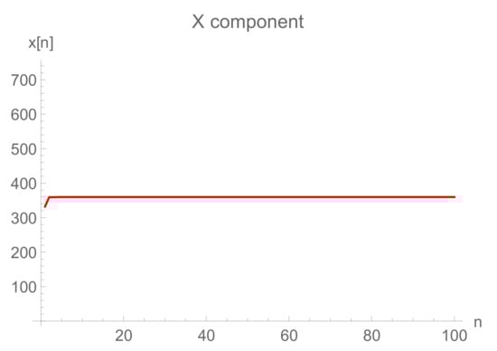
Figure 1. Graph of $x_n$ for $\alpha =167,$ $\beta =0.01,$ $\gamma =0.03,$ $\delta =0.4,$ $\zeta =155,$ $\eta =0.05,$ $\mu =0.05,$ $\epsilon =0.3,$ $\upsilon =144,$ $\rho =0.03,$ $\sigma =0.08$, $\omega =0.2$. with initial conditions $x_0=10.0,$ $y_0=20.0$ and $z_0=25.0$.

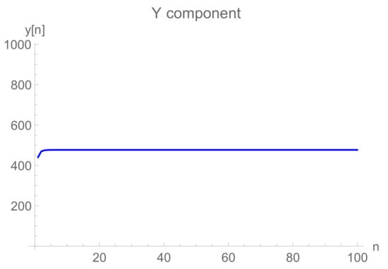
Figure 2. Graph of $y_n$ for $\alpha =167,$ $\beta =0.01,$ $\gamma =0.03,$ $\delta =0.4,$ $\zeta =155,$ $\eta =0.05,$ $\mu =0.05,$ $\epsilon =0.3,$ $\upsilon =144,$ $\rho =0.03,$ $\sigma =0.08$, $\omega =0.2$. with initial conditions $x_0=10.0,$ $y_0=20.0$ and $z_0=25.0$.

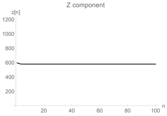
Figure 3. Graph of $z_n$ for $\alpha =167,$ $\beta =0.01,$ $\gamma =0.03,$ $\delta =0.4,$ $\zeta =155,$ $\eta =0.05,$ $\mu =0.05,$ $\epsilon =0.3,$ $\upsilon =144,$ $\rho =0.03,$ $\sigma =0.08$, $\omega =0.2$. with initial conditions $x_0=10.0,$ $y_0=20.0$ and $z_0=25.0$.

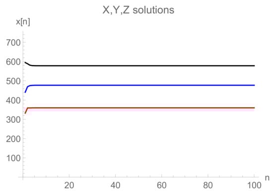
Figure 4. Combined Graph red line shows behavior of $x_n$, blue line shows behavior of $y_n$ and black line shows behavior of $z_n$ for $\alpha =167,$ $\beta =0.01,$ $\gamma =0.03,$ $\delta =0.4,$ $\zeta =155,$ $\eta =0.05,$ $\mu =0.05,$ $\epsilon =0.3,$ $\upsilon =144,$ $\rho =0.03,$ $\sigma =0.08$, $\omega =0.2$. with initial conditions $x_0=10.0,$ $y_0=20.0$ and $z_0=25.0$.

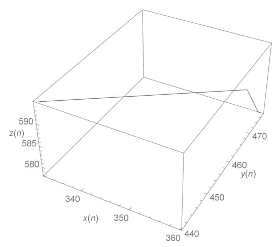
Figure 5. Attractor of $x_n,y_n$ and $z_n$ for $\alpha =167,$ $\beta =0.01,$ $\gamma =0.03,$ $\delta =0.4,$ $\zeta =155,$ $\eta =0.05,$ $\mu =0.05,$ $\epsilon =0.3,$ $\upsilon =144,$ $\rho =0.03,$ $\sigma =0.08$, $\omega =0.2$. with initial conditions $x_0=10.0,$ $y_0=20.0$ and $z_0=25.0$.

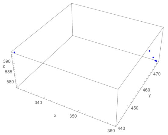
Figure 6. Attractor of $x_n,y_n$ and $z_n$ as dot graph for $\alpha =167,$ $\beta =0.01,$ $\gamma =0.03,$ $\delta =0.4,$ $\zeta =155,$ $\eta =0.05,$ $\mu =0.05,$ $\epsilon =0.3,$ $\upsilon =144,$ $\rho =0.03,$ $\sigma =0.08$, $\omega =0.2$. with initial conditions $x_0=10.0,$ $y_0=20.0$ and $z_0=25.0$.

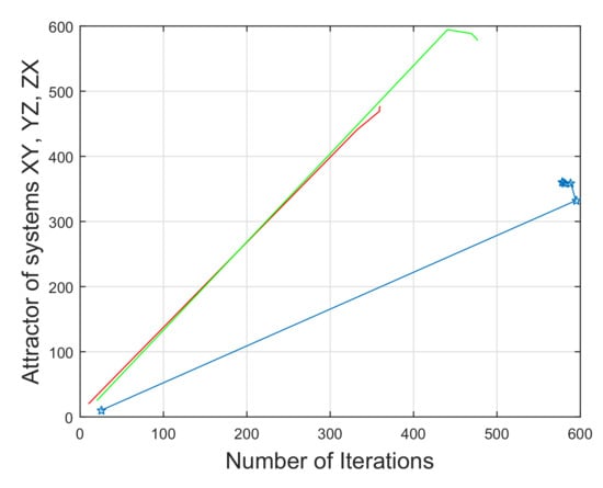
Figure 7. Combined attractor of $x_n{y}_n$(shown in blue line) $y_n{z}_n$(shown in red line) and $z_n{x}_n$ (shown in green line) for $\alpha =167,$ $\beta =0.01,$ $\gamma =0.03,$ $\delta =0.4,$ $\zeta =155,$ $\eta =0.05,$ $\mu =0.05,$ $\epsilon =0.3,$ $\upsilon =144,$ $\rho =0.03,$ $\sigma =0.08$, $\omega =0.2$. with initial conditions $x_0=10.0,$ $y_0=20.0$ and $z_0=25.0$.

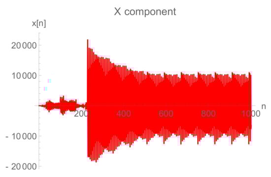
Figure 8. Graph of $x_n$ for $\alpha =2.5,$ $\beta =0.05,$ $\gamma =0.7,$ $\delta =0.6,$ $\zeta =3.5,$ $\eta =0.05,$ $\mu =0.01,$ $\epsilon =4.1,$ $\upsilon =0.09,$ $\rho =0.02,$ $\sigma =0.04$, $\omega =0.06$. with initial conditions $x_0=0.1,$ $y_0=0.02$ and $z_0=0.04$.

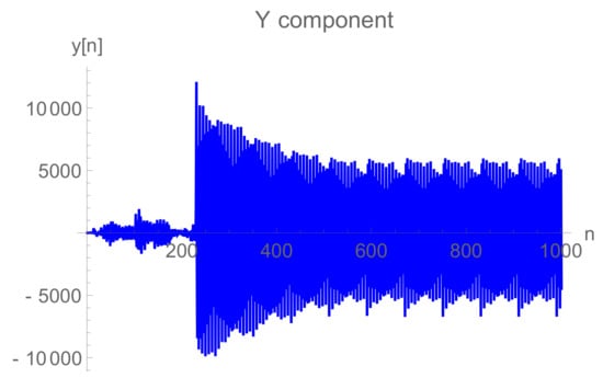
Figure 9. Graph of $y_n$ for $\alpha =2.5,$ $\beta =0.05,$ $\gamma =0.7,$ $\delta =0.6,$ $\zeta =3.5,$ $\eta =0.05,$ $\mu =0.01,$ $\epsilon =4.1,$ $\upsilon =0.09,$ $\rho =0.02,$ $\sigma =0.04$, $\omega =0.06$. with initial conditions $x_0=0.1,$ $y_0=0.02$ and $z_0=0.04$.

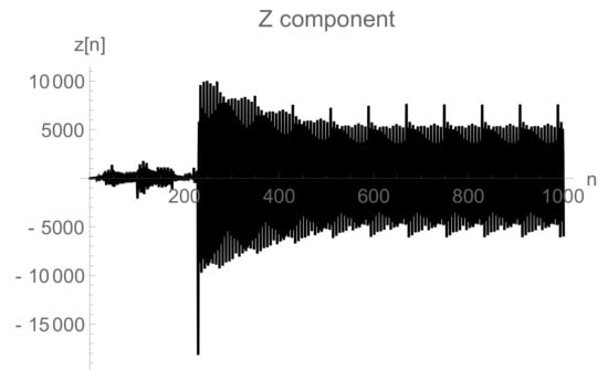
Figure 10. Graph of $z_n$ for $\alpha =2.5,$ $\beta =0.05,$ $\gamma =0.7,$ $\delta =0.6,$ $\zeta =3.5,$ $\eta =0.05,$ $\mu =0.01,$ $\epsilon =4.1,$ $\upsilon =0.09,$ $\rho =0.02,$ $\sigma =0.04$, $\omega =0.06$. with initial conditions $x_0=0.1,$ $y_0=0.02$ and $z_0=0.04$.

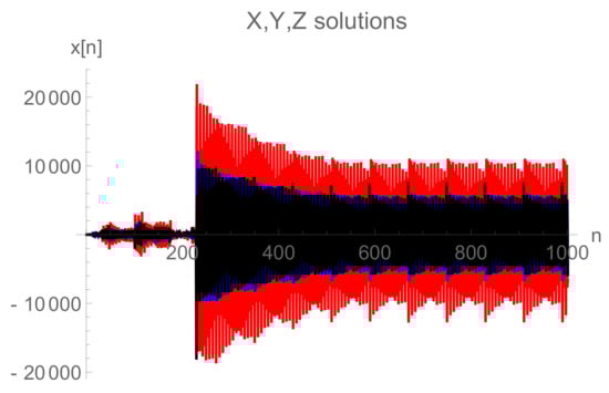
Figure 11. Combined graph of $x_n$,(shown in red line) $y_n$(shown in blue line) and $z_n$(shown in black line) for $\alpha =2.5,$ $\beta =0.05,$ $\gamma =0.7,$ $\delta =0.6,$ $\zeta =3.5,$ $\eta =0.05,$ $\mu =0.01,$ $\epsilon =4.1,$ $\upsilon =0.09,$ $\rho =0.02,$ $\sigma =0.04$, $\omega =0.06$. with initial conditions $x_0=0.1,$ $y_0=0.02$ and $z_0=0.04$.

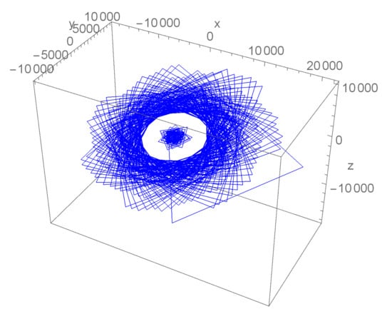
Figure 12. Graph of attractors $x_n{y}_n{z}_n$ in 3D for $\alpha =2.5,$ $\beta =0.05,$ $\gamma =0.7,$ $\delta =0.6,$ $\zeta =3.5,$ $\eta =0.05,$ $\mu =0.01,$ $\epsilon =4.1,$ $\upsilon =0.09,$ $\rho =0.02,$ $\sigma =0.04$, $\omega =0.06$. with initial conditions $x_0=0.1,$ $y_0=0.02$ and $z_0=0.04$.

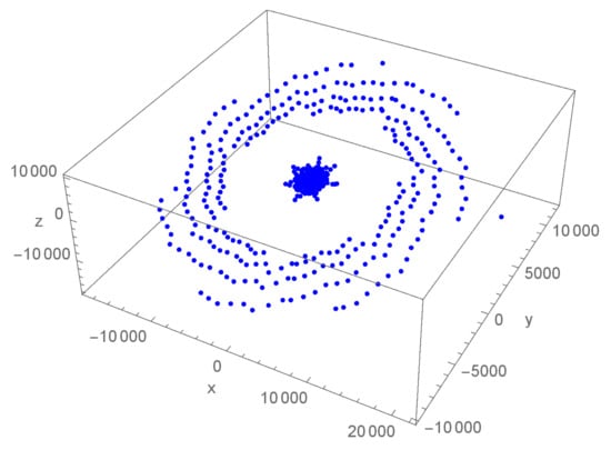
Figure 13. Graph of attractors $x_n{y}_n{z}_n$ in 3D for $\alpha =2.5,$ $\beta =0.05,$ $\gamma =0.7,$ $\delta =0.6,$ $\zeta =3.5,$ $\eta =0.05,$ $\mu =0.01,$ $\epsilon =4.1,$ $\upsilon =0.09,$ $\rho =0.02,$ $\sigma =0.04$, $\omega =0.06$. with initial conditions $x_0=0.1,$ $y_0=0.02$ and $z_0=0.04$.

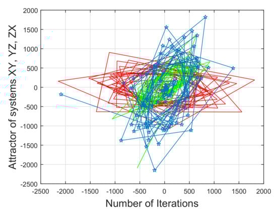
Figure 14. Graph of attractors $x_n{y}_n$(shown in blue line) $y_n{z}_n$, (shown in green line) $z_n{y}_n$(shown in red line) in 2D for $\alpha =2.5,$ $\beta =0.05,$ $\gamma =0.7,$ $\delta =0.6,$ $\zeta =3.5,$ $\eta =0.05,$ $\mu =0.01,$ $\epsilon =4.1,$ $\upsilon =0.09,$ $\rho =0.02,$ $\sigma =0.04$, $\omega =0.06$. with initial conditions $x_0=0.1,$ $y_0=0.02$ and $z_0=0.04$.

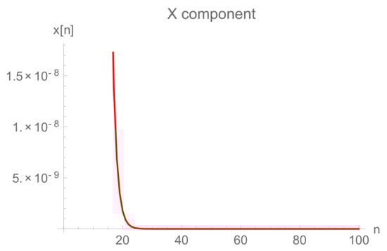
Figure 15. Graph of $x_n$ for $\alpha =0.5,$ $\beta =1.7,$ $\gamma =1.6,$ $\delta =0.3,$ $\zeta =0.7,$ $\eta =1.6,$ $\mu =2.7,$ $\epsilon =0.6,$ $\upsilon =0.8,$ $\rho =1.11,$ $\sigma =1.11$, $\omega =0.2$. with initial conditions $x_0=0.002,$ $y_0=0.0084$ and $z_0=0.0003$.

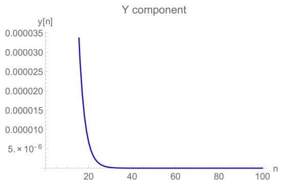
Figure 16. Graph of $y_n$ for $\alpha =0.5,$ $\beta =1.7,$ $\gamma =1.6,$ $\delta =0.3,$ $\zeta =0.7,$ $\eta =1.6,$ $\mu =2.7,$ $\epsilon =0.6,$ $\upsilon =0.8,$ $\rho =1.11,$ $\sigma =1.11$, $\omega =0.2$. with initial conditions $x_0=0.002,$ $y_0=0.0084$ and $z_0=0.0003$.

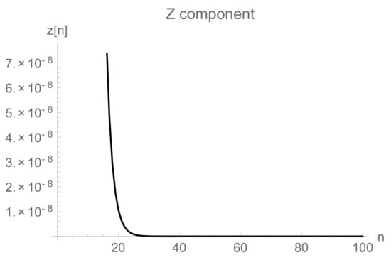
Figure 17. Graph of $z_n$ for $\alpha =0.5,$ $\beta =1.7,$ $\gamma =1.6,$ $\delta =0.3,$ $\zeta =0.7,$ $\eta =1.6,$ $\mu =2.7,$ $\epsilon =0.6,$ $\upsilon =0.8,$ $\rho =1.11,$ $\sigma =1.11$, $\omega =0.2$. with initial conditions $x_0=0.002,$ $y_0=0.0084$ and $z_0=0.0003$.

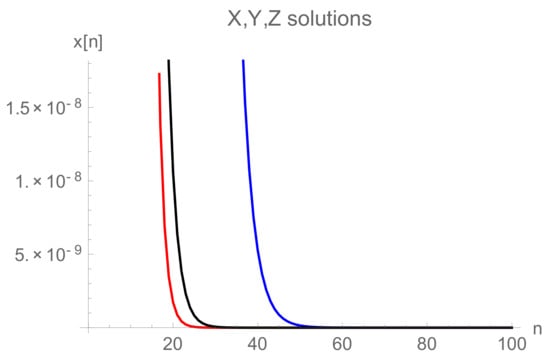
Figure 18. Combined graph of solution behavior of $x_n$ is shown in red line, and for $y_n$ is shown in blue line, for $z_n$ is shown in black line when $\alpha =0.5,$ $\beta =1.7,$ $\gamma =1.6,$ $\delta =0.3,$ $\zeta =0.7,$ $\eta =1.6,$ $\mu =2.7,$ $\epsilon =0.6,$ $\upsilon =0.8,$ $\rho =1.11,$ $\sigma =1.11$, $\omega =0.2$. with initial conditions $x_0=0.002,$ $y_0=0.0084$ and $z_0=0.0003$.

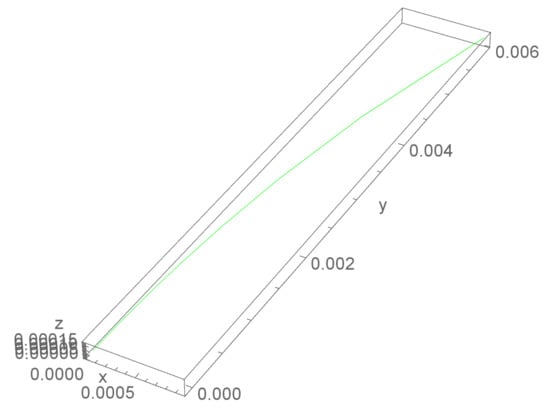
Figure 19. Attractor of system $(3)$ when $\alpha =0.5,$ $\beta =1.7,$ $\gamma =1.6,$ $\delta =0.3,$ $\zeta =0.7,$ $\eta =1.6,$ $\mu =2.7,$ $\epsilon =0.6,$ $\upsilon =0.8,$ $\rho =1.11,$ $\sigma =1.11$, $\omega =0.2$. with initial conditions $x_0=0.002,$ $y_0=0.0084$ and $z_0=0.0003$.

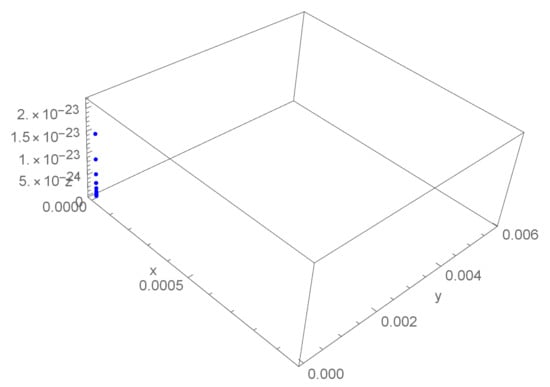
Figure 20. Attractor of system $(3)$ in 3D when $\alpha =0.5,$ $\beta =1.7,$ $\gamma =1.6,$ $\delta =0.3,$ $\zeta =0.7,$ $\eta =1.6,$ $\mu =2.7,$ $\epsilon =0.6,$ $\upsilon =0.8,$ $\rho =1.11,$ $\sigma =1.11$, $\omega =0.2$. with initial conditions $x_0=0.002,$ $y_0=0.0084$ and $z_0=0.0003$.

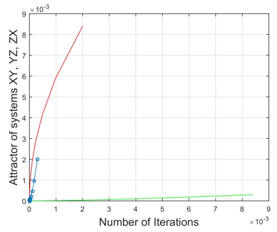
Figure 21. Attractors of system $(3)$ $x_n{y}_n$(shown in blue line) $y_n{z}_n$(shown in green line) $z_n{y}_n$(shown in red line) in 2D when $\alpha =0.5,$ $\beta =1.7,$ $\gamma =1.6,$ $\delta =0.3,$ $\zeta =0.7,$ $\eta =1.6,$ $\mu =2.7,$ $\epsilon =0.6,$ $\upsilon =0.8,$ $\rho =1.11,$ $\sigma =1.11$, $\omega =0.2$. with initial conditions $x_0=0.002,$ $y_0=0.0084$ and $z_0=0.0003$.

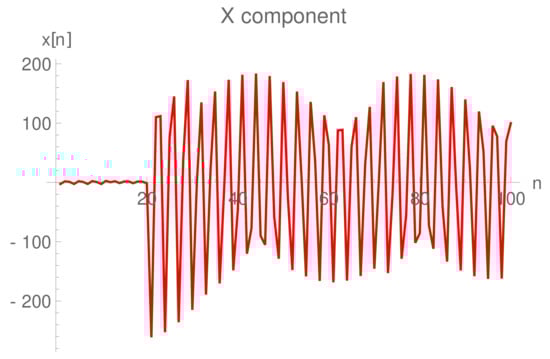
Figure 22. Graph of $x_n$ for $\alpha =0.00001,$ $\beta =2.0,$ $\gamma =3.0,$ $\delta =4.0,$ $\zeta =0.00005,$ $\eta =6.0,$ $\mu =7.0,$ $\epsilon =0.00009,$ $\upsilon =8.0,$ $\rho =10.0,$ $\sigma =11.0$, $\omega =12.0$. with initial conditions $x_0=1.0,$ $y_0=2.0$ and $z_0=3.0$.

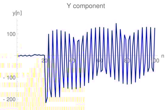
Figure 23. Graph of $y_n$ for $\alpha =0.00001,$ $\beta =2.0,$ $\gamma =3.0,$ $\delta =4.0,$ $\zeta =0.00005,$ $\eta =6.0,$ $\mu =7.0,$ $\epsilon =0.00009,$ $\upsilon =8.0,$ $\rho =10.0,$ $\sigma =11.0$, $\omega =12.0$. with initial conditions $x_0=1.0,$ $y_0=2.0$ and $z_0=3.0$.

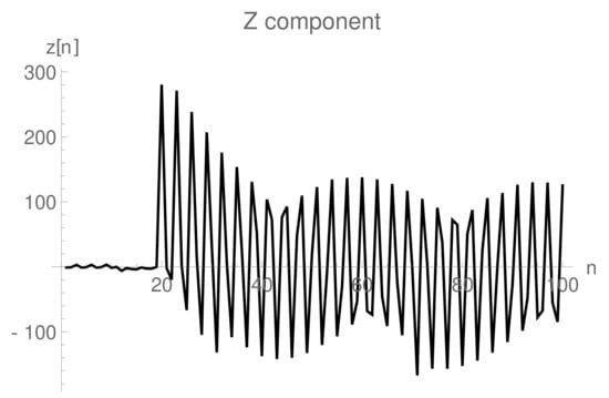
Figure 24. Graph of $z_n$ for $\alpha =0.00001,$ $\beta =2.0,$ $\gamma =3.0,$ $\delta =4.0,$ $\zeta =0.00005,$ $\eta =6.0,$ $\mu =7.0,$ $\epsilon =0.00009,$ $\upsilon =8.0,$ $\rho =10.0,$ $\sigma =11.0$, $\omega =12.0$. with initial conditions $x_0=1.0,$ $y_0=2.0$ and $z_0=3.0$.

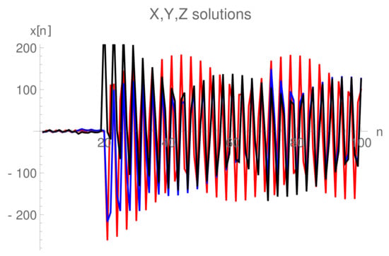
Figure 25. Combined Graph of behavior of solution of $x_n$(shown in red line) $y_n$(shown in blue line) and $z_n$(shown in black line) for $\alpha =0.00001,$ $\beta =2.0,$ $\gamma =3.0,$ $\delta =4.0,$ $\zeta =0.00005,$ $\eta =6.0,$ $\mu =7.0,$ $\epsilon =0.00009,$ $\upsilon =8.0,$ $\rho =10.0,$ $\sigma =11.0$, $\omega =12.0$. with initial conditions $x_0=1.0,$ $y_0=2.0$ and $z_0=3.0$.

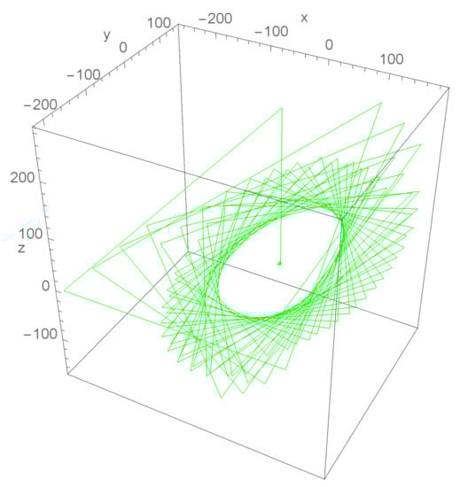
Figure 26. 3D attractor of $x_n,y_n,z_n$ for $\alpha =0.00001,$ $\beta =2.0,$ $\gamma =3.0,$ $\delta =4.0,$ $\zeta =0.00005,$ $\eta =6.0,$ $\mu =7.0,$ $\epsilon =0.00009,$ $\upsilon =8.0,$ $\rho =10.0,$ $\sigma =11.0$, $\omega =12.0$. with initial conditions $x_0=1.0,$ $y_0=2.0$ and $z_0=3.0$.

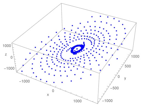
Figure 27. 3D attractor dot plot of $x_n,y_n,z_n$ for $\alpha =0.00001,$ $\beta =2.0,$ $\gamma =3.0,$ $\delta =4.0,$ $\zeta =0.00005,$ $\eta =6.0,$ $\mu =7.0,$ $\epsilon =0.00009,$ $\upsilon =8.0,$ $\rho =10.0,$ $\sigma =11.0$, $\omega =12.0$. with initial conditions $x_0=1.0,$ $y_0=2.0$ and $z_0=3.0$.

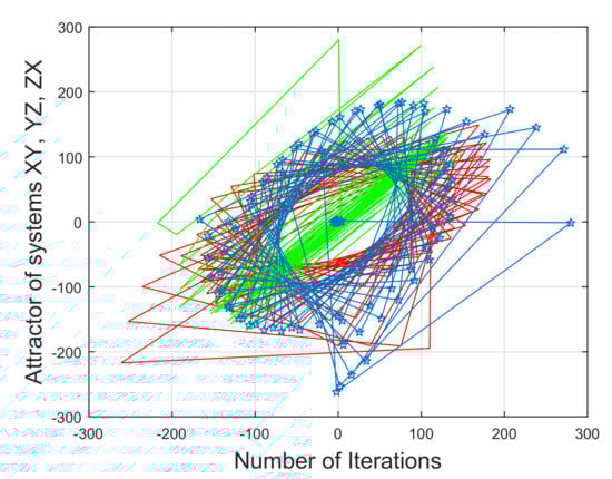
Figure 28. Combined attractors $x_n{y}_n$(shown in blue line) $y_n{z}_n$(shown in green line) $z_n{y}_n$ (shown in red line) of system $(3)$ in 2D for $\alpha =0.00001,$ $\beta =2.0,$ $\gamma =3.0,$ $\delta =4.0,$ $\zeta =0.00005,$ $\eta =6.0,$ $\mu =7.0,$ $\epsilon =0.00009,$ $\upsilon =8.0,$ $\rho =10.0,$ $\sigma =11.0$, $\omega =12.0$. with initial conditions $x_0=1.0,$ $y_0=2.0$ and $z_0=3.0$.

7. Conclusions

This research work is associated to the qualitative conduct of a possible discrete-time Lotka–Volterra model. The continuous form of this model is given by:

$$\begin{array}{ccc}\hfill \frac{dx}{dt}& =& rx(1-\frac{x}{k})-\frac{\xi xy}{1+u_1\xi x}-\frac{\eta xz}{1+u_2\eta x}\hfill \\ \hfill \frac{dy}{dt}& =& {-py+N}_{1}y(1-\frac{y}{k_y}{)-c}_{1}yz\hfill \\ \hfill \frac{dz}{dt}& =& {-qz+N}_{2}z(1-\frac{z}{k_z}{)-c}_{2}yz\hfill \end{array}$$

The rate of intrinsic growth of prey is r where $\zeta$ and $\eta$ measure the efficiency of the looking and the catch of predators $yandz$ separately. $u_1$ and $u_2$ represent the handling and digestion rates of predators. Without prey x constants, p and q are the death rates of predators $y,z$ individually. The discrete-time LV model $(3)$ is obtained by Euler’s method and the nonstandard finite difference scheme, such that the fixed points in both cases have been preserved. With the help of linear stability analysis, a three-dimensional discrete-time system can be analyzed in terms of its dynamics of positive equilibrium. We have proven that the system $(3)$ has eight equilibrium points, from which one of them is unique and other in certain parametric conditions is stable locally and asymptotically. A major contribution to this research is proving that the unique positive equilibrium point

$$V=\left(\begin{array}{c}\frac{-\zeta \beta \omega +\zeta \gamma \sigma +\alpha \epsilon \omega -\alpha \mu \sigma +\beta \mu \upsilon -\epsilon \gamma \upsilon -\beta \mu +\beta \omega +\epsilon \gamma -\epsilon \omega -\gamma \sigma +\mu \sigma }{\beta \eta \omega -\beta \mu \rho +\delta \epsilon \omega -\delta \mu \sigma +\epsilon \gamma \rho -\eta \gamma \sigma },\\ \frac{-\zeta \delta \omega +\zeta \gamma \rho +\alpha \eta \omega -\alpha \mu \rho -\delta \mu \upsilon -\eta \gamma \upsilon +\delta \mu -\delta \omega +\eta \gamma -\eta \omega -\gamma \rho +\mu \rho }{\beta \eta \omega -\beta \mu \rho +\delta \epsilon \omega -\delta \mu \sigma +\epsilon \gamma \rho -\eta \gamma \sigma },\\ \frac{-\zeta \beta \rho +\zeta \delta \sigma +\alpha \epsilon \rho -\alpha \eta \sigma -\beta \eta \upsilon -\delta \epsilon \upsilon -\beta \eta -\beta \rho +\delta \epsilon -\delta \sigma +\epsilon \sigma -\eta \sigma }{\beta \eta \omega -\beta \mu \rho +\delta \epsilon \omega -\delta \mu \sigma +\epsilon \gamma \rho -\eta \gamma \sigma }\end{array}\right)$$

of the system $(3)$ exists and is globally asymptotically stable. In addition, the rate at which the solution converges to the unique positive equilibrium point of the system $(3)$ was also studied. Dynamical systems theory aims to predict the global behavior of a system based on its current state. It is possible to determine the long-term behaviors of the system by determining which parametric conditions lead to these long-term behaviors. Nonlinear dynamical systems must be discussed in terms of their global behavior. Additionally, we found the rate of convergence of a solution that converges to the unique positive equilibrium point of system $(3)$. Finally, a couple of illustrative numerical examples are outfitted to help our theoretical conversation in the Numerical Debate section. The obtained results can further be useful to find the bifurcation parameter and maximum Lyapunov exponent (MLE).

8. Future Work

In our future work, we will study some more qualitative properties such as bifurcation analysis, chaos control, and the maximum Lyapunov exponent of the obtained discrete model. It will be interesting to find the bifurcation parameter among so many other parameters. Some interesting numerical simulations with the help of MATHEMATICA presenting bifurcation and chaos control will also be part of our future goals.

References

- Freedman, H.I. Deterministic Mathematical Models in Population Ecology; Marcel Dekker, Inc.: New York, NY, USA, 1980. [Google Scholar]
- Allen, L.J.S. An Introduction to Mathematical Biology; Pearson Prentice Hall: Hoboken, NJ, USA, 2007. [Google Scholar]
- Krebs, W. A General Predator-Prey Model. Math. Comp. Model. Dyn. Syst. 2003, 9, 387–401. [Google Scholar] [CrossRef]
- Edelstein-Keshet, L. Mathematical Models in Biology; McGraw-Hill: New York, NY, USA, 1988. [Google Scholar]
- Akgül, A.; Sarbaz, H.; Khoshnaw, A. Application of fractional derivative on non-linear biochemical reaction models. Int. J. Intell. Netw. 2020, 1, 52–58. [Google Scholar] [CrossRef]
- Sintunavarat, W.; Turab, A. A unified fixed point approach to study the existence of solutions for a class of fractional boundary value problems arising in a chemical graph theory. PLoS ONE 2022, 17, e0270148. [Google Scholar] [CrossRef]
- Kang, H.; Pesin, Y. Dynamics of a discrete Brusselator model: Escape to infinity and Julia set. Milan J. Math. 2005, 73, 1–17. [Google Scholar] [CrossRef]
- Wikan, A.; Mjølhus, E. Over-compensatory recruitment and generation delay in discrete age-structured population models. J. Math. Biol. 1996, 35, 195–239. [Google Scholar]
- Din, Q.; Elsayed, E.M. Stability analysis of a discrete ecological model. Comput. Ecol. Softw. 2014, 4, 89–103. [Google Scholar]
- Levin, S.A.; Goodyear, C.P. Analysis of an age-structured fishery model. J. Math. Biol. 1980, 9, 245–274. [Google Scholar] [CrossRef]
- Kulenovic, M.R.S.; Ladas, G. Dynamics of Second Order Rational Difference Equations; Chapman and Hall/CRC: Boca Raton, FL, USA, 2002. [Google Scholar]
- Elsayed, E.M.; Khaliq, A. The Dynamics and Global Attractivity of a Rational Difference Equation. Adv. Stud. Contemp. Math. 2016, 26, 183–202. [Google Scholar]
- Gakkhar, S.; Singh, B.; Naji, R.K. Dynamical behavior of two predators competing over a single prey. BioSystems 2007, 90, 808–817. [Google Scholar] [CrossRef]
- Khan, A.Q.; Qureshi, M.N. Global Dynamics and Bifurcation Analysis of a Two-Dimensional Discrete-Time Lotka-Volterra Model. Complexity 2018, 2018, 7101505. [Google Scholar] [CrossRef]
- Tang, X.; Zou, X. On positive periodic solutions of Lotka-Volterra competition systems with deviating arguments. Pro. Am. Math. Soc. 2006, 134, 29672–29974. [Google Scholar] [CrossRef]
- Alebraheem, J.; Abu-Hasan, Y. Persistence of Predators in a Two Predators- One Prey Model with Non-Periodic Solution. Appl. Math. Sci. 2012, 6, 943–956. [Google Scholar]
- Huo, H.F.; Ma, Z.P.; Liu, C.Y. Persistence and Stability for a Generalized Leslie-Gower Model with Stage Structure and Dispersal. Abstr. Appl. Anal. 2009, 135843. [Google Scholar] [CrossRef]
- Belhannache, F.; Touafek, N.; Abo-Zeid, R. Dynamics of a third-order rational difference equation. Bull. Math. Soc. Sci. Math. Roum. Tome 2016, 59, 13–22. [Google Scholar]
- Dubey, B.; Upadhyay, R.K. Persistence and Extinction of One-Prey and Two-Predators System. Nonlinear Anal. Model. Control 2004, 9, 307–329. [Google Scholar] [CrossRef]
- Ahmad, S. On the nonautonomous Lotka-Volterra competition equation. Proc. Am. Math. Soc. 1993, 117, 199–204. [Google Scholar] [CrossRef]
- Kocic, V.L.; Ladas, G. Global Behavior of Nonlinear Difference Equations of Higher Order with Applications; Kluwer Academic Publishers: Dordrecht, The Netherlands, 1993. [Google Scholar]
- Zhang, Q.; Yang, L.; Liu, J. Dynamics of a system of rational third order difference equation. Adv. Differ. Equ. 2012, 2012, 136. [Google Scholar] [CrossRef]
- Grove, E.A.; Ladas, G. Periodicities in Nonlinear Difference Equations; Chapman and Hall/CRC: Boca Raton, FL, USA, 2005. [Google Scholar]
- Sedaghat, H. Nonlinear Difference Equations: Theory with Applications to Social Science Models; Kluwer Academic Publishers: Dordreacht, The Netherlands, 2003. [Google Scholar]
- Thai, T.H.; Khuong, V.V. Stability analysis of a system of second-order difference equations. Math. Methods Appl. Sci. 2016, 39, 3691–3700. [Google Scholar] [CrossRef]
- Elaydi, S. An Introduction to Difference Equations, 2nd ed.; Springer Science+Business Media, Inc.: New York, NY, USA, 2005. [Google Scholar]
- Tanaka, Y. Brouwer’s fixed point theorem with isolated fixed points and his Fan theorem. Int. Sch. Res. Netw. 2012, 2012, 843256. [Google Scholar] [CrossRef]
- Elsayed, E.M. Solutions of Rational Difference System of Order Two. Math. Comput. Model. 2012, 55, 378–384. [Google Scholar] [CrossRef]
- Elsayed, E.M. Behavior and expression of the solutions of some rational difference equations. J. Comput. Anal. Appl. 2013, 15, 73–81. [Google Scholar]
- Khaliq, A.; Alayachi, H.S.; Zubair, M.; Rohail, M.; Khan, A.Q. On stability analysis of a class of three dimensional system of exponential difference equations. 2022. to be appeared. [Google Scholar]
- Elsayed, E.M. Dynamics and Behavior of a Higher Order Rational Difference Equation. J. Nonlinear Sci. Appl. 2016, 9, 1463–1474. [Google Scholar] [CrossRef]
- Elsayed, E.M.; Ahmed, A.M. Dynamics of a three-dimensional systems of rational difference equations. Math. Methods Appl. Sci. 2016, 39, 1026–1038. [Google Scholar] [CrossRef]
- Elsayed, E.M.; Alghamdi, A. Dynamics and Global Stability of Higher Order Nonlinear Difference Equation. J. Comput. Appl. 2016, 21, 493–503. [Google Scholar]
- Din, Q. Dynamics of a discrete Lotka-Volterra model. Adv. Differ. Equ. 2013, 2013, 95. [Google Scholar] [CrossRef]
- Pituk, M. More on Poincare’s and Perron’s Theorems for Difference Equations. J. Differ. Equ. Appl. 2002, 8, 201–216. [Google Scholar] [CrossRef]
Publisher’s Note: MDPI stays neutral with regard to jurisdictional claims in published maps and institutional affiliations. |
© 2022 by the authors. Licensee MDPI, Basel, Switzerland. This article is an open access article distributed under the terms and conditions of the Creative Commons Attribution (CC BY) license (https://creativecommons.org/licenses/by/4.0/).