Variational Estimation Methods for Sturm–Liouville Problems

Abstract

In this paper, we are concerned with approach solutions for Sturm–Liouville problems (SLP) using variational problem (VP) formulation of regular SLP. The minimization problem (MP) is also set forth, and the connection between the solution of each formulation is then proved. Variational estimations (the variational equation associated through the Euler–Lagrange variational principle and Nehari’s method, shooting method and bisection method) and iterative variational methods (He’s method and HPM) for regular RSL are unitary presented in final part of the paper, which ends with applications.

1. Introduction

Nonlinearities are different from linear type by a function, an operator or a system that is nonlinear or is the case in which only some characteristics of it are known. The existence of the solution and the dependence of conditions for solving some classes of differential equations described by an operator is specified by the general framework of the Sturm–Liouville problem, with parametric conditions at the limit. The general framework of the Sturm–Liouville problem with parametric conditions at the limit is specified in the first part of the paper. The existence of the solution and the dependence of conditions is specified through the connection between the differential operator and Green’s function. Based on the properties of Green’s function, the operator used to analyze the behavior of the solution of the parameters given by the boundary conditions is specified. Variational problems derived from the initial RSLP are outlined with different type conditions in order to estimate the solution.

Let be the operator ${\displaystyle L=-\frac{d}{dx}\left[p\left(x\right)\frac{d}{dx}\right]+\rho \left(x\right)}$ as part of the regular Sturm–Liouville problem (RSL). The Sturm–Liouville (SL) problem expressed by the differential equation and the boundary conditions

$${\displaystyle a\left(x\right)\frac{d^{2}u}{d{x}^2}+b\left(x\right)\frac{du}{dx}+c\left(x\right)u-\lambda d\left(x\right)u=0,}$$

(1)

$$\begin{array}{c}{\mathit{B}}_1:a_{1}u\left(a\right)+a_2{u}^{\prime }\left(a\right)=0,|a_1|+|a_2|\ne 0,a_1,a_2\in \mathbb{R},\hfill \\ {\mathit{B}}_2:b_{1}u\left(b\right)+b_2{u}^{\prime }\left(b\right)=0,|b_1|+|b_2|\ne 0,b_1,b_2\in \mathbb{R}\hfill \end{array}$$

(2)

could be written as

$$Lu+\lambda s\left(x\right)u=0,x\in (a,b)=I,\lambda \in \mathbb{R}$$

(3)

with $p\left(x\right)=a\left(x\right),\rho \left(x\right)=-c\left(x\right),s\left(x\right)=d\left(x\right)$ in case $b\left(x\right)=a^{\prime }\left(x\right)$ and with integrant factor $\mu =k{e}^{{\displaystyle {\int }_a^x\frac{b\left(t\right)}{a\left(t\right)}dt}}$, $p\left(x\right)=\mu a\left(x\right),\rho \left(x\right)=-\mu c\left(x\right),s\left(x\right)=\mu d\left(x\right)$ in case $b\left(x\right)\ne a^{\prime }\left(x\right)$ (see [1,2]).

The Sturm–Liouville equation is regular in the interval $[a,b]$ if the functions verify the condition $p\left(x\right)>0$ and $s\left(x\right)>0,\forall x\in I$ or $s\equiv 0$ and the operator $L:\mathcal{H}={\mathcal{L}}^2\left(I\right)\cap {\mathcal{C}}^2\left(I\right)\to {\mathcal{L}}^2\left(I\right)$ is self-adjoint with real eigenvalues and orthogonal eigenfunctions in space ${\mathcal{L}}_s^2\left(I\right)$ according to the inner product

$$⟨f,g⟩={\int }_a^{b}fg\mathrm{d}xf,g\in {\mathcal{L}}^2\left(I\right);{⟨f,g⟩}_s={\int }_a^{b}sfg\mathrm{d}x\mathrm{in}{\mathcal{L}}_s^2\left(I\right).$$

(4)

and for a given $\lambda$, there exist two linearly independent solutions of a $RSL$ equation in the I interval, ${\mathcal{L}}^2\left(I\right)=\left\{f:I\to \mathbb{R},{\int }_a^b{\left|f\left(x\right)\right|}^2\mathrm{d}x<\infty \right\}$.

We denote $D\left(L\right)$ as the domain of L that is defined by

$$\begin{array}{c}D\left(L\right)=\left\{\mathrm{y}\in \mathcal{C}\left([a,b]\right),y^{″}\in {\mathcal{L}}^2\left(I\right),\mathrm{y}\mathrm{satisfies}{B}_1,B_2\right\}\mathrm{for}\mathrm{general}\mathrm{case}\hfill \\ D\left(L\right)=\left\{\mathrm{y}\in \mathcal{C}\left([a,b]\right),{\left(p{y}^{\prime }\right)}^{\prime }\in \mathcal{C}\left([a,b]\right),\mathrm{y}\mathrm{satisfies}{B}_1,B_2\right\}\mathrm{for}\mathrm{regular}\mathrm{case}.\end{array}$$

(5)

The adjoint operator, $L^{\ast }$, associated to the operator L verifies $⟨Lf,g⟩=⟨f,L^{\ast }g⟩,\forall f,g\in \mathcal{H}$ and L is self-adjoint if $L=L^{\ast }$. Additionally, the operator L is symmetric if $⟨Lf,g⟩=⟨f,Lg⟩,\forall f,g\in D\left(L\right)$. For the operator defined for SL problems, one obtains

$${\displaystyle ⟨g,Lf⟩-⟨f,Lg⟩=\left[p\left(f^{\prime }g-f{g}^{\prime }\right)\right]{|}_a^b,\forall f,g\in D\left(L\right)}$$

and the condition $⟨Lf,g⟩=⟨f,Lg⟩$ holds if ${\left.p\left(f{g}^{\prime }-f^{\prime }g\right)\right|}_a^b=0$ verified in $D\left(L\right)$ and the Lagrange identity is expressed by

$$gLf-fLg={\left[p\left(f{g}^{\prime }-f^{\prime }g\right)\right]}^{\prime },\forall f,g\in D\left(L\right).$$

Remark 1. 

L for SL problems is the self-adjoint operator if

$${\left.p\left(u^{\prime }v-u{v}^{\prime }\right)\right|}_a^b=p\left(b\right)u^{\prime }\left(b\right)v\left(b\right)-p\left(a\right)u^{\prime }\left(a\right)v\left(a\right)=0.$$

(6)

For example, for$p\left(b\right)=p\left(a\right)$and periodic conditions

$$\begin{array}{cc}\hfill u\left(a\right)=u\left(b\right)=A,& u^{\prime }\left(a\right)=u^{\prime }\left(b\right)=B\hfill \end{array}$$

or antiperiodic conditions

$$\begin{array}{cc}\hfill u\left(a\right)=-u\left(b\right)=A,& u^{\prime }\left(a\right)=-u^{\prime }\left(b\right)=B\hfill \end{array}$$

the operator L is self-adjoint.

The RSL eigenvalue problem is to find $v\in D\left(L\right)$ such that for $Lv+\lambda v=0$ with $\lambda$, the eigenvalue associated with v is the eigenfunction. For RSL problems, all the eigenvalues are real and positive [3,4,5], and there exists an infinite number of eigenvalues. The sequence of the eigenvalues ${\left({\lambda }_n\right)}_n$ is considered such that ${\lambda }_0<{\lambda }_1<\dots <{\lambda }_n<\dots$ with $\underset{x\to \infty }{lim}{\lambda }_n=\infty$. For each eigenvalue ${\lambda }_n$, the corresponding eigenfunction $v_n$ is unique up to a constant factor and has exactly $n-1$ zeros in interval $(a,b)$. The set $V=\left\{{\left(v_n\right)}_n,v_n\in D\left(L\right)\right\}$ is complete in the $D\left(L\right)$ space, and the solution of RSL is represented by a generalized Fourier series of the eigenfunction

$$u=\sum _{n=1}^{\infty }{c}_n{v}_n\left(x\right).$$

(7)

2. General Framework of SLPs

In this section, we will mention certain conditions that the functions defining the operator L fulfill for different SL or RSL problems.

A second method to find the solution of a RSL problem, different from the generalized Fourier series development, is described using the Green function and two linear independent solutions. The section ends with the analysis of the Fourier equation with different types of boundary conditions.

Remark 2. 

For Sturm–Liouville problems, we consider two types of assumptions that are usually used (see [4])

• General assumptions:

  (1) 

  $p\left(x\right)\in C\left(\right[a,b\left]\right)$, differentiable in $x=a$, $p\left(x\right)\ne 0$$\forall x\in (a,b]$ with $p\left(a\right)=0$, $p^{\prime }\left(a\right)\ne 0$.

  For $p\left(x\right)=(x-a)\phi \left(x\right)$, we suppose $\phi \in C\left(\right[a,b\left]\right)$, $\phi \left(x\right)\ne 0,\forall x\in [a,b]$

  (2) 

  $\rho ,f\in C\left(\right[a,b\left]\right)$.

• RSL assumptions

  (1) 

  $p\left(x\right)>0$ and $s\left(x\right)>0$ or $s\equiv 0$ on $[a,b]$;

  (2) 

  $p,\rho ,s\in C\left(\right[a,b\left]\right)$;

  (3) 

  $a_1,a_2,b_1,b_2\in \mathbb{R}$;

  (4) 

  $p,\rho ,s$continuously differentiable on$[a,b]$.

Known equations, such as Fourier, Graetz–Nusslet, Collatz and Airy equations, for which RSL assumptions are verified, are given in Table 1, and the first eigenvalues and eigenfunctions are depicted in Figure 1 and Figure 2.

Table 1. Examples of regular Sturm–Liouville problems.

Equation	Associated Functions	Name
${\displaystyle -u^{″}+\lambda u=f,x\in (a,b)}$	$p\equiv 1,s\equiv 1,\rho \equiv 0$	Fourier
${\displaystyle -{\left(x{u}^{\prime }\right)}^{\prime }=2\lambda x(1-x^2)u,x\in (0,1)}$	$p\left(x\right)=x,s\left(x\right)=2x(1-x^2)$	Graetz–Nusselt
${\displaystyle -x^6{u}^{″}+(3/4)x^{4}u=\lambda u,x\in (1,2)}$	${\displaystyle p\left(x\right)=x^6,s\left(x\right)=\frac{3}{4}{x}^4}$	Collatz
${\displaystyle -u^{″}+xu=\lambda xu,x\in (0,1)}$	$p\left(x\right)=x,s\left(x\right)=2x(1-x^2)$	Airy

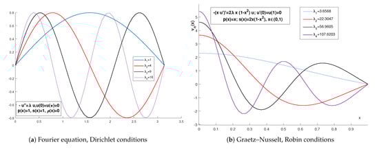
Figure 1. (a) Fourier equation; (b) Graetz–Nusselt equation.

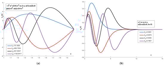
Figure 2. (a) Collatz problem; (b) Airy problem.

Some other known equations, such as the Legendre differential equation, Chebysev’s differential equation or Bessel equation, must be transformed into the Sturm–Liouville form that we considered in (3). These forms are specified in Table 2. Other SL equations for which general assumptions are fulfilled are exemplified in Table 3.

Table 2. Examples of differential equations and their SL form.

Type	Equation	Sturm–Liouville Form
Legendre	${\displaystyle -u^{″}-\frac{2x}{1-x^2}+\frac{\mu }{1-x^2}u=0,}$	$-{\left((1-x^2)u^{\prime }\right)}^{\prime }+\mu u=0$
Chebysev	${\displaystyle -(1-x^2)u^{″}-x{u}^{\prime }+n^{2}u=0}$	${\displaystyle -{\left(\sqrt{1-x^2}{u}^{\prime }\right)}^{\prime }=\frac{n^2}{\sqrt{1-x^2}}u}$
Bessel	${\displaystyle x^2{u}^{″}+x{u}^{\prime }+({\lambda }^2-n^2)y=0,}$	${\displaystyle -(x{u^{\prime })}^{\prime }+\frac{n^2}{x}u={\lambda }^{2}xu}$

Table 3. Examples of Sturm–Liouville problems.

$-{(sin\left(x\right)u^{\prime })}^{\prime }+cos\left(x\right)u=\lambda x^{2}u,x\in (0,b)$	$p=sin\left(x\right),\rho =cos\left(x\right)s=x^2$
$-{\left(x^2{u}^{\prime }\right)}^{\prime }-xsin\left(x\right)u=\lambda xu,x\in (0,b)$	$p=x,s=2x(1-x^2)$

For an example of a singular SL, a discontinuity on the middle of the interval is considered $[a,b]$, $x_0=(b-a)/2$, with $\rho \left(x\right)\equiv 0$ and $p\left(x\right)=\left\{\begin{array}{c}1,x\in \left[0,x_0\right)\hfill \\ c^2,x\in \left[x_0,1\right]\hfill \end{array}\right.$, $c\ne 0,c\ne 1$.

The problem to solve is $Lu+\lambda u=0,u\left(0\right)=u\left(1\right)=0$ and with $u\left(x_{0-}\right)-u\left(x_{0+}\right)=0$, $u^{\prime }\left(x_{0-}\right)-c^2{u}^{\prime }\left(x_{0+}\right)=0$ transmission conditions.

The asymptotic behavior of the eigenvalues leads to ${\displaystyle \frac{{\lambda }_n}{n^2}\to {\left(\frac{2\pi c}{1+c}\right)}^2,}$ as $n\to \infty$.

2.1. Resolvent Operator and Green Function

This RSL problem is solved using a Green function solution for the resolvent operator $R\left(\lambda \right)={(L+\lambda I)}^{-1}$ of the form

$$R\left(\lambda \right)f=\frac{{\phi }_{\lambda }\left(x\right)}{\omega \left(\lambda \right)}{\int }_a^{x}f\left(t\right){\psi }_{\lambda }\left(t\right)dt+\frac{{\psi }_{\lambda }\left(x\right)}{\omega \left(\lambda \right)}{\int }_x^{b}f\left(t\right){\phi }_{\lambda }\left(t\right)dt$$

(8)

where ${\psi }_{\lambda }$, ${\phi }_{\lambda }$ are non-trivial classical solutions of $(L+\lambda I)f=0$ which satisfy

$$\begin{array}{cc}\hfill & a_1{\phi }_{\lambda }\left(a\right)+a_2{\phi }_{\lambda }^{\prime }\left(a\right)=0\hfill \\ \hfill & b_1{\psi }_{\lambda }\left(b\right)+b_2{\psi }_{\lambda }^{\prime }\left(b\right)=0\hfill \end{array}$$

(9)

A simple normalization that eliminates some complexity can be specified by requiring

$$\begin{array}{cc}\hfill & {\phi }_{\lambda }\left(a\right)=a_2,{\phi }_{\lambda }^{\prime }\left(a\right)=-a_1\hfill \\ \hfill & {\psi }_{\lambda }\left(b\right)=b_2,{\psi }_{\lambda }^{\prime }\left(b\right)=-b_1\hfill \end{array}$$

(10)

Then, the Wronskian $\omega \left(\lambda \right)=v_1\left(x\right)v_2^{\prime }\left(x\right)-v_1^{\prime }\left(x\right)v_2\left(x\right)$ of these solutions is a function that depends only on $\lambda$:

$$\omega \left(\lambda \right)=\left(p{\phi }_{\lambda }^{\prime }\right){\psi }_{\lambda }-{\phi }_{\lambda }\left(p{\psi }_{\lambda }^{\prime }\right)$$

(11)

Therefore, $\omega \left(\lambda \right)\ne 0,\forall x\in [a,b]$ or $\omega \left(\lambda \right)\equiv 0$. The Wronskian vanishes if $\left\{{\phi }_{\lambda },{\psi }_{\lambda }\right\}$ is a dependent set of functions of x, which is precisely when both functions satisfy $(L+\lambda I)h=0$ as well as the specified conditions at $x=a$ and $x=b$, meaning $\lambda$ is an eigenvalue of L (see [6]).

For the RSL case, the equation $Lu=0$ has two linear independent solutions, $v_1$ and $v_2$ such that $a_1{v}_1\left(a\right)+a_2{v}_1^{\prime }\left(a\right)=0,b_1{v}_2\left(b\right)+b_2{v}_2^{\prime }\left(b\right)=0,$ the Green function $G:[a,b]\times [a,b]\to \mathbb{R}$,

$$G(x,y)=\left\{\begin{array}{c}{v}_1\left(y\right)v_2\left(x\right)/m,a\le y\le x\le b\hfill \\ -v_1\left(x\right)v_2\left(y\right)/m,a\le x\le y\le b\hfill \end{array}\right.,$$

(12)

$m=p\left(x\right)\omega \left(\lambda \right)$ has the properties

(i)

$G\in C^1\left({[a,b]}^2\right)$, $G(x,y)=G(y,x)$ and satisfies the boundary conditions according to each variable;

(ii)

$G\in C^2\left({[a,b]}^2\setminus M\right)$, with $L_{\rho }G\equiv -p\left(x\right)G_{xx}(x,y)-p^{\prime }\left(x\right)G_x(x,y)+\rho \left(x\right)G(x,y)=0$ over ${[a,b]}^2\setminus M$ and $M=\left\{\right(x,y)\mid x=y\}$;

(iii)

${\displaystyle G_x\left(y^{+},y\right)-G_x\left(y^{-},y\right)=\underset{\begin{array}{c}\epsilon \to 0\\ \epsilon >0\end{array}}{lim}\left[G_x(y+\epsilon ,y)-G_x(y-\epsilon ,y)\right]=\frac{1}{p\left(x\right)}}$, $G_x$ is discontinuous on M.

Now let T be the operator ${\displaystyle Tu\left(x\right)={\int }_a^{b}G(x,y)u\left(y\right)dy}$ defined on $C[a,b]$. Using the properties of the Green function G and the continuity of u, one obtains that Tu$\in C^2[a,b]$ and is the solution of the equation $Lu=f$. The function Tu satisfies the same boundary conditions as $u\in C^2[a,b]$, then $T\left(Lu\right)\left(x\right)=u\left(x\right)$, and T is the inverse operator of L. The problem of eigenvalues and eigenfunctions $Lu+\lambda u=0,B_{1}u\left(a\right)=0;B_{2}u\left(b\right)=0$ becomes $Tu=\mu u,$ with $\mu =-1/\lambda$. For results for the construction of the operator T for fractional SLPs, see [7,8].

Remark 3 

(Rayleigh quotient). The eigenvalues of the operator L are lower bounded by a real constant. The smallest eigenvalue of the SL eigenvalue problem satisfies

$$\begin{array}{c}\hfill {\displaystyle {\lambda }_0=\underset{\begin{array}{c}u\ne 0\\ u\in D\left(L\right)\end{array}}{min}\frac{⟨Lu,u⟩}{{⟨u,u⟩}_s}=\underset{\begin{array}{c}u\ne 0\\ u\in D\left(L\right)\end{array}}{min}\frac{-{\left.pu{u}^{\prime }\right|}_a^b+{\int }_a^{b}p{\left(u^{\prime }\right)}^2+\rho u^{2}dx}{{\int }_a^b{u}^{2}sdx}}\end{array}$$

(13)

and the minimum $u_0$ is achieved if $u_0$ is the eigenfunction corresponding to ${\lambda }_0$.

2.2. Sturm–Liouville Fourier Problems

Consider the operator $L=-\frac{d}{dx}\left[p\left(x\right)\frac{d}{dx}\right]+\rho \left(x\right)$ and nonhomogeneous equation $Lu+\lambda s\left(x\right)u=f\left(x\right)$ with functions $p\left(x\right)$ smooth, $\rho \left(x\right)$ positive, and also (i) $p\left(a\right)=0$ or $p\left(b\right)=0$ or both or (ii) the interval I is infinite. In this section, we study the Fourier problem

$$-u^{″}+\alpha u=f\left(x\right),x\in (a,b),\mathrm{BVP}\mathrm{conditions}\left(2\right)\mathrm{and}\left(3\right)$$

with different type of boundary conditions. For example, in the case of Dirichlet conditions $u\left(a\right)=u\left(b\right)=0$, the operator $L=-\frac{d^2}{d{x}^2}+\alpha$ in space $C_0^{\infty }\left(I\right)$ is self-adjoint.

In Example 1, we study the case for $\alpha =0$. Additionally, for the case $\alpha =n^2>0$, general solutions of the homogeneous equation are $v_n\left(x\right)=Aexp\left(nx\right)+Bexp(-nx)$, and for boundary conditions $u\left(a\right)=u\left(b\right)=0$, the RSL solution is $v=0$.

In Example 2, for $\alpha <0$, we consider different cases, shown in Table 4 and Table 5.

Table 4. Examples of Sturm–Liouville problems with $a=0,b>0,x\in (0,b)$, case 1: $a_1·a_2=0$.

case 1.1a	$a_1\ne 0,a_2=0$	$b_1\ne 0,b_2=0$	$u\left(0\right)=0,u\left(b\right)=0$
case 1.1b	$a_1\ne 0,a_2=0$	$b_1=0,b_2\ne 0$	$u\left(0\right)=0,u^{\prime }\left(b\right)=0$
case 1.1c	$a_1\ne 0,a_2=0$	$b_1\ne 0,b_2\ne 0$	$u\left(0\right)=0,b_{1}u\left(b\right)+b_2{u}^{\prime }\left(b\right)=0$
case 1.2	$a_1=0,a_2\ne 0$	$b_1=0,b_2\ne 0$	$u^{\prime }\left(0\right)=0,b_{1}u\left(b\right)+b_2{u}^{\prime }\left(b\right)=0$

Table 5. Examples of Sturm–Liouville problems with $a=0,b>0,x\in (0,b)$, case 2: $a_1·a_2\ne 0$.

case 2.1	$a_1\ne 0,a_2=-a_1$	$b_1=0,b_2\ne 0$	$u^{\prime }\left(0\right)=0,b_{1}u\left(b\right)+b_2{u}^{\prime }\left(b\right)=0$
case 2.2	$a_1>0,a_2=-1$	$b_1=0,b_2\ne 0$	$a_{1}u\left(0\right)-u^{\prime }\left(0\right)=0,b_{1}u\left(b\right)+b_2{u}^{\prime }\left(b\right)=0$

Example 1. 

Let us consider the RSL equation$-u^{″}\left(x\right)=f\left(x\right)$, with general solution$v\left(x\right)=mx+n$for the homogeneous equation and associated Green’s function

$${\displaystyle G(x,y)=\left\{\begin{array}{c}x(b-y)/b,0\le x\le y\hfill \\ y(b-x)/b,y\le x\le <b.\hfill \end{array}\right.}$$

Using the superposition principle, the solution of the problem defined for$u\left(0\right)=A$,$u^{\prime }\left(b\right)=B$is$u\left(x\right)=v_1\left(x\right)+v_2\left(x\right)$,$v_1\left(x\right)=(b-x)A+xB$and

$${\displaystyle v_2\left(x\right)={\int }_0^{b}G(x,y)f\left(y\right)dy=\frac{1}{b}\left[(b-x){\int }_0^{x}yf\left(y\right)dy-{\int }_x^{1}y(b-y)f\left(y\right)dy\right].}$$

Changing the boundary conditions in the previous problem, we now consider

$$-u^{″}\left(x\right)=f\left(x\right),B_1:u\left(0\right)-u^{\prime }\left(0\right)=0,B_2:u\left(b\right)+u^{\prime }\left(b\right)=0.$$

Solving the initial value problem$-u^{″}\left(x\right)=f\left(x\right),B_1:u\left(0\right)=A,u^{\prime }\left(0\right)=A,$one finds the solution$u\left(x\right)=A(1+x)-{\int }_0^b(x-y)f\left(y\right)dy$and boundary condition$B2$ leads to ${\displaystyle u\left(x\right)={\int }_0^{b}G(x,y)f\left(y\right)dy}$ with ${\displaystyle G(x,y)=\left\{\begin{array}{c}(1+x)(b+1-y)/(b+2),x<y\hfill \\ (1+y)(b+1-x)/(b+2),y<x.\hfill \end{array}\right.}$

Example 2. 

For$\alpha =-n^2$and$a=0,b=\pi$, general solutions of the equation are$v_n\left(x\right)=Acos\left(nx\right)+Bsin\left(nx\right)$with${\lambda }_n=n^2$the eigenvalues and for$u\left(0\right)=u\left(\pi \right)=0$the eigenfunctions are$v_n=sin\left(nx\right)$. The general solution is a Fourier series:

$$\begin{array}{cc}\hfill u\left(x\right)& {\displaystyle =\sum _{n=1}^{\infty }{B}_{n}sin\left(nx\right),B_n=\frac{⟨f\left(x\right),sin\left(nx\right)⟩}{⟨sin\left(nx\right),sin\left(nx\right)⟩}=\frac{2}{\pi }{\int }_0^{\pi }f\left(x\right)sin\left(nx\right)dx}\hfill \end{array}$$

(14)

• Case 1.1

According to Table 4, for Cases 1.1, we consider$a_2=0$and${\mathit{B}}_1$is$u\left(0\right)=0$and the eigenfunctions${\displaystyle v_n=sin\left(\sqrt{{\lambda }_n}x\right)}$. The eigenvalues corresponding to Cases 1.1a and 1.1b are${\displaystyle {\lambda }_n={\left(\frac{n\pi }{b}\right)}^2}$and${\displaystyle {\lambda }_n={\left(\frac{(2n+1)\pi }{2b}\right)}^2}$, respectively. For problems P1c

$$\begin{array}{cc}\hfill P{1}_c:& -u^{″}\left(x\right)=\lambda u+f\left(x\right)\mathrm{in}(0,b);u\left(0\right)=0,b_{1}u\left(b\right)+b_2{u}^{\prime }\left(b\right)=0\hfill \end{array}$$

(15)

the general solution is$u\left(x\right)={\sum }_{n=1}^{\infty }{c}_n{v}_n\left(x\right)$with the eigenvalues determined by the equation${\displaystyle tan\left(\sqrt{{\lambda }_n}b\right)=-\frac{b_2}{b_1}\sqrt{{\lambda }_n}}$. The determination of the first eigenvalues is graphically presented in Figure 3.

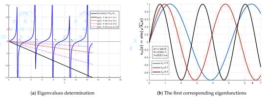
Figure 3. The eigenvalues determination and the corresponding eigenfunctions example (15).

• Case 1.2

The eigenfunctions corresponding to Case 1.2 are${\displaystyle v_n=cos\left(\sqrt{{\lambda }_n}x\right)}$with the eigenvalues determined by the equation${\displaystyle tan\left(\sqrt{{\lambda }_n}b\right)=\frac{b_1}{b_2\sqrt{{\lambda }_n}}}$.

• Case 2

The eigenfunctions corresponding to Case 2.1 are${\displaystyle v_n=\sqrt{{\lambda }_n}cos\left(\sqrt{{\lambda }_n}x\right)+sin\left(\sqrt{{\lambda }_n}x\right)}$with the eigenvalues determined by the equation${\displaystyle tan\left(\sqrt{{\lambda }_n}b\right)=-\frac{(b_1+b_2)\sqrt{{\lambda }_n}}{b_1-b_2\sqrt{{\lambda }_n}}}$. If b has the form${\displaystyle \frac{(2n+1)\pi }{2}·\frac{b_2}{b_1}}$, then${\displaystyle {\lambda }_n=\frac{b_1}{b_2}}$is the eigenvalue for the problem. In Figure 4a, the determination of the first eigenvalues is graphically presented as the roots of the function${\displaystyle tan\left(x\right)+\frac{(b_1+b_2)x}{b_{1}b-b_{2}x}}$with notation$x=\sqrt{{\lambda }_n}b$and in Figure 4b, the corresponding eigenfunctions are plotted.

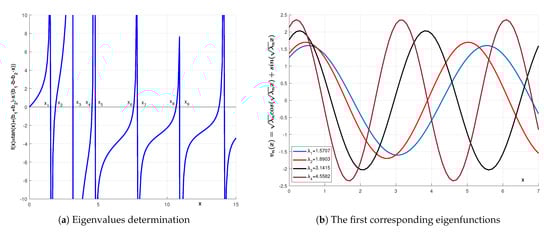
Figure 4. The eigenvalues determination and the corresponding eigenfunctions example 2.1.

For Case 2.2, the eigenfunctions are${\displaystyle v_n=\frac{\sqrt{{\lambda }_n}}{a_1}cos\left(\sqrt{{\lambda }_n}x\right)+sin\left(\sqrt{{\lambda }_n}\right)}$, and the eigenvalues are the solutions of the nonlinear equation${\displaystyle tan\left(\sqrt{{\lambda }_n}b\right)=\frac{(a_1-b_1)\sqrt{{\lambda }_n}}{a_1+\sqrt{{\lambda }_n}}}$.

Example 3. 

The conditions can be considerably weakened with respect to continuity and differentiability. In some cases, changes of variables, dependent and independent, may transform a problem from singular to regular; see [4].

For construction of the solutions, the Dirac function is used. Green’s function verifies${\displaystyle -\frac{d}{dx}\left[p\left(x\right)\frac{dG(x,y)}{dx}\right]+\rho \left(x\right)G(x,y)=\delta (x-y),}$and expresses the response under homogeneous boundary conditions to a forcing function consisting of a concentrated unit of inhomogeneity at$x=y.$

For the problem$-u^{″}\left(x\right)=\lambda u\left(x\right)+f\left(x\right)$in$(0,b)$;$u\left(0\right)=u\left(b\right)=0$,$\lambda =n^2$, the solution is${\displaystyle u\left(x\right)={\int }_0^{b}G(x,y)f\left(y\right)dy}$using the Green function

$$G(x,y)=\left\{\begin{array}{c}{\displaystyle \frac{sin\left(nx\right)sin\left(n\right(b-y\left)\right)}{nsin\left(nb\right)},0\le x<y}\hfill \\ {\displaystyle -\frac{sin\left(n\right(b-x\left)\right)sin\left(ny\right)}{nsin\left(nb\right)},y<x\le b.}\hfill \end{array}\right.$$

That leads to the representation

$${\displaystyle u\left(x\right)=\frac{sin\left(nx\right)}{nsin\left(nb\right)}{\int }_0^{x}sin\left(n(b-y)\right)f\left(y\right)dy-\frac{sin\left(n\right(b-x\left)\right)}{nsin\left(nb\right)}{\int }_x^{b}sin\left(ny\right)f\left(y\right)dy.}$$

Remark 4. 

Using the definition of the norm convergence, namely: “A sequence${\left({\phi }_n\right)}_n$in${\mathcal{L}}_s^2\left(I\right)$converges to$\phi \in {\mathcal{L}}_s^2\left(I\right)$if${\displaystyle \underset{n\to \infty }{lim}{∥{\phi }_n-\phi ∥}_s=0}$, i.e.,${\phi }_n\to \phi$in${\mathcal{L}}_s^2$norm”, some sequences${\delta }_n\left(x\right)$could be used instead of$\delta \left(x\right)$in order to obtain the Green function.

Starting from the definition$\delta (x-y)=\left\{\begin{array}{c}0,x\ne y\hfill \\ \infty ,x=y\hfill \end{array}\right.$and use some properties (see [6,9]):

δ is symmetric with${\displaystyle \delta \left(ax\right)=-\frac{1}{\left|a\right|}\delta \left(x\right)}$,${\displaystyle \delta \left(x\right)=\underset{n\to \infty }{lim}{\delta }_n\left(x\right)}$,${\displaystyle {\delta }_n\left(x\right)=\frac{n}{\sqrt{\pi }}{e}^{-n^2{x}^2}}$,${\displaystyle {\delta }_n\left(x\right)=\frac{{sin}^2\left(nx\right)}{n\pi x^2}}$or${\displaystyle {\delta }_n\left(x\right)=\frac{n}{\pi \left(1+n^2{x}^2\right)}}$, also

$${\displaystyle \delta \left(x^2-a^2\right)=\frac{1}{\left|2a\right|}[\delta (x+a)+\delta (x-a)]and{\int }_{-\infty }^{+\infty }f\left(y\right)\delta (x-y)dx=f\left(x\right).}$$

3. Variational RSL Problems

We define problem $P_1$ as follows:

$$\begin{array}{cc}\hfill -{\left(p{u}^{\prime }\right)}^{\prime }& +\rho u+\lambda su=f,\mathrm{on}(a,b)\hfill \end{array}$$

(16)

$$\begin{array}{cc}\hfill B_{1}u\left(a\right):& a_{1}u\left(a\right)+a_2{u}^{\prime }\left(a\right)=0\hfill \\ \hfill B_{2}u\left(b\right):& b_{1}u\left(b\right)+b_2{u}^{\prime }\left(b\right)=0\hfill \end{array}$$

(17)

and the set $V=\left\{v\in C^1\left([a,b]\right),v^{\prime }\mathrm{piecewise}\mathrm{continuous}\mathrm{on}[a,b],B_{1}v\left(a\right),B_{2}v\left(b\right)\mathrm{verified}\right\}$. For $v\in D\left(L\right)$, we have ${\displaystyle {\int }_a^{b}p{u}^{\prime }{v}^{\prime }dx+{\int }_a^b(\rho +\lambda s)uvdx={\int }_a^{b}fvdx,\forall v\in V}$ (see [10,11]).

Variational problem (VP${}_1$) associated to the problem $P1$ is as follows: find $u\in V$ such that $a(u,v)=\mathit{l}v$,$\forall v\in V$ with

$$\begin{array}{c}\hfill a(u,v)={\int }_a^{b}p{u}^{\prime }{v}^{\prime }+(\rho +\lambda s)uvdx,\forall u,v\in V;\mathit{l}v={\int }_a^{b}fvdx,\forall v\in V.\end{array}$$

(18)

The functional $F:V\to \mathbb{R}$, ${\displaystyle Fv=\frac{1}{2}a(u,v)-lv}$, $\forall v\in V$ expresses the difference between the internal elastic energy and the load potential.

Lemma 1. 

(i) 

$l:V\to \mathbb{R}$is linear;

(ii) 

Let$a:V\times V\to \mathbb{R}$with λ positive eigenvalue of RSL ($P_1$), then $a(u,v)$is bilinear functional, positive and symmetric.

Proof. 

(i) Let $v_1,v_2\in V$ and $\alpha ,\beta \in \mathbb{R}$, then ${\displaystyle \mathit{l}(\alpha v_1+\beta v_2)=\alpha \mathit{l}{v}_1+\beta \mathit{l}{v}_2}$ is the result that is obtained from the properties of the scalar product.

(ii) Let $u_1,u_2,v\in V$ and $\alpha ,\beta \in \mathbb{R}$ then

$$\begin{array}{cc}\hfill {\displaystyle a\left(\alpha u_1+\beta u_2,v\right)}& ={\int }_a^{b}p{\left(\alpha u_1+\beta u_2\right)}^{\prime }{v}^{\prime }+(\rho +\lambda s)\left(\alpha u_1+\beta u_2\right)vdx\hfill \\ \hfill & =\alpha {\int }_a^{b}p{u}_1^{\prime }{v}^{\prime }+(\rho +\lambda s)u_{1}vdx+\beta {\int }_a^{b}p{u}_2^{\prime }{v}^{\prime }+(\rho +\lambda s)u_{2}vdx\hfill \\ \hfill & =\alpha a\left(u_1,v\right)+\beta a\left(u_2,v\right)\hfill \end{array}$$

Let $u,v_1,v_2\in V$ and $\alpha ,\beta \in \mathbb{R}$, then

$$\begin{array}{cc}\hfill {\displaystyle a\left(u,\alpha v_1+\beta v_2\right)}& ={\int }_a^{b}p{u}^{\prime }{\left(\alpha v_1+\beta v_2\right)}^{\prime }+(\rho -\lambda s)u\left(\alpha v_1+\beta v_2\right)dx\hfill \\ \hfill & =\alpha {\int }_a^{b}p{u}^{\prime }{v}_1^{\prime }+(\rho +\lambda s)u{v}_{1}dx+\beta {\int }_a^{b}p{u}^{\prime }{v}_2+(\rho +\lambda s)u{v}_{2}dx\hfill \\ \hfill & =\alpha a\left(u,v_1\right)+\beta a\left(u,v_2\right)\hfill \end{array}$$

Let $u\in V$, then

$$\begin{array}{c}\hfill {\displaystyle a(u,u)={\int }_a^{b}p{\left(u^{\prime }\right)}^2+(\rho +\lambda s)u^{2}dx=p{\int }_a^b{\left(u^{\prime }\right)}^{2}dx+{\int }_a^b(\rho +\lambda s)u^{2}dx}\end{array}$$

The weight function $p\left(x\right)$ in $[a,b]$ is positive and in RSL($P_1$) conditions, $\rho +\lambda s$ is a positive function in $[a,b]$ accordingly $a(u,u)\ge 0$, $\forall u\in V$, and hence $a(·,·)$ is positive. Let $u,v\in V$, then

$$\begin{array}{c}\hfill a(u,v)={\int }_a^{b}p{u}^{\prime }{v}^{\prime }+(\rho +\lambda s)uvdx=a(v,u)\end{array}$$

Consequently, $a(·,·)$ is symmetric. □

Minimization problem ($M{P}_1$) associated to$\left(V{P}_1\right)$ is as follows.

Find $u\in V$ such that ${\displaystyle Fu=\underset{v\in V}{min}Fv}$ with

$$\begin{array}{c}\hfill {\displaystyle Fv=\frac{1}{2}{\int }_a^{b}p{\left(v^{\prime }\right)}^2+(\rho +\lambda s)v^{2}dx-{\int }_a^{b}fvdx}\end{array}$$

(19)

Theorem 1. 

(1) 

$u\in V$is the solution of$\left(V{P}_1\right)$if u is solution of$\left(M{P}_1\right)$;

(2) 

$u\in \mathcal{H}=C^1\left([a,b]\right)\cap C^2\left((a,b)\right)$, u solution of$\left(V{P}_1\right)$, then u solution of$\left(P_1\right)$.

Proof. 

(1) (i) Let $u\in V$ be the solution of $\left(V{P}_1\right)$, then $a(u,v)=lv,\forall v\in V$. For any $w\in V$, denoting $v=w-u\in V$, we have

$$\begin{array}{cc}\hfill {\displaystyle Fw-Fu}& =\frac{1}{2}a(u+v,u+v)-l(u+v)-Fu\hfill \\ \hfill & =Fu+Fv+a(u,v)-Fu=a(u,v)+F\left(v\right)\hfill \\ \hfill & =a(u,v)-lv+lu+F\left(v\right)=\frac{1}{2}a(v,v)\ge 0\hfill \end{array}$$

meaning that

$$\begin{array}{c}\hfill {\displaystyle Fu=\underset{w\in V}{min}Fw\mathrm{i}.\mathrm{e}.u\mathrm{solution}\mathrm{of}\left(M{P}_1\right)}\end{array}$$

(1) (ii) Let $u\in V$ be the solution of $\left(M{P}_1\right)$, then ${\displaystyle Fu=\underset{w\in V}{min}Fw}$; therefore, $Fw-Fu\ge 0,\forall w\in V$.

Using $w=u+tv$, $t\in \mathbb{R}$, one finds $F(u+tv)-Fu\ge 0,\forall t\in \mathbb{R}$ meaning

$$\begin{array}{c}\hfill {\displaystyle \frac{1}{2}a(u+tv,u+tv)-l(u+tv)-\frac{1}{2}a(u,u)+lu\ge 0,\forall t\in \mathbb{R},\forall u,v\in V}\end{array}$$

$$\begin{array}{c}\hfill {\displaystyle \frac{1}{2}a(u,u)+ta(u,v)+\frac{t^2}{2}a(v,v)-lu-tlv-\frac{1}{2}a(u,u)+lu\ge 0,\forall t\in \mathbb{R},\forall u,v\in V}\end{array}$$

$$\begin{array}{c}\hfill {\displaystyle \left[\frac{1}{2}a(v,v)\right]t^2+\left[a(u,v)-lv\right]t\ge 0\forall t\in \mathbb{R}}\end{array}$$

Using the positivity of the term $a(v,v)$, one finds

$$\begin{array}{c}\hfill {[a(u,v)-lv]}^2\le 0\Rightarrow a(u,v)=lv\forall v\in V\end{array}$$

meaning the u solution of $\left(V{P}_1\right)$.

(2) Let $u\in V\cap \mathcal{H}$ solution of $\left(V{P}_1\right)$, then

$$\begin{array}{cc}\hfill & {\int }_a^{b}p{u}^{\prime }{v}^{\prime }+(\rho +\lambda s)uvdx={\int }_a^{b}fvdx\hfill \\ \hfill & {\int }_a^{b}p{u}^{\prime }{v}^{\prime }dx+{\int }_a^b(\rho +\lambda s)uvdx={\int }_a^{b}fvdx\hfill \\ \hfill & {\left.\left(p{u}^{\prime }\right)v\right|}_a^b-{\int }_a^b{\left(p{u}^{\prime }\right)}^{\prime }vdx+{\int }_a^b(\rho +\lambda s)uvdx={\int }_a^{b}fvdx\hfill \\ \hfill & {\left.\left(p{u}^{\prime }\right)v\right|}_a^b+{\int }_a^b\left[-{\left(p{u}^{\prime }\right)}^{\prime }+(\rho +\lambda s)u-f\right]vdx=0,\forall v\in V\hfill \end{array}$$

In case of a self-adjoint operator for L, such as in the case of periodic or antiperiodic boundary conditions, we have

$$\begin{array}{c}\hfill {\left.\left(p{u}^{\prime }\right)v\right|}_a^b=p\left(b\right)u^{\prime }\left(b\right)v\left(b\right)-p\left(a\right)u^{\prime }\left(a\right)v\left(a\right)=0,\forall u,v\in V\end{array}$$

and one obtains ${\displaystyle {\int }_a^b\phi vdx=0,\forall v\in V}$ for $\phi \left(x\right)=-{\left(p{u}^{\prime }\right)}^{\prime }+(\rho +\lambda s)u\in C(a,b)$ that is $\phi \equiv 0$ over interval $(a,b)$.

This means that the u solution of $P_1$ also verifies the boundary conditions. □

The theorem proved above transfers the search space of the solution u of the problem $P_1$ to the search space for the solution of the problem $M{P}_1$, where the existence is ensured through the Lax–Milgram theorem for a coercive quadratic form, even more general from the Lions–Stampacchia theorem, where $a(·,·)$ is of a symmetric positive bilinear form.

4. Variational Approaches for VP of RSL

4.1. Nehari Variational Method

Let $u\in C^2\left([a,b]\right)$ and $F:[a,b]\times C^2\left([a,b]\right)\times C\left([a,b]\right)\to [a,b]$ be a function that has continuous second-order derivatives with respect to all of its arguments. According to the Euler–Lagrange variational principle, a necessary condition for the functional

$$\begin{array}{c}\hfill {\displaystyle J\left(u\right)={\int }_a^{b}F\left(x,u,u^{\prime }\right)dx,}\end{array}$$

(20)

to be stationary at u is that u is a solution of the Euler–Lagrange equation (see [3])

$$\begin{array}{c}\hfill \frac{\partial F}{\partial u}-\frac{d}{dx}\left(\frac{\partial F}{\partial u^{\prime }}\right)=0,a\le x\le b\end{array}$$

(21)

with the Dirichlet conditions $u\left(a\right)=A\mathrm{and}u\left(b\right)=B.$

For a nonlinear RSL problem,

$$\begin{array}{c}\hfill -u^{\prime }=f(x,u^2),f\in \mathcal{H},x\in (a,b)=I;u\left(a\right)=A\mathrm{and}u\left(b\right)=B,\end{array}$$

(22)

for $\mathcal{H}=\left\{f\in C\left(\right[a,b]\times [0,\infty \left]\right)|f\mathrm{verifies}\left(\mathrm{ip}1\right),\left(\mathrm{ip}2\right)\mathrm{and}\mathrm{boundary}\mathrm{conditions}\right\}$.

$$\begin{array}{cc}\hfill \left(\mathrm{ip}1\right):& f(x,y)>0\mathrm{for}y>0\hfill \\ \hfill \left(\mathrm{ip}2\right):& \exists \nu ,y^{-\nu }f(x,y)\mathrm{is}\mathrm{a}\mathrm{non}-\mathrm{decreasing}\mathrm{function}\mathrm{of}y\in [0,\infty )\hfill \end{array}$$

For the problem (22), looking for the extremum value of the functional

$$\begin{array}{c}\hfill {\displaystyle J\left(u\right)={\int }_a^b\left[{\left(u^{\prime }\right)}^2-{\int }_0^{u^2\left(x\right)}\left(f(x,y)dy\right)\right]dx,}\end{array}$$

(23)

for the set $V_{a,b}=\left\{u|u\in C\left([a,b]\right),u^{\prime }\mathrm{piecewise}\mathrm{continuous}\mathrm{in}[a,b],u\left(a\right)=u\left(b\right)=0\right\}$ the functional $J\left(u\right)$ is not bounded. Using the Nehari method, a new condition on the function f and u is imposed:

$$\begin{array}{c}\hfill {\displaystyle {\int }_a^b{\left(u^{\prime }\right)}^{2}dx={\int }_a^b{u}^{2}f(x,u^2)dx,}\end{array}$$

(24)

which is satisfied by the solutions of (22).

Let us consider the set ${\mathcal{V}}_{a,b}=\left\{u|u\in V_{a,b}\mathrm{verifies}\left(24\right)\right\}$. For I given, let ${\displaystyle \mu (a,b)=\underset{u\in V}{inf}J\left(u\right)}$. Then $\exists u\in {\mathcal{V}}_{a,b}$ such that $J\left(u\right)=\mu (a,b)$ and also (see [12]), for $u\in {\mathcal{V}}_{a,b}$ with $J\left(u\right)=\mu (a,b)$, $w=\left|u\right|\in {\mathcal{V}}_{a,b}$ is a positive solution of (22).

The function $\mu (a,b)$ is continuous with respect to both arguments and

$${\displaystyle \mu (a,b)=\underset{c<d\in [a,b]}{inf}\mu (c,d)\mathrm{with}\underset{b\to a}{lim}\mu (a,b)=\infty .}$$

(25)

Remark 5. 

For a partition${\Delta }_n:a=x_0<x_1<\cdots <x_{n-1}<x_n=b$of the interval I, over each subinterval$[x_i;x_{i+1}]$, consider$u_i\in {\mathcal{V}}_{x_i,x_{i+1}}$normalized with the Nehari condition and

$$\begin{array}{cc}For& x\in [x_i;x_{i+1}]:u\left(x\right)={(-1)}^i\left|u_i\left(x\right)\right|,J\left(u\right)={\mu }_{n-1}(x_1,x_2,\cdots ,x_{n-1})\end{array}$$

(26)

$$\begin{array}{cc}For& {\displaystyle {\Delta }_n\mathrm{given}:{\mu }_{n-1}(x_1,x_2,\cdots ,x_{n-1})=\sum _{i=1}^n\mu (x_{i-1},x_i),}\hspace{1em}\hspace{1em}\hspace{1em}\hspace{1em}\hspace{1em}\hspace{1em}\end{array}$$

(27)

then the solution$u\left(x\right)$is in$V_{a,b}$and is vanishing$n-1$times over interval I. Additionally, if$|u_k^{\prime }\left(x_k\right)|\ne |u_{k+1}^{\prime }\left(x_k\right)|$then${\mu }_{n-1}(x_1,x_2,\cdots ,x_{n-1})$is not a minimum of${\displaystyle \sum _{i=1}^n\mu (x_{i-1},x_i)}$.

4.2. Variational Estimations for RSL

In the following, two variational estimation methods are presented, the shooting method and bisection method, consisting in solving the variational equations associated to the problem given.

• Shooting method:

$$\left(P_2\right)\left\{\begin{array}{c}-{\left(p{u}^{\prime }\right)}^{\prime }+(q+\lambda s)u=0,x\in [a,b]\hfill \\ u\left(a\right)=0,u\left(b\right)=0\hfill \end{array}\right.$$

(28)

For $\lambda$ eigenvalue and $u_{\lambda }\left(x\right)$, the corresponding eigenfunction $u_{\lambda }\left(a\right)\ne 0$ and ${\displaystyle y=\frac{u_{\lambda }}{u_{\lambda }^{\prime }\left(a\right)}}$ is the normalized eigenfunction with $y^{\prime }\left(a\right)=1$, which is the solution for the variational equation associated to (28) with the initial value conditions:

$$\left(VIP\right)\left\{\begin{array}{c}-{\left(p{y}^{\prime }\right)}^{\prime }+(q+\lambda s)y=0,x\in [a,b]\hfill \\ y\left(a\right)=0,y^{\prime }\left(a\right)=1\hfill \end{array}\right.$$

(29)

with $y\left(b\right)=0$ (see [4]).

Algorithm of the shooting method:

Step 1

Determine an interval of an eigenvalue and make a guess;

Step 2

Solve VIP ($P_2$) and find the eigenfunction $u=u_{\lambda }\left(x\right)$;

Step 3

If $u_{\lambda }\left(b\right)=0$ or $\left|u_{\lambda }\left(b\right)\right|<\epsilon$ given, then Stop.

Else, find $\lambda$ the root of $u_{\lambda }\left(b\right)=0$ in a given interval and update $\lambda$.

GO TO Step 1.

• Bisection method

For SL eigenvalue problem $\left(P_3\right)$ with functions and constants satisfying RSL assumptions (1)–(4):

$$\left(P_3\right)\left\{\begin{array}{c}-{\left(p{u}^{\prime }\right)}^{\prime }+(q+\lambda s)u=0,x\in [a,b]\hfill \\ B_{1}u\left(a\right):a_{1}u\left(a\right)+a_2{u}^{\prime }\left(a\right)=0\hfill \\ B_{2}u\left(b\right):b_{1}u\left(b\right)+b_2{u}^{\prime }\left(b\right)=0\hfill \end{array}\right.$$

(30)

the related variational initial value problem $VI{P}_3$ is

$$\left(VI{P}_3\right)\left\{\begin{array}{c}-{\left(p{u}^{\prime }\right)}^{\prime }+(q+\lambda s)u=0,,x\in [a,b]\hfill \\ {\displaystyle u\left(a\right)=-\frac{a_2}{\sqrt{a_1^2+a_2^2}};u^{\prime }\left(a\right)=\frac{a_1}{\sqrt{a_1^2+a_2^2}}}\hfill \end{array}\right.$$

(31)

For the eigenvalue $\lambda$ denoting $u_{\lambda }$, the corresponding eigenfunction has $u_{\lambda }\left(0\right)\ne 0$, and $y=u_{\lambda }$ is the normalized $u_{\lambda }$ eigenfunction such that $a_{1}y\left(a\right)+a_2{y}^{\prime }\left(a\right)=0$. In this case, $\lambda$ is the eigenvalue for $P_3$ if $F\left(\lambda \right):=B_{2}y\left(b\right)=b_{1}y\left(b\right)+b_2{y}^{\prime }\left(b\right)=0$.

The function ${\displaystyle w_{\lambda }\left(x\right)=\frac{\partial u_{\lambda }}{\partial \lambda }}$ satisfies the variational initial value problem $\left(VIV{P}_3\right)$.

$$\left(VIV{P}_3\right)\left\{\begin{array}{c}-{\left(p{w}^{\prime }\right)}^{\prime }+(q+\lambda s)w+sw=0\hfill \\ w\left(a\right)=0,w^{\prime }\left(a\right)=0\hfill \end{array}\right.$$

(32)

and $F\left(\lambda \right)=b_1{u}_{\lambda }\left(b\right)+b_2{u}_{\lambda }^{\prime }\left(b\right)$ is a continuously differentiable function on $\lambda$ with $F^{\prime }\left(\lambda \right)=b_1{w}_{\lambda }\left(b\right)+b_2{w}_{\lambda }^{\prime }\left(b\right)\ne 0$.

Remark 6. 

Under RSL assumptions (1)–(4), if λ is the eigenvalue of$\left(P_3\right)$and$y=u_{\lambda }$is the corresponding normalized eigenfunction, then there exists$({\lambda }_{inf},{\lambda }_{sup})$containing λ such that$F\left({\lambda }_{inf}\right)F\left({\lambda }_{sup}\right)<0$and the approximate sequence${\left({\lambda }_n\right)}_n$is convergent,${\lambda }_n\to \lambda$and$y_n=u_{{\lambda }_n}$are the corresponding eigenfunctions obtained by solving$\left(VIV{P}_3\right)$such that$y_n\to y$and$y_n^{\prime }\to y^{\prime }$.

For instance, the solution of the problem

$$\left(E{P}_3\right)\left\{\begin{array}{c}-{\left(p\left(x\right)u^{\prime }\right)}^{\prime }+\rho u\left(x\right)=f\left(x\right),x\in (0,1)\hfill \\ u\left(0\right)=0,u\left(1\right)=0\hfill \end{array}\right.$$

(33)

with $p,\rho ,f\in C\left(\right[0,1\left]\right)$ verifying (RSL) conditions (1)–(4) is obtained solving the associated

$$(VI-E{P}_3)\left\{\begin{array}{c}-{\left(p{y}^{\prime }\right)}^{\prime }+\rho y=f\left(x\right),x\in (0,1)\hfill \\ y\left(0\right)=0,y\left(1\right)=s\hfill \end{array}\right.$$

(34)

The solution of $\left(E{P}_3\right)$ is determined such that $u_s\left(x\right)=u_p\left(x\right)+sv\left(x\right)$ with $u_s\left(1\right)=0$ and $u_p$ is a particular solution of $Ly=f$ and v satisfies

$$Lv=0,v\left(0\right)=0;v^{\prime }\left(0\right)=1.$$

4.3. Iterative Variational Methods for RSL

Among analytical estimation methods, the variational iteration method (VIM or He’s methods, see [13]) and homotopy perturbation method (HPM) (see [14,15]) are considered to find approximations for the nonlinear equation

$$\begin{array}{c}\hfill Lu+\lambda s\left(x\right)u=f(x,u,u^{\prime }),x\in (a,b)=I,\lambda \in \mathbb{R},\end{array}$$

(35)

under different boundary conditions (Dirichlet, Neumann or general case $B_{1}u\left(a\right),B_{2}u\left(b\right))$.

4.3.1. He’s Variational Method (VIM)

For the nonlinear Equation (35), we define N as the nonlinear operator such that (35) becomes

$$\begin{array}{c}\hfill Lu+Nu=g\left(x\right),x\in (a,b)=I,\end{array}$$

(36)

and the correction functional for the general Lagrange multiplier method is

$$\begin{array}{c}\hfill {\displaystyle u_{n+1}\left(x\right)=u_n\left(x\right)+{\int }_0^x\mu \left(t,x,\lambda \right)\left[L{u}_n\left(t\right)+N{\tilde{u}}_n\left(t\right)-g\left(t\right)\right]dt,}\end{array}$$

(37)

with ${\tilde{u}}_n$ considered as restricted variation, $\delta {\tilde{u}}_n=0$, and $\mu \left(t,x,\lambda \right)$ a Lagrange multiplier determined through the calculus of variations from (37); see [10,16].

$$\begin{array}{c}\hfill {\displaystyle \delta u_{n+1}\left(x\right)=\delta u_n\left(x\right)+\delta {\int }_0^x\mu \left(t,x,\lambda \right)\left[L{u}_n\left(t\right)+N{\tilde{u}}_n\left(t\right)-g\left(t\right)\right]dt.}\end{array}$$

(38)

4.3.2. Homotopy Perturbation Method (HPM)

For the nonlinear Equation (35) we define the operators $\mathcal{L}$ and N for $q\in [0,1]$

$$\begin{array}{cc}\mathcal{L}[\Phi (x,q\left)\right]& {\displaystyle =-\frac{d}{dx}\left[p\left(x\right)\frac{d}{dx}\Phi (x,q)\right],}\hspace{1em}\hspace{1em}\hspace{1em}\hspace{1em}\hspace{1em}\hspace{1em}\hspace{1em}\hspace{1em}\hspace{1em}\hspace{1em}\hspace{1em}\hspace{1em}\hspace{1em}\hspace{1em}\hspace{1em}\hspace{1em}\hspace{1em}\end{array}$$

(39)

$$\begin{array}{cc}N[\Phi (x,q\left)\right]& {\displaystyle =-\frac{d}{dx}\left[p\left(x\right)\frac{d}{dx}\Phi (x,q)\right]+(\rho +\lambda s)\left(x\right)\Phi (x,q)-f(x,\Phi (x,q),{\Phi }_x(x,q)),}\end{array}$$

(40)

given by the maximum order of derivation from the equation and by the form of the equation; see [14,17]. We write the zero-order equation associated with the initial equation:

$$\begin{array}{c}\hfill (1-q)\mathcal{L}\left[\Phi (x,q)-u_0\left(x\right)\right]=hqN[\Phi (x,q)]\end{array}$$

(41)

with h as a nonzero parameter, $u_0$ as a first analytical approximation of the function u with conditions

$$\begin{array}{c}\hfill \Phi (x,0)=u_0\left(x\right);\Phi (x,1)=u\left(x\right),x\in [a,b].\end{array}$$

(42)

where $u_0$ is a initial function that verifies the boundary conditions $B_{1}u\left(a\right):a_{1}u\left(a\right)+a_2{u}^{\prime }\left(a\right)=0,B_{2}u\left(b\right):b_{1}u\left(b\right)+b_2{u}^{\prime }\left(b\right)=0$ could be obtained from polynomial approximation developing the function f.

We develop $\Phi (x,q)$ by a Taylor series in the vicinity of the origin in relation to the second variable

$$\begin{array}{c}\hfill \Phi (x,q)=u_0\left(x\right)+\sum _1^{\infty }{u}_m\left(x\right)q^m;u_m\left(x\right)={\left.\frac{1}{m!}\frac{{\partial }^m\Phi }{\partial x^m}(x,q)\right|}_{q=0}\end{array}$$

(43)

A good choice for h (in relation to the error obtained compared to the initial equation) leads to $u\left(x\right)=u_0\left(x\right)+{\sum }_{m=1}^{\infty }{u}_m\left(x\right)$.

The equation of order m:

• case $m=1\to \mathcal{L}\left[u_m\left(x\right)\right]=hN\left[u_{m-1}\right]$
• case $m\ge 2\to \mathcal{L}\left[f_m\left(x\right)-f_{m-1}\left(x\right)\right]=hN\left[u_{m-1}\right]$

with boundary conditions $B_1{u}_m\left(a\right),B_2{u}_m\left(b\right).$

For the approximation of order 1, we have

$$\begin{array}{c}\hfill {\displaystyle -{\left[p\left(x\right)u_1^{\prime }\left(x\right)\right]}^{\prime }=h\underset{{\epsilon }_0\left(x\right)}{\underbrace{\left\{{\displaystyle -{\left[p\left(x\right)u_0^{\prime }\left(x\right)\right]}^{\prime }+(\rho \left(x\right)+\lambda s\left(x\right))u_0\left(x\right)-f(x,u_0\left(x\right),u_0^{\prime }\left(x\right))}\right\}}}}\end{array}$$

(44)

with ${\epsilon }_1(x,h)=N\left[u_1\left(x\right)\right].$

The parameter h at step 1 is chosen such that the value of ${max}_{x\in I}\left|{\epsilon }_1(x,h)\right|$ is the smallest possible and becomes the next value of ${\epsilon }_1$, but also could be taken as $h=1$. Iteratively, for $m\ge 2$

$$\begin{array}{c}\hfill L{u}_m+\lambda s\left(x\right)u_m=f(x,u_{m-1},u_{m-1}^{\prime }),x\in I;B_1{u}_m\left(a\right),B_2{u}_m\left(b\right)\end{array}$$

(45)

with start condition $u_0$ being known and stop condition ${max}_x\left|u_m-u_{m-1}\right|<ϵ$.

4.3.3. Applications

Let us consider a nonlinear RSL, such as the following problem:

$$\begin{array}{c}\hfill -u^{″}\left(x\right)+\lambda u\left(x\right)=f\left(x,u,u^{\prime }\right),x\in [0,b];B_{1}u\left(0\right),B_{2}u\left(b\right).\end{array}$$

(46)

The corresponding correction functional (37) to the problem (46) for the variational iteration method leads to the general Lagrange multiplier

$$\begin{array}{cc}\mathrm{for}\lambda >0,& {\displaystyle \mu \left(t,x,\lambda \right)=\frac{1}{2\alpha }\left(e^{\alpha (t-x)}-e^{\alpha (x-t)}\right)=\frac{1}{\alpha }sinh\alpha (t-x),\alpha =\sqrt{\lambda }}\end{array}$$

(47)

$$\begin{array}{cc}\mathrm{for}\lambda <0,& {\displaystyle \mu \left(t,x,\lambda \right)=-\frac{1}{\alpha }sin\alpha (t-x),\alpha =\sqrt{-\lambda }}\hspace{1em}\hspace{1em}\hspace{1em}\hspace{1em}\hspace{1em}\hspace{1em}\hspace{1em}\hspace{1em}\hspace{1em}\end{array}$$

(48)

and for $f\left(x,u,u^{\prime }\right)=g\left(x\right)$, one finds

$$\begin{array}{cc}\hfill u_{n+1}\left(x\right)=& {\displaystyle u_n\left(x\right)+\frac{1}{\alpha }{\int }_0^{x}sinh\alpha (t-x)\left[-u_n^{″}\left(t\right)+{\alpha }^2{u}_n\left(t\right)-g\left(t\right)\right]dt,\lambda >0,}\hfill \end{array}$$

(49)

$$\begin{array}{cc}\hfill u_{n+1}\left(x\right)=& {\displaystyle u_n\left(x\right)-\frac{1}{\alpha }{\int }_0^{x}sin\alpha (t-x)\left[-u_n^{″}\left(t\right)+{\alpha }^2{u}_n\left(t\right)-g\left(t\right)\right]dt,\lambda <0}\hfill \end{array}$$

(50)

with $u_0\left(x\right)=A+Bx$. Particularly, for $g\left(x\right)=x$, the first step leads to

$$\begin{array}{cc}\hfill u_1\left(x\right)=& {\displaystyle u_0\left(x\right)+\frac{1}{\alpha }{\int }_0^{x}sinh\alpha (t-x)\left[\lambda A+(\lambda B-1)t\right]dt,\lambda ={\alpha }^2,}\hfill \end{array}$$

(51)

$$\begin{array}{cc}\hfill u_1\left(x\right)=& {\displaystyle u_0\left(x\right)-\frac{1}{\alpha }{\int }_0^{x}sin\alpha (t-x)\left[\lambda A+(\lambda B-1)t\right]dt,\lambda =-{\alpha }^2}\hfill \end{array}$$

(52)

from where

$$\begin{array}{cc}{u}_1\left(x\right)=& 2A+2Bx+\frac{{\alpha }^{2}B-1}{{\alpha }^3}sinh\left(\alpha x\right)-Acosh\left(\alpha x\right)-\frac{x}{{\alpha }^2},\lambda ={\alpha }^2,\end{array}$$

(53)

$$\begin{array}{cc}{u}_1\left(x\right)=& 2A+\frac{{\alpha }^{2}B-1}{{\alpha }^3}sin\left(\alpha x\right)-Acos\left(\alpha x\right)+\frac{x}{{\alpha }^2},\lambda =-{\alpha }^2,\hspace{1em}\hspace{1em}\hspace{1em}\end{array}$$

(54)

For $n>1$, we have

$$\begin{array}{cc}{u}_{n+1}\left(x\right)=& {\displaystyle u_n\left(x\right)+\frac{1}{\alpha }{\int }_0^{x}sinh\alpha (t-x)\left[-u_n^{″}\left(t\right)+{\alpha }^2{u}_n\left(t\right)-t\right]dt,\lambda >0,}\end{array}$$

(55)

$$\begin{array}{cc}{u}_{n+1}\left(x\right)=& {\displaystyle u_n\left(x\right)-\frac{1}{\alpha }{\int }_0^{x}sin\alpha (t-x)\left[-u_n^{″}\left(t\right)+{\alpha }^2{u}_n\left(t\right)-t\right]dt,\lambda <0}\hspace{1em}\end{array}$$

(56)

Constants A and B are determined from the boundary condition imposed to the last function $u_n$ computed, and for $u\left(x\right)=u_n\left(x\right)$, boundary conditions are imposed, resulting in a system for the constants $A,B$. Thus, the solution of the problem is obtained.

In the case of using HPM, Equation (44), with $\lambda ={\alpha }^2$, for the first step becomes

$$\begin{array}{c}\hfill {\displaystyle -u_1^{″}\left(x\right)=h\left({\displaystyle -u_0^{″}\left(x\right)+\lambda u_0\left(x\right)-x}\right)=h{\epsilon }_0\left(x\right)}\end{array}$$

(57)

and for case $m\ge 2$

$$\begin{array}{c}\hfill -\left[{\displaystyle u_m^{″}-u_{m-1}^{″}}\right]\left(x\right)=h\left({\displaystyle -u_{m-1}^{″}\left(x\right)+\lambda u_{m-1}\left(x\right)-x}\right)={\epsilon }_m(x,h).\end{array}$$

(58)

One obtains

$$\begin{array}{c}{u}_1\left(x\right)=-h\left(\frac{\lambda A{x}^2}{2}+\frac{(\lambda B-1)x^3}{3}\right),\hspace{1em}\hspace{1em}\hspace{1em}\hspace{1em}\hspace{1em}\hspace{1em}\hspace{1em}\hspace{1em}\hspace{1em}\hspace{1em}\hspace{1em}\hspace{1em}\hspace{1em}\hspace{1em}\hspace{1em}\hspace{1em}\hspace{1em}\end{array}$$

(59)

$$\begin{array}{c}{u}_2^{″}=h(1-h)(\lambda A+(\lambda B-1)x)+hx-h^2\left(\frac{{\lambda }^{2}A{x}^2}{2}+\lambda \frac{(\lambda B-1)x^3}{3}\right)=-{\epsilon }_1(x,h).\end{array}$$

(60)

from where

$$\begin{array}{c}\hfill u_2=h(1-h)(\lambda A\frac{x^2}{2}+(\lambda B-1)\frac{x^3}{6})+h\frac{x^3}{6}-h^2\left(\frac{{\lambda }^{2}A{x}^4}{24}+\lambda \frac{(\lambda B-1)x^5}{603}\right).\end{array}$$

(61)

The solution will be $u\left(x\right)=u_0\left(x\right)+u_1\left(x\right)+u_2\left(x\right)+\dots$.

Additionally, if we consider the nonlinearity in (46) through function $f\left(x,u,u^{\prime }\right)=g\left(x\right)u$, that is, for $g\left(x\right)=-x^2$, $x\in (-\mathit{l},\mathit{l})$ we are in the harmonic oscillator case ($\lambda <0$), then the following correction functional appears

$$\begin{array}{cc}\hfill u_{n+1}\left(x\right)=& {\displaystyle u_n\left(x\right)+\frac{1}{\alpha }{\int }_0^{x}sinh\alpha (t-x)\left[-u_n^{″}\left(t\right)+({\alpha }^2-g\left(t\right))u_n\left(t\right)\right]dt,\lambda >0,}\hfill \end{array}$$

(62)

$$\begin{array}{cc}\hfill u_{n+1}\left(x\right)=& {\displaystyle u_n\left(x\right)-\frac{1}{\alpha }{\int }_0^{x}sin\alpha (t-x)\left[-u_n^{″}\left(t\right)+({\alpha }^2-g\left(t\right))u_n\left(t\right)\right]dt,\lambda <0}\hfill \end{array}$$

(63)

as an eigenfunction of the equation Hermite polynomials appears.

For $B_{1}u(-\mathit{l}):u(-\mathit{l})=0;B_{2}u(-\mathit{l}):u\left(\mathit{l}\right)=0$ and ($\lambda <0$)

$$\begin{array}{cc}\hfill u_1\left(x\right)=& {\displaystyle A+Bx-\frac{1}{\alpha }{\int }_0^{x}sin\alpha (t-x)\left[t^2(A+Bt)+{\alpha }^2(A+Bt)\right]dt,}\hfill \end{array}$$

(64)

$$\begin{array}{cc}\hfill u_{n+1}\left(x\right)=& {\displaystyle u_n\left(x\right)-\frac{1}{\alpha }{\int }_0^{x}sin\alpha (t-x)\left[-u_n^{″}\left(t\right)+({\alpha }^2+t^2)u_n\left(t\right)\right]dt,}\hfill \end{array}$$

(65)

$$\begin{array}{c}\hfill {\displaystyle -u_1^{″}\left(x\right)=h\left({\displaystyle -u_0^{″}\left(x\right)+(x^2+{\alpha }^2)u_0\left(x\right)}\right)=h{\epsilon }_0\left(x\right)}\end{array}$$

(66)

and for case $m\ge 2$

$$\begin{array}{c}\hfill -\left[{\displaystyle u_m^{″}-u_{m-1}^{″}}\right]\left(x\right)=h\left({\displaystyle -u_{m-1}^{″}\left(x\right)+(x^2+{\alpha }^2)u_{m-1}\left(x\right)}\right)={\epsilon }_m(x,h).\end{array}$$

(67)

The two methods are fast convergent methods.

Variational iteration methods, such as VIM and HPM, could be used also for nonlinear propagation problems in which the temporal variable is considered, for example, for the coupled pseudo-parabolic equation, or the one-dimensional coupled Burgers equation numerically studied in [18]. The nonlinear coupled Burgers equations are also studied in [19] as an application of EOHAM (extension optimal homotopy asymptotic method) in which homotopy is combined with perturbation techniques. The Newell–Whitehead–Segel equation (NWSE) was also studied using the VIM technique and He’s polynomials [20].

5. Conclusions

In the first part of the paper, definitions and results are presented connected to regular and singular Sturm–Liouville problems. Some types of direct singular SLPs were solved in [5,21] and a study of the inverse SLP algorithm was made. We defined in a different manner the SLP, and different boundary conditions were considered. All the figures were made using Matlab codes, the academic versions.

In the core of the paper, the variational formulation (VP) through a bilinear functional positive and symmetric is made. The minimization problem (MP) is also outlined through the functional of energy, and the equivalence of the formulations under some conditions imposed for RSL problems is proved.

Variational estimations are in the final part of the paper through the construction of the solution trough variational equations associated to the problem, such as the shooting method and bisection method, or using a sequential analytical approximate solution that is constructed according to the accuracy established. Here, we present He’s variational method and the homotopy method. In the closing part, a is taken into account and the sequentiality of the transition from one step to another is specified for both methods. Al-Khaled et al. (see [22]) solve numerically a SLP using the general Sinc–Galerkin and Newton method but for different types of boundary conditions. In the paper, He’s method, the Adomian method and Lagrange multiplier for special ODEs were given in detail, numerical results being obtained for Duffing and Titchmarch equations. We considered our applications the interval $(0,b)$ and general conditions $B_{1}u\left(0\right),B_{2}u\left(b\right)$ for a linear and a nonlinear case of $f\left(x,u,u^{\prime }\right)$.

In [23] spectral problems of the nonlocal SLP with an integral $B_{2}u\left(b\right)$ were studied. Kernel of the operator, properties of the first eigenvalue and oscillation properties of eigenfunctions to the nonlocal problem were expressed. Additionally, the solution of the Cauchy problem for the SL equation on a star graph was constructed in [24].

For fractional differential equations, VIM could also be a very powerful instrument, in which Equations (36) and (37) are written using the Caputo fractional derivative, see [25]. This is our intention for the new study.

Nonlinear RSL problems could appear in the case of non-Newtonian fluid flows. Variational estimation methods are efficient techniques for finding analytical approximate solutions for a class of problems and also for optimal problems when looking for a minimum, using the functional of energy.

References

- Dautray, R.; Lions, J.L. Mathematical Analysis and Numerical Methods for Science and Technology; Springer: Berlin/Heidelberg, Germany, 2000. [Google Scholar]
- Fowler, A.C. Mathematical Models in the Applied Sciences; Cambridge University Press: Cambridge, UK, 1997. [Google Scholar]
- Tyn Myint-U, T.; Debnath, L. Linear Partial Differential Equations for Scientists and Engineers, 4th ed.; Springer: Berlin, Germany, 2007; ISBN 0-8176-4393-1. [Google Scholar]
- Guenther, R.B.; Lee, J.W. Sturm-Liouville Problems. Theory and Numerical Implementation; CRC Press: Boca Raton, FL, USA, 2019; ISBN 9781138345430. [Google Scholar]
- Perera, U.; Böckmann, C. Solutions of Sturm-Liouville Problems. Mathematics 2020, 8, 2074. [Google Scholar] [CrossRef]
- Hassana, A.A. Green’s Function Solution of Non-Homogenous Regular Sturm-Liouville Problem. J. Appl. Comput. Math. 2017, 6, 362. [Google Scholar] [CrossRef]
- Klimek, M. Spectrum of Fractional and Fractional Prabhakar Sturm–Liouville Problems with Homogeneous Dirichlet Boundary Conditions. Symmetry 2021, 13, 2265. [Google Scholar] [CrossRef]
- Razdan, A.K.; Ravichandran, V. Fundamentals of Partial Differential Equations; Springer: Singapore, 2022. [Google Scholar] [CrossRef]
- Guo, H.; Qi, J. Sturm–Liouville Problems Involving Distribution Weights and an Application to Optimal Problems. J. Optim. Theory Appl. 2020, 184, 842–857. [Google Scholar] [CrossRef]
- Altintan, D.; Ugur, O. Variational iteration method for Sturm-Liouville differential equations. Comput. Math. Appl. 2008, 58, 322–328. [Google Scholar] [CrossRef]
- Johnson, C. Numerical Solution of Partial Differential Equations by the Finite Element Method; Cambridge University Press: Cambridge, UK, 1987; ISBN 0521345146. [Google Scholar]
- Chen, C.N. A survey of nonlinear Sturm-Liouville equations. In Sturm-Liouville Theory: Past and Present; Amrein, W.O., Hinz, A.M., Eds.; Pearson D.P.: Basel, Switzerland, 2005; pp. 201–216. [Google Scholar]
- He, J.H.; Wu, X.H. Variational iteration method: New development and applications. Comput. Math. Appl. 2007, 54, 881–894. [Google Scholar] [CrossRef]
- Hayat, T.; Khan, M.; Ayub, M. On the non-linear flows with slip boundary condition. Z. Angew. Math. Phys. 2005, 56, 1012–1029. [Google Scholar] [CrossRef]
- Yusufoglu, E.; Bekir, A. On the extended tanh method applications of nonlinear equations. Int. J. Nonlinear Sci. 2007, 4, 10–16. [Google Scholar]
- Neamaty, A.; Darzi, R. Comparison between the Variational Iteration Method and the Homotopy Perturbation Method for the Sturm-Liouville Differential Equation. Bound. Value Probl. 2010, 2010, 317369. [Google Scholar] [CrossRef]
- Zhang, T.-T.; Jia, L.; Wang, Z.-C. Analytic Solution for Steady Slip Flow between Parallel Plates with Micro-Scale Spacing. Chin. Phys. Lett. 2008, 25, 180. [Google Scholar] [CrossRef]
- Nadeem, M.; Yao, S. Solving system of partial differential equations using variational iteration method with He’s polynomials. Int. J. Math. Comput. Sci. 2019, 19, 203–211. [Google Scholar] [CrossRef]
- Fiza, M.; Chohan, F.; Ullah, H.; Islam, S.; Bushnaq, S. An extension of the optimal homotopy asymptotic method with applications to nonlinear coupled partial differential equations. J. Math. Comput. Sci. 2019, 19, 218–229. [Google Scholar] [CrossRef]
- Nadeem, M.; Yao, S.; Parveen, N. Solution of Newell-Whitehead-Segel equation by variational iteration method with He’s polynomials. J. Math. Comput. Sci. 2020, 20, 21–29. [Google Scholar] [CrossRef]
- Herron, I.H. Solving singular boundary value problems for ordinary differential equations. Caribb. J. Math. Comput. Sci. 2013, 15, 1–30. [Google Scholar]
- Al-Khaled, K.; Hazaimeh, A. Comparison Methods for Solving Non-Linear Sturm–Liouville Eigenvalues Problems. Symmetry 2020, 12, 1179. [Google Scholar] [CrossRef]
- Liu, Z.; Qi, J. The Properties of Eigenvalues and Eigenfunctions for Nonlocal Sturm–Liouville Problems. Symmetry 2021, 13, 820. [Google Scholar] [CrossRef]
- Kanguzhin, B.; Aimal Rasa, G.H.; Kaiyrbek, Z. Identification of the Domain of the Sturm–Liouville Operator on a Star Graph. Symmetry 2021, 13, 1210. [Google Scholar] [CrossRef]
- Nagdy, A.; Hashem, K.H. Numerical solutions of nonlinear fractional differential equations by variational iteration method. J. Nonlinear Sci. Appl. 2021, 14, 54–62. [Google Scholar] [CrossRef]
Publisher’s Note: MDPI stays neutral with regard to jurisdictional claims in published maps and institutional affiliations. |
© 2022 by the authors. Licensee MDPI, Basel, Switzerland. This article is an open access article distributed under the terms and conditions of the Creative Commons Attribution (CC BY) license (https://creativecommons.org/licenses/by/4.0/).