Convergence of Uniformity Criteria and the Application in Numerical Integration

Abstract

Quasi-Monte Carlo (QMC) methods have been successfully used for the estimation of numerical integrations arising in many applications. In most QMC methods, low-discrepancy sequences have been used, such as digital nets and lattice rules. In this paper, we derive the convergence rates of order of some improved discrepancies, such as centered $L_2$-discrepancy, wrap-around $L_2$-discrepancy, and mixture discrepancy, and propose a randomized QMC method based on a uniform design constructed by the mixture discrepancy and Baker’s transformation. Moreover, the numerical results show that the proposed method has better approximation than the Monte Carlo method and many other QMC methods, especially when the number of dimensions is less than 10.

1. Introduction

Consider the problem of numerical integration of the function $f\left(\mathit{x}\right)$ over the s-dimensional unit cube ${[0,1]}^s$,

$$I\left(f\right)={\int }_{{[0,1]}^s}f\left(\mathit{x}\right)d\mathit{x}.$$

(1)

In practice, for most functions, the integral (1) cannot be solved analytically. Therefore, we have to solve these integrals numerically, that is, we want to find an algorithm that allows us to approximate the true value of the integral to any given level of precision. For one-dimensional integration, there are many classical quadrature rules available, such as the trapezoidal rule, the Simpson rule, or the Gauss rule [1]. However, for high dimensions, if the classical quadrature rules are still used to compute an $\epsilon$-approximation, then the computational complexity increases exponentially with s, which is called the “curse of dimensionality”.

The constraints of classical quadrature rules have prompted the development of probabilistic methods, in which the integral is interpreted as the expected value of the integrand evaluated at a uniformly distributed random variable over an s-dimensional unit cube. These methods were first proposed and applied by Fermi et al. [2], and named as the Monte Carlo (MC) method. The MC method is based on the central limit theorem, and the convergence rate of order $O\left(N^{-1/2}\right)$ is independent of the dimension s. Although the MC method is simple and conventional, its convergence rate $O\left(N^{-1/2}\right)$ is too slow in many applications, and the convergence rate is in the sense of probability.

To reduce the approximation error, Richtmyer [3] proposed a quasi-Monte Carlo (QMC) method, whose convergence rate is of the order of $O\left(N^{-1}{(lnN)}^s\right)$. Compared with the MC method, a QMC method utilizes a carefully selected deterministic point set instead of the random points in the MC method. Usually, low-discrepancy sequences are chosen for the deterministic point sets, which have two main research lines, that is, digital nets and lattice rules. The Halton sequence [4] and Sobol sequence [5] are two widely used representatives of digital sequences. Faure [6], Niederreiter [7], Tezuka [8] further developed new construction methods based on Sobol sequences. Joe and Kuo [9] presented a construction method of Sobol sequences with better two-dimensional projection uniformity. On the other hand, Korobov [10,11] and Hlawka [12] proposed a construction method for low-discrepancy sequences based on lattice rules, which is also one of the deterministic methods for construction of uniform designs, which was proposed by Fang [13] and Fang and Wang [14]. A point set $\mathcal{P}$ is called a low-discrepancy point set if its discrepancy is small, and similarly $\mathcal{P}$ is called a uniform design if its design points are uniformly scattered on ${[0,1]}^s$, that is, $\mathcal{P}$ has a minimum discrepancy.

Since the points in a QMC method are deterministic, it is difficult to get an estimate of the approximation error. Therefore, randomized quasi-Monte Carlo (RQMC) methods have been considered. The earliest randomization method is random shift modulo 1, which was proposed by Cranley and Patterson [15] for standard lattice rules. Tuffin [16] and Morohosi [17] suggested that RQMC methods can be used for other low discrepancy point sets. After that, Owen [18,19] proposed a randomization method named Scrambling for the digital network. Moreover, Matoušek [20] proposed a randomization method of random linear Scrambling that requires less storage space. In addition, Wang and Hickernell [21] proposed a method for randomized Halton sequences.

All these QMC or RQMC methods are seeking for point sets with better uniformity as a way to reduce the error in estimating the integrals, and to allow that the estimations converge the true values at a faster rate. The most common uniformity criterion is the star discrepancy, and a number of papers have derived its order of convergence on different point sets [22]. Besides the star discrepancy, there are many improved discrepancies to measure the uniformity, such as centered $L_2$-discrepancy (CD, [23]), wrap-around $L_2$-discrepancy (WD, [24]), mixture discrepancy (MD, [25]). Those discrepancies play a key role in the theory of uniform designs. More details of those discrepancies can refer to Fang et al. [26]. However, there has no theoretical result of the convergence rates of order of those improved discrepancies. In this paper, we derive the convergence orders of those discrepancies.

Moreover, we also propose a RQMC method which combine the uniform design with the Baker’s transformation. It will be shown that the proposed RQMC method has better approximation than MC methods and many other QMC methods. The remainder of this paper is organized as follows. Section 2 briefly introduces some theoretical results of Monte Carlo numerical integration, and then focuses on the two types of low-discrepancy sets and sequences used in quasi-Monte Carlo and some uniformity criteria. Section 3 derives the theoretical results of the convergence rates of the improved uniformity criteria and proposes an improved RQMC method. Section 4 gives some numerical experimental comparisons among the MC and three different RQMC methods. The conclusion is addressed in Section 5. The detailed proofs can be found in the Appendix A.

2. Preliminaries

For estimating the integral (1), one can select an n-point sequence $\mathcal{P}=\{{\mathit{x}}_1,\dots ,{\mathit{x}}_n\}$ and use

$$\begin{array}{c}\hfill {\widehat{I}}_{\mathcal{P}}\left(f\right)=\frac{1}{N}\sum _{i=1}^{N}f\left({\mathit{x}}_i\right)\end{array}$$

(2)

to approximate $I\left(f\right)$. The MC method randomly selects a sequence $\mathcal{P}$, which includes the independent vectors uniformly distributed over ${[0,1]}^s$. It can be know that ${\widehat{I}}_{\mathcal{P}}\left(f\right)$ is an unbiased estimator, and $\mathrm{Var}\left({\widehat{I}}_{\mathcal{P}}\left(f\right)\right)=\frac{1}{N}\left(I\left(f^2\right)-{\left(I\left(f\right)\right)}^2\right)=\frac{{\sigma }^2\left(f\right)}{N}$, where ${\sigma }^2\left(f\right)=I\left(f^2\right)-{\left(I\left(f\right)\right)}^2,I\left(f^2\right)={\int }_{{[0,1]}^s}{f}^2\left(\mathit{x}\right)d\mathit{x}$. If $0<{\sigma }^2\left(f\right)<\infty$, by the central limit theorem, we know that the integration error of the MC method $\left|{\widehat{I}}_{\mathcal{P}}\left(f\right)-I\left(f\right)\right|$ has a convergence rate of order $O_p\left(N^{-1/2}\right)$ in probability. Noted that the convergence rate of the MC method is independent of the dimensionality of the integration problem, while such a convergence rate may be too slow in many cases. There are many variance-reduction techniques proposed by Glasserman [27] and Hammersley et al. [28], such as importance sampling, stratified sampling, control variable method, dual variable method, for improving the efficiency of the MC method. However, those methods have no effect on the convergence rate of the MC method. Bakhvalov [29] also proved that for general square integrable functions, the convergence rate $O_p\left(N^{-1/2}\right)$ of the MC method cannot be further improved.

A QMC method replaces the independent random points in the MC method by a deterministic low-discrepancy sequence $\mathcal{P}$. For a QMC method, the convergence rate of the estimated error of the QMC method can be obtained through the Koksma-Hlawka inequality,

$$\begin{array}{c}\hfill \left|{\widehat{I}}_{\mathcal{P}}\left(f\right)-I\left(f\right)\right|\le {\mathrm{V}}_{\mathrm{HK}}\left(f\right)D^{\ast }\left(\mathcal{P}\right),\end{array}$$

(3)

where ${\mathrm{V}}_{\mathrm{HK}}\left(f\right)$ is the total variation of the function f in the sense of Hardy and Krause, $D^{\ast }\left(\mathcal{P}\right)$ is the star discrepancy. Such the inequality was first shown by Koksma [30] for the one-dimensional case, and was extended by Hlawka [31] for arbitrary dimensions. The Koksma-Hlawka inequality divides the upper bound of the integral error into two irrelevant parts, the total variation of the function and the star discrepancy of the selected point set. In this way, for a certain function f, if ${\mathrm{V}}_{\mathrm{HK}}\left(f\right)$ is bounded, then one may choose a point set $\mathcal{P}$ such that its star discrepancy as small as possible and that we can minimize the upper bound.

The star discrepancy plays a very important role in the quasi-Monte Carlo method, but it also has shortcomings. First, its calculation is complicated, which cannot be calculated in polynomial time; secondly, it is not rotation and reflection invariance. In order to overcome these shortcomings of star discrepancy, Hickernell [23,24] used the tool of reproducing kernel Hilbert space to propose some generalized $L_2$-discrepancies. Among them, the CD and WD have been popularly used. Moreover, Zhou et al. [25] proposed the mixture discrepancy to measure the uniformity of a point set and showed that such a uniformity criterion has more reasonable properties comparing with the CD and WD.

Define the local projection discrepancy for the factor indexed by u as

$${disc}_u^R\left({\mathit{x}}_u\right)=Vol\left(R\left({\mathit{x}}_u\right)\right)-\frac{\left|\mathcal{P}\cap R\left({\mathit{x}}_u\right)\right|}{n},$$

(4)

where $\mathcal{P}$ is a design with n runs and s factors on ${[0,1]}^s$, and $u\subset \{1:s\}=\{1,\cdots ,s\}$ is a set used for indexing the factors of interst, ${\mathit{x}}_u={\left(x_j\right)}_{j\in u},{\mathcal{P}}_u$ is the projection of x and $\mathcal{P}$ onto ${[0,1]}^u$ respectively. $R\left({\mathit{x}}_u\right)\subseteq {[0,1]}^u$ is a pre-define region for all ${\mathit{x}}_u$. A generalized $L_2$-discrepancy is defined in terms of all of these local projection discrepancies as follows:

$$D_2^R\left(\mathcal{P}\right)={\left\{{\int }_{[0,1]}\sum _{u\subseteq \{1:s\}}{\left|{disc}_u^R\left({\mathit{x}}_u\right)\right|}^2\mathrm{d}\mathit{x}\right\}}^{1/2}.$$

(5)

For a generalized $L_2$-discrepancy, Hickernell [32] gave the generalized Koksma-Hlawka inequality, which extends the star discrepancy and the total variation in the sense of Hardy-Krause to the generalized $L_2$-discrepancy and the variation in the general norm sense. Based on different $R\left({\mathit{x}}_u\right)$, we can define different discrepancy, such as the CD, WD, and MD.

(1) Centered $L_2$-discrepancy. For any $x\in [0,1]$, let $a_x$ denote the vertex closest to x, and define $R^C\left(x\right)$ in one dimension be the region between points x and $a_x$, the region in any dimension is the kronecker product of the region in one dimension, that is,

$$\begin{array}{c}\hfill R^C\left(x_i\right)=\left\{\begin{array}{c}\left[0,x_i\right],x_i⩽\frac{1}{2},\hfill \\ \left[x_i,1\right],x_i>\frac{1}{2},\hfill \end{array}\right.R^C\left({\mathit{x}}_u\right)={\otimes }_{i\in u}{R}^C\left(x_i\right).\end{array}$$

From (4) and (5), Hickernell [23] gave the square expression of CD as follows.

$$\begin{array}{c}{CD}^2\left(\mathcal{P}\right)={\left(\frac{13}{12}\right)}^s-\frac{2}{n}{\displaystyle \sum _{i=1}^n\prod _{j=1}^s}\left(1+\frac{1}{2}\left|x_{ij}-0.5\right|-\frac{1}{2}{\left|x_{ij}-0.5\right|}^2\right)\\ +\frac{1}{n^2}{\displaystyle \sum _{i,k=1}^n\prod _{j=1}^s}\left(1+\frac{1}{2}\left|x_{ij}-0.5\right|+\frac{1}{2}\left|x_{kj}-0.5\right|-\frac{1}{2}\left|x_{ij}-x_{kj}\right|\right).\end{array}$$

From the definition of the centered $L_2$-discrepancy, it can be seen that it has good reflection and rotation invariance.

(2) Wrap-around $L_2$-discrepancy. Both the star-discrepancy and the centered $L_2$-discrepancy require one or more corner points of the unit cube in definition of $R\left({\mathit{x}}_u\right)$. A natural extension is to fall inside of the unit cube and not to involve any corner point of the unit cube, which leads to the so-called wrap-around $L_2$-discrepancy. The region of WD, $R^W\left({\mathit{x}}_u,{\mathit{y}}_u\right)$, is determined by two independent points $x,y\in {[0,1]}^u$, and the corresponding local discrepancy ${disc}_u^W\left({\mathit{x}}_u,{\mathit{y}}_u\right)$ are defined as

$$\begin{array}{cc}\hfill R^W\left(x_j,y_j\right)& =\left\{\begin{array}{cc}\left[x_j,y_j\right],\hfill & x_j⩽y_j,\hfill \\ \left[0,y_j\right]\cup \left[x_j,1\right],\hfill & y_j<x_j,\hfill \end{array}\right.R^W\left({\mathit{x}}_u,{\mathit{y}}_u\right)=\underset{j\in u}{⨂}{R}^W\left(y_j,x_j\right),\hfill \\ \hfill {disc}_u^W\left({\mathit{x}}_u,{\mathit{y}}_u\right)& =Vol\left(R^W\left({\mathit{x}}_u,{\mathit{y}}_u\right)\right)-\frac{\left|\mathcal{P}\cap R^W\left({\mathit{x}}_u,{\mathit{y}}_u\right)\right|}{n},\hfill \end{array}$$

respectively. The wrap-around $L_2$-discrepancy is defined as follows

$$WD\left(\mathcal{P}\right)={\left(\sum _{u\subseteq \{1:s\}}{\int }_{{[0,1]}^{2u}}{\left|{disc}_u^W\left({\mathit{x}}_u,{\mathit{y}}_u\right)\right|}^2\mathrm{d}{\mathit{x}}_u\mathrm{d}{\mathit{y}}_u\right)}^{1/2}.$$

Then the expression of the squared WD value can be written as

$${WD}^2\left(\mathcal{P}\right)=-{\left(\frac{4}{3}\right)}^s+\frac{1}{n^2}\sum _{i,k=1}^n\prod _{j=1}^s\left[\frac{3}{2}-\left|x_{ij}-x_{kj}\right|+{\left|x_{ij}-x_{kj}\right|}^2\right].$$

Similarly, the WD also has good reflection and rotation invariance, and satisfies the generalized Koksma-Hlawka inequality.

(3) Mixture discrepancy. Although the CD and WD overcome the most of shortcomings of the star discrepancy, they still have some shortcomings. For example, CD does not perform well in high dimensions, and in some cases, the design with repeated points has a small CD. The coordinate drift of the WD in some dimensions does not change the discrepancy value, which may cause some unreasonable phenomena. Therefore, a natural idea is to mix the two kinds of discrepancies to avoid their respective shortcomings while keeping their goodness. such as the discrepancy proposed by Zhou et al. [25]. The mixture discrepancy modifies the definition of the regions in CD and WD. The regions of mixture discrepancy and local discrepancies are defined as follows:

$$\begin{array}{cc}\hfill R_1^M\left(x_i,y_i\right)& =\left\{\begin{array}{cc}\left[min\left(x_i,y_i\right),max\left(x_i,y_i\right)\right],\hfill & \left|x_i-y_i\right|⩾\frac{1}{2},\hfill \\ \left[0,min\left(x_i,y_i\right)\right]\cup \left[max\left(x_i,y_i\right),1\right],\hfill & \left|x_i-y_i\right|<\frac{1}{2},\hfill \end{array}\right.\hfill \\ \hfill R_1^M\left({\mathit{x}}_u,{\mathit{y}}_u\right)& ={\otimes }_{i\in u}{R}_1^M\left(x_i,y_i\right),\hfill \\ \hfill R_2^M\left(x_i\right)& =\left\{\begin{array}{c}\left[x_i,1\right],x_i⩽\frac{1}{2},\hfill \\ \left[0,x_i\right],x_i>\frac{1}{2},\hfill \end{array}\right.R_2^M\left({\mathit{x}}_u\right)={\otimes }_{i\in u}{R}_2^M\left(x_i\right),\hfill \\ \hfill {disc}_u^M\left({\mathit{x}}_u,{\mathit{y}}_u\right)& =\frac{1}{2}\left(Vol\left(R_1^M\left({\mathit{x}}_u,{\mathit{y}}_u\right)\right)-\frac{\left|\mathcal{P}\cap R_1^M\left({\mathit{x}}_u,{\mathit{y}}_u\right)\right|}{n}\right)\hfill \\ & +\frac{1}{2}\left(Vol\left(R_2^M\left({\mathit{x}}_u\right)\right)-\frac{\left|\mathcal{P}\cap R_2^M\left({\mathit{x}}_u\right)\right|}{n}\right).\hfill \end{array}$$

The mixture discrepancy is defined as

$$MD\left(\mathcal{P}\right)={\left(\sum _{u\subseteq \{1:s\}}{\int }_{{[0,1]}^{2u}}{\left|{disc}_u^M\left({\mathit{x}}_u,{\mathit{y}}_u\right)\right|}^2\mathrm{d}{\mathit{x}}_u\mathrm{d}{\mathit{y}}_u\right)}^{1/2}.$$

Zhou et al. [25] derived the expression of the squared MD as follow:

$$\begin{array}{cc}\hfill {MD}^2\left(\mathcal{P}\right)=& {\left(\frac{19}{12}\right)}^s-\frac{2}{n}\sum _{i=1}^n\prod _{j=1}^s\left(\frac{5}{3}-\frac{1}{4}\left|x_{ij}-\frac{1}{2}\right|-\frac{1}{4}{\left|x_{ij}-\frac{1}{2}\right|}^2\right)\hfill \\ & +\frac{1}{n^2}\sum _{i=1}^n\sum _{k=1}^n\prod _{j=1}^s\left(\frac{15}{8}-\frac{1}{4}\left|x_{ij}-\frac{1}{2}\right|-\frac{1}{4}\left|x_{kj}-\frac{1}{2}\right|-\frac{3}{4}\left|x_{ij}-x_{kj}\right|+\frac{1}{2}{\left|x_{ij}-x_{kj}\right|}^2\right),\hfill \end{array}$$

and showed that the MD has all the good properties of CD and WD and overcomes the shortcomings.

3. Convergence Rates of Order of the Three Discrepancies

In the previous section we introduced the three improved discrepancies for measuring the uniformity of a point set in ${[0,1]}^s$. Based on any of the three improved discrepancies, we can search the uniform design $\mathcal{P}$, and use (2) to approximate the integral (1). Based on the generalized Koksma-Hlawka inequality, it is easily known that the approximated error converges to zero if the CD, WD, or MD of $\mathcal{P}$ converges to zero. There exist many theoretical results for the star discrepancy in the Koksma-Hlawka inequality (3). For example, the convergence rate of order of the star discrepancy is $O\left(n^{-1}{(lnn)}^s\right)$, see [33]. In this section, we obtain the theoretical result of the convergence rate of order of the three popularly used discrepancies, CD, WD, and MD.

For the three improved uniformity criteria, we can obtain the upper bounds of their local discrepancy functions. Let $C^s={[0,1]}^s$, $u\subset \{1:s\}=\{1,\cdots ,s\}$ be a set indexing factors of interest. Without loss of generality, we also use u as the dimension of the subset u, and $C^u$ as the unit cube corresponding to the u dimensions. For a positive integer n, denote $P_n\left(k\right)=(x_1^{\left(n\right)}\left(k\right),\cdots ,x_u^{\left(n\right)}\left(k\right))$, $1\le k\le n$, is a set of $C^u$, where $0\le x_i^{\left(n\right)}\left(k\right)<1$, $i\in u$. For the two vectors $\mathit{\alpha }=({\alpha }_1,\cdots ,{\alpha }_u)$ and $\mathit{\beta }=({\beta }_1,\cdots ,{\beta }_u)$, denote $(\mathit{\alpha },\mathit{\beta })={\sum }_{i\in u}{\alpha }_i{\beta }_i$, $\parallel \mathit{\gamma }\parallel ={\prod }_{i\in u}{\overline{\gamma }}_i$, where $\mathit{\gamma }={\left({\gamma }_i\right)}_{i\in u}$ is a vector in $C^u$, and $\overline{x}=max(1,|x\left|\right)$.

Theorem 1.

Let r and h be positive integers such that $h>\frac{r}{\eta }$, where η satisfies $0<\eta <\frac{1}{6}$. Denote $\mathbf{m}=(m_1,\cdots ,m_u)$, each $m_j$ is an integer, $1\le j\le s$. Then for any $\mathit{x},\mathit{y}\in C^s$ we have

$$\begin{array}{cc}\hfill \left|{disc}_u^C\left(\mathit{x},\mathit{y}\right)\right|& <C\left(n\right),\hfill \\ \hfill \left|{disc}_u^W\left(\mathit{x},\mathit{y}\right)\right|& <W\left(n\right),\hfill \\ \hfill \left|{disc}_u^M\left(\mathit{x},\mathit{y}\right)\right|& <M\left(n\right),\hfill \end{array}$$

where

$$\begin{array}{cc}\hfill C\left(n\right)& =\sum _{\left|m_j\right|\le h,m_j\ne 0}\frac{1}{\parallel \pi \mathbf{m}\parallel }\left|\frac{1}{n}\sum _{k=1}^n{e}^{2\pi i\left(\mathbf{m},P_n\left(k\right)\right)}\right|+12\eta +\frac{u{2}^u{r}^{r-1}}{{\pi }^{u+r}{\eta }^r{h}^r}{(ln64h)}^{u-1},\hfill \\ \hfill W\left(n\right)& =\sum _{\left|m_j\right|⩽h,m_j\ne 0}\frac{1}{\parallel \pi \mathbf{m}\parallel }\left|\frac{1}{n}\sum _{k=1}^n{e}^{2\pi i\left(\mathbf{m},P_n\left(k\right)\right)}\right|+8\eta +4u\eta +\frac{u{2}^u{r}^{r-1}}{{\pi }^{u+r}{\eta }^r{h}^r}{(ln64h)}^{u-1},\hfill \\ \hfill M\left(n\right)& =\sum _{\left|m_j\right|⩽h,m_j\ne 0}\frac{1}{\parallel \pi \mathbf{m}\parallel }\left|\frac{1}{n}\sum _{k=1}^n{e}^{2\pi i\left(\mathbf{m},P_n\left(k\right)\right)}\right|+9u\eta +\frac{u{2}^u{r}^{r-1}}{{\pi }^{u+r}{\eta }^r{h}^r}{(ln64h)}^{u-1},\hfill \end{array}$$

where $(\mathbf{m},P_n\left(k\right))$ is the inner product of $\mathbf{m}$ and $P_n\left(k\right)$.

From Theorem 1, and Lemmas A3 and A4 in the Appendix A, the order of the three discrepancy can be obtained as follows.

Theorem 2.

Define $\left\{t\right\}$ be the fractional part of the real number t. There exists an integral vector $\mathbf{a}=(a_1,\cdots ,a_k)$ such that the point set $\mathcal{P}=\left\{\left(\left\{\frac{a_{1}k}{n}\right\},\cdots ,\left\{\frac{a_{s}k}{n}\right\}\right),1⩽k⩽n\right\}$ has the discrepancy

$$CD\left(\mathcal{P}\right)<\frac{(s+1)2^{2s}}{{\pi }^s}{p}^{-1}{(ln8n)}^s\simeq c\left(s\right)n^{-1}{(lnn)}^s,$$

$$WD\left(\mathcal{P}\right)<\frac{(s+1)2^{2s}}{{\pi }^s}{n}^{-1}{(ln8n)}^s\simeq c\left(s\right)n^{-1}{(lnn)}^s,$$

$$MD\left(\mathcal{P}\right)<\frac{(s+1)2^{2s}}{{\pi }^s}{n}^{-1}{(ln8n)}^s\simeq c\left(s\right)n^{-1}{(lnn)}^s,$$

where ≃ indicates that they are asymptotically equivalent, $c\left(s\right)$ is a constant related with the number of dimensions s.

From Theorem 2, we can easily know that all the convergence rates of order of CD, WD, and MD are $O\left(n^{-1}\right){(lnn)}^s$. When s is not large, the convergence rate of order becomes $O\left(n^{-1+\epsilon }\right)$, where $\epsilon$ is a small positive number. Therefore, the convergence rates of order of CD, WD, and MD is similar as that of the star discrepancy. Moreover, Fang et al. [26] showed that the three improved discrepancies are better than the star discrepancy. Then, we can use the three improved discrepancies in practical applications. For example, we can construct uniform designs under any of the three improved discrepancies for approximating the integral (1). Here, the MD is the most recommended one.

4. Randomized Uniform Design

We know that a sequence should be uniformly distributed modulo one to satisfy our purpose of approximating the integral of a Riemann integrable function arbitrarily closely with a QMC algorithm using the first N points of this sequence. In practice, however, it is never possible for us to use a finite set of points to be uniformly distributed modulo one. Nevertheless, it is still recommended to use point sets whose empirical distribution is close to uniform distribution modulo one [22]. In fact, a sequence is uniformly distributed modulo one if and only if its discrepancy converges to zero as number of points approaches infinity [1].

From Theorem 2, we can construct a QMC method based on uniform design with an empirical distribution close to uniform distribution modulo one. However, the QMC method also has some disadvantages compared with the MC method [22], and it was shown that the randomization of a uniform design obtained by the good lattice point method can improve its space-filling property [34]. In this section, we consider another randomization method of uniform designs based on the Baker’s transformation. It has good space-filling property comparing with other methods.

First we need to construct a uniform design. Generally, most existing uniform designs are obtained by a numerical search, and it can be defined as the optimization problem to find a design ${\mathcal{P}}^{\ast }\in \mathcal{S}$ such that: $D\left({\mathcal{P}}^{\ast }\right)=mi{n}_{\mathcal{P}\in \mathcal{S}}D\left(\mathcal{P}\right),$ where $\mathcal{S}$ is the searching space and D is a given uniformity criterion. We always choose $\mathcal{S}$ as the U-type design space, and the uniformity criterion can be one of the three improved uniformity criteria. A U-type design means that each level occurs the same time in each factor. Here, we use the threshold-accepting algorithm and the MD as the uniformity criterion to construct uniform designs, and denote this method as UD method. The general procedure of the threshold-accepting algorithm for construction of uniform design is as follow. Choose an initial design $U_0$ as the design at Step 0; at Step t, find another design $U_{new}$ in the neighborhood of $U_{t-1}$, if the acceptance criterion is satisfied, let $U_{new}$ be the design $U_t$ at Step t, continue this procedure until some stopping rule is satisfied. In our procedure, the criterion is chosen as the difference between the MD of the new design $U_{new}$ and that of the design $U_t$ at Step t.

Then, we randomize the design obtained by the UD method to obtain a randomized uniform design, and denote this method as the RUD method. Such the algorithm is as follows.

(1)

Denote the design obtained by the UD method as $X=\{x_1,\cdots ,x_n\}$, where $x_i=(x_{i1},\cdots ,x_{is})$;

(2)

$\mathit{\eta }=\{{\eta }_1,\cdots ,{\eta }_s\}$ are s samples drawn from $\{0,1,\cdots ,n-1\}$ with equal probability with replacement;

(3)

Randomly generate n uniformly distributed independent s-dimensional vectors $\{{\mathit{u}}_1,\cdots ,{\mathit{u}}_n\}$ on $[-\frac{1}{2},\frac{1}{2}]$, each element $\{u_{i1},\cdots ,u_{is}\}$ in the vector ${\mathit{u}}_i$ is also independent;

(4)

Obtained the RUD as $X^{\prime }=\{x_1^{\prime },\cdots ,x_n^{\prime }\}$, where $x_i^{\prime }=(x_{i1}^{\prime },\cdots ,x_{is}^{\prime })$ and $x_{ij}^{\prime }=\left(x_{ij}+\frac{{\eta }_j-\frac{1}{2}}{n}\right)\left(mod1\right)+\frac{u_{ij}}{n}$.

Furthermore, Hickernell [35] performed the Baker’s transformation on the uniform design obtained by the good lattice point method, and obtained that the convergence rate of the estimated integral error can reach $O\left(n^{-2+ϵ}\right)$ under a certain smoothness assumption. Therefore, we perform Baker’s transformation on the design obtained by the RUD method to obtain a RUD after transformation, which is denoted as BRUD method. The Baker’s transformation has a simple form. When considering the one-dimensional case, it is a mapping of $[0,1]\to [0,1]$. The specific expression is as follows:

$$B\left(x\right)=1-|2x-1|,0\le x\le 1$$

Since Baker’s transformation is a one-dimensional transformation, so we consider a multidimensional quadrature rule based on applying the Baker’s transformation in each coordinate.

5. Numerical Experimemts

In this section, we firstly evaluate the proposed BRUD method by integrating the following three test functions over ${[0,1]}^s$.

(1)

$f_1\left(x\right)={\prod }_{k=1}^s\frac{1}{2}\left(\varphi (0,1;x_k)+\varphi (1,1;x_k)\right)$

(2)

$f_2\left(x\right)={\prod }_{k=1}^s\frac{1}{2}\left(\varphi (0.1,0.1;x_k)+\varphi (0.9,0.1;x_k)\right)$

(3)

$f_3\left(x\right)={\prod }_{k=1}^s\frac{1}{3}\left(\varphi (0.1,0.01;x_k)+\varphi (0.5,0.01;x_k)+\varphi (0.9,0.01;x_k)\right)$

where $\varphi (\mu ,{\sigma }^2;x)$ is the independent normal density function with mean $\mu$ and variance ${\sigma }^2$. The three test functions have different degrees of nonlinearity. The true value of the integral of $f_i\left(x\right)$ over ${[0,1]}^s$ can be obtained exactly. By the independence of the integration function, we can use the s-th power of the one-dimensional integral to get the result of the s-dimensional integral, which can be obtained by the value of the normal distribution function, for example, using the norm.cdf function in python or the pnorm function in R.

We compare the performances of the following methods, i.e., Monte Carlo method, Scrambling Sobol sequence (Sobel), UD method, RUD method, and BRUD method. We set the dimension s as in {2, 3, 4, 5, 6, 7, 8, 9, 10, 15, 20, 25, 30, 35, 40, 45, 50}, and the runs n as {50, 100, 300, 500, 1000, 2000, 3000, 5000, 10,000}. Except for the UD method, we repeat experiments on each setting for $S=101$ times, and take the median as the integral estimate.

For the integration of $f_1\left(x\right)$, Figure 1 shows the median approximation error for all runs in each dimension. For better presentation, we consider the approximate error on a ${ln}_{10}$ scale, and add the comparison of the estimated standard deviation of the BRUD, RUD and Sobel method with MC method. We can see that the original UD method is inferior to MC method when the dimension is greater than 10, and the BRUD method obtains a consistent smaller error at all dimension than the MC, UD, and RUD methods, and shows a significant advantage compared with Sobol method when $s\le 10$. In addition, BRUD method outperforms MC, RUD and Sobel method in terms of standard deviation, especially in the low dimensions. In order to compare the convergence speed of different methods, the approximation error of integration of $f_1\left(x\right)$ in five dimension for each runs is shown in Figure 2, and it is smoothed by using the locally weighted regression for better presentation. The reference lines in Figure 2 are given at $n^{-1/2},n^{-1},n^{-3/2}$ from top to bottom. In the five-dimensional case, both the Sobol and BRUD methods can nearly achieve the convergence rate of order $n^{-3/2}$, and the BRUD method has a slight advantage.

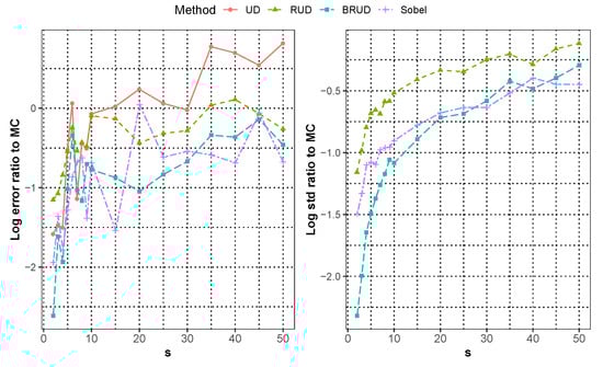
Figure 1. The median approximation error of integration of $f_1\left(x\right)$ over all runs for different dimension.

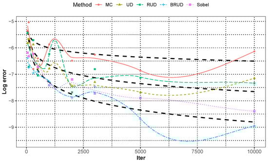
Figure 2. The approximation error of integration 1 for each runs in dimension $s=5$ with locally weighted regression.

Now consider the integral of the functions $f_2\left(x\right)$ and $f_3\left(x\right)$, which are multimodal mixed normal functions. Since they have different means and small variances, they are more concentrated around those means in higher dimensions, which may lead to a poor estimate by using the MC method. Moreover, for $f_2\left(x\right)$, when n is 10,000 and $s\ge 20$, the relative error of the estimated value of the MC or QMC methods is large enough, and the dimension of the integral that can be effectively estimated will decrease. Therefore, we only present the approximation errors of the integral that yield meaningful estimates.

Figure 3 and Figure 4 show the median approximation errors of integration of $f_2\left(\mathit{x}\right)$ and $f_3\left(\mathit{x}\right)$ for all runs in each dimension, and Figure 5 and Figure 6 show the approximation error of integration of $f_2\left(\mathit{x}\right)$ and $f_3\left(\mathit{x}\right)$ when the dimension $s=5$ for each run, respectively. In these two cases, all methods are worse than the previous case of that of $f_1\left(x\right)$. In general, BRUD method is still the best method among these methods. For $f_2\left(\mathit{x}\right)$, only when the dimension is greater than or equal to 15, it is inferior to the MC method. For $f_3\left(\mathit{x}\right)$, all methods are inferior to the MC method in about 6 dimensions. In addition, the convergence rates of the Sobol and BRUD methods are also worse than the previous case, and most of the convergence rates are between $n^{-1/2}$ and $n^{-1}$ for $f_3\left(\mathit{x}\right)$. In Figure 6, the MC method shows significantly better result at the number of iterations more than 5000 in comparison with all other methods. This anomaly is due to the non-smoothness of the function. Moreover, the standard deviation of the MC method is much larger compared to the error at this time, which can produce better results due to randomness. In this case, the BRUD method still has a smaller standard deviation and more stable results.

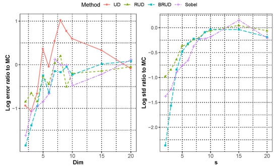
Figure 3. The median approximation error of integration 2 over all runs for dimension $s\le$ 20.

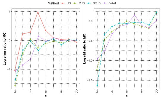
Figure 4. The median approximation error of integration 3 over all runs for dimension $s\le$ 10.

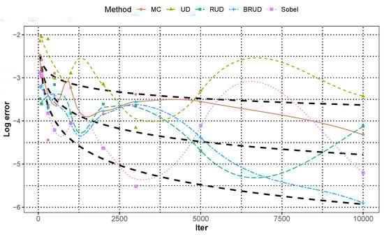
Figure 5. The approximation error of integration 2 for each runs in dimension $s=5$ with Locally Weighted Regression.

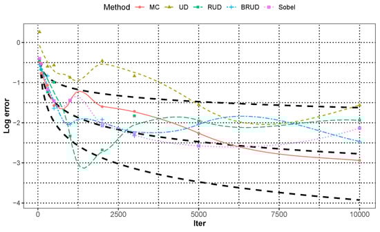
Figure 6. The approximation error of integration 3 for each runs in dimension $s=5$ with Locally Weighted Regression.

In addition, we consider a complex test function from [36] for comparison,

$$\begin{array}{cc}\hfill g\left(x\right)=\prod _{k=1}^s\left(1+\frac{{\omega }^k}{21}(-10+42x_k^2-42x_k^5+21x_k^6)\right)& \hfill \end{array}$$

(6)

This function integrates to 1 over ${[0,1]}^s$. The parameter $\omega$ acts like a product weighht ${\omega }^k$, and we choose $\omega =0.9$.

In this case, the function $g\left(x\right)$ is a product of $1+{\omega }^k(B_6\left(x_k\right)+E_5\left(x_k\right))$, where $B_6$ is the degree 6 Bernoulli polynomial and $E_5$ is the degree 5 Euler polynomial. It is a sufficiently smooth function, but differs from the previous functions in that it is non-separable and has a product parameter $\omega$. Figure 7 and Figure 8 show the performance of different methods for the integration of $g\left(x\right)$. The BRUD method and Sobel method still perform well in terms of the estimation error, standard deviation, and convergence rate of order, and the BRUD method has a significant advantage in low dimensions, but the Sobel method is superior in high dimensions.

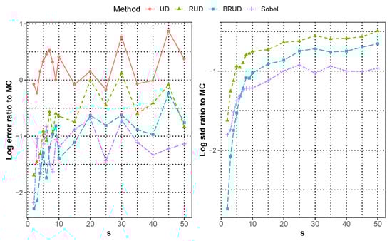
Figure 7. The median approximation error of integration of $g\left(x\right)$ over all runs for different dimension.

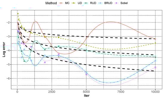
Figure 8. The approximation error of integration of $g\left(x\right)$ for each runs in dimension $s=5$ with Locally Weighted Regression.

From the numerical experimental results, the BRUD method has better results and shows faster convergence rates than other methods for functions with sufficient smoothness or lower dimensionality, where the effect of function smoothness on the convergence rate is a bit more significant. The requirement for smoothness condition in [35] is that the mixed partial derivatives of the integrand of order two or less in each coordinate be square integrable. All QMC methods are less effective compared to MC methods when the dimension of the function becomes higher or when the function is very non-smooth. The BRUD method is much better than other QMC methods in low dimensions, although it is not as good as other QMC methods in some high dimensional cases.

6. Conclusions

In this paper, we theoretically derive the order of convergence rate of the centered $L_2$-discrepancy, wrap-around $L_2$-discrepancy and mixture discrepancy. Using the uniform design obtained from the numerical search by MD, we propose a randomized quasi-Monte Carlo method based on randomization and the Baker’s transformation. Numerical studies show that, the proposed method has a great advantage over the Monte Carlo method and other quasi-Monte Carlo methods in terms of estimation error and standard deviation, especially for the dimension $s\le 10$.

References

- Leobacher, G.; Pillichshammer, F. Introduction to Quasi-Monte Carlo Integration and Applications; Birkhuser: Basel, Switzerland, 2014. [Google Scholar]
- Metropolis, N. The beginning of the monte-carlo method. In Los Alamos Sci. 1987, 125–130. [Google Scholar]
- Richtmyer, R.D. The evaluation of definite integrals and a quasi-monte carlo method based on the properties of algebraic numbers. Differ. Equ. 1951.
- Halton, J.H. On the efficiency of certain quasi-random sequences of points in evaluating multi-dimensional integrals. Numer. Math. 1960, 2, 84–90. [Google Scholar] [CrossRef]
- Sobol, I.M. The distribution of points in a cube and the approximate evaluation of integrals. USSR Comput. Math. Math. Phys. 1969, 7, 784–802. [Google Scholar] [CrossRef]
- Faure, H. Discrépance des suites associées à un systéme de numération. Acta Arith. 1982, 41, 337–351. [Google Scholar] [CrossRef]
- Collings, B.J.; Niederreiter, H. Random number generation and quasi-monte carlo methods. J. Am. Stat. Assoc. 1993, 699. [Google Scholar] [CrossRef]
- Shu, T. Uniform Random Numbers: Theory and Practice; Springer: Berlin/Heidelberg, Germany, 1995. [Google Scholar]
- Joe, S.; Kuo, F.Y. Constructing sobol’ sequences with better two-dimensional projections. SIAM J. Sci. Comput. 2008, 30, 2635–2654. [Google Scholar] [CrossRef]
- Korobov, N.M. The approximate computation of multiple integrals. Dokl. Akad. Nauk. SSSR 1959, 124, 1207–1210. [Google Scholar]
- Korobov, N.M. Properties and calculation of optimal coefficients. Dokl. Akad. Nauk. 1960, 132, 1009–1012. [Google Scholar]
- Hlawka, E. Zur angenäherten berechnung mehrfacher integrale. Monatshefte Math. 1962, 66, 140–151. [Google Scholar] [CrossRef]
- Fang, K.T. The uniform design: Application of number-theoretic methods in experimental design. Acta Math. Appl. Sin. 1980, 3, 9. [Google Scholar]
- Wang, Y.; Fang, K.T. A note on uniform distribution and experimental design. Kexue Tongbao 1981, 26, 485–489. [Google Scholar]
- Patterson, R. Randomization of number theoretic methods for multiple integration. Siam J. Numer. Anal. 1976, 13, 904–914. [Google Scholar]
- Tuffin, B. On the use of low discrepancy sequences in monte carlo methods. Monte Carlo Methods Appl. 1998, 4, 87–90. [Google Scholar] [CrossRef]
- Morohosi, H.; Fushimi, M. A Practical Approach to the Error Estimation of Quasi-Monte Carlo Integrations. In Monte-Carlo and Quasi-Monte Carlo Methods; Springer: Berlin/Heidelberg, Germany, 1998. [Google Scholar]
- Owen, A.B. Scrambling sobol’ and niederreiter-xing points. J. Complex. 1998, 14, 466–489. [Google Scholar] [CrossRef]
- Owen, A.B.; Niederreiter, H.; Shiue, J.S. Randomly permuted (t,m,s)-nets and (t,s)-sequences. In Monte Carlo and Quasi-Monte Carlo Methods in Scientific Computing; Springer: New York, NY, USA, 1995. [Google Scholar]
- Matoušek, J. On the l2-discrepancy for anchored boxes. J. Complex. 1998, 14, 527–556. [Google Scholar]
- Wang, X.; Hickernell, F.J. Randomized halton sequences. Math. Comput. Model. 2000, 32, 887–899. [Google Scholar] [CrossRef]
- Dick, J.; Pillichshammer, F. Digital Nets and Sequences: Discrepancy Theory and Quasi-Monte Carlo Integration; Cambridge University Press: Cambridge, UK, 2010. [Google Scholar]
- Hickernell, F.J. A generalized discrepancy and quadrature error bound. Math. Comput. 1998, 67, 299–322. [Google Scholar] [CrossRef]
- Hickernell, F.J. Lattice rules: How well do they measure up? In Random and Quasi-Random Point Sets; Hellekalek, P., Larcher, G., Eds.; Springer: Berlin/Heidelberg, Germany, 1998; pp. 106–166. [Google Scholar]
- Zhou, Y.D.; Fang, K.T.; Ning, J.H. Mixture discrepancy for quasi-random point sets. J. Complex. 2013, 29, 283–301. [Google Scholar] [CrossRef]
- Fang, K.T.; Liu, M.Q.; Qin, H.; Zhou, Y. Theory and Application of Uniform Experimental Designs; Springer and Science Press: Singapore, 2018. [Google Scholar]
- Glasserman, P. Monte Carlo Methods in Financial Engineering; Springer: New York, NY, USA, 2003. [Google Scholar]
- Hammersley, J.M.; Handscomb, D.C. Monte Carlo Methods; Springer: Berlin/Heidelberg, Germany, 2013. [Google Scholar]
- Bakhvalov, N.S. On the approximate calculation of multiple integrals. J. Complex. 2015, 31, 502–516. [Google Scholar] [CrossRef]
- Koksma, J.F. A general theorem from the theory of uniform distribution modulo 1. Banks Filip Saidak Mayumi 1942, 7–11. [Google Scholar]
- Hlawka, E. Funktionen von beschränkter variatiou in der theorie der gleichverteilung. Ann. Mat. Pura Appl. 1961, 54, 325–333. [Google Scholar] [CrossRef]
- Hickernell, F.J.; Liu, M. Uniform designs limit aliasing. Biometrika 2002, 89, 893–904. [Google Scholar] [CrossRef]
- Hua, L.K.; Wang, Y. Applications of Number Theory to Numerical Analysis; Springer: Berlin, Germany; Science Press: Beijing, China, 1981. [Google Scholar]
- L’Ecuyer, P.; Lemieux, C. Recent advances in randomized quasi-monte carlo methods. Modeling Uncertainty; Springer: New York, NY, USA, 2002; pp. 419–474. [Google Scholar]
- Hickernell, F.J. Obtaining O(n−2+ϵ) convergence for lattice quadrature rules. In Monte Carlo and Quasi-Monte Carlo Methods; Springer: Berlin/Heidelberg, Germany, 2000; pp. 274–289. [Google Scholar]
- Dick, J.; Nuyens, D.; Pillichshammer, F. Lattice rules for nonperiodic smooth integrands. Numer. Math. 2014, 126, 259–291. [Google Scholar] [CrossRef]
- Hua, L.K. Introduction to Number Theory; Science Press: Beijing, China, 1956. [Google Scholar]
Publisher’s Note: MDPI stays neutral with regard to jurisdictional claims in published maps and institutional affiliations. |
© 2022 by the authors. Licensee MDPI, Basel, Switzerland. This article is an open access article distributed under the terms and conditions of the Creative Commons Attribution (CC BY) license (https://creativecommons.org/licenses/by/4.0/).