An Approximation Method to Compute Highly Oscillatory Singular Fredholm Integro-Differential Equations

Abstract

This paper appertains the presentation of a Clenshaw–Curtis rule to evaluate highly oscillatory Fredholm integro-differential equations (FIDEs) with Cauchy and weak singularities. To calculate the singular integral, the unknown function approximated by an interpolation polynomial is rewritten as a Taylor series expansion. A system of linear equations of FIDEs obtained by using equally spaced points as collocation points is solved to obtain the unknown function. The proposed method attains higher accuracy rates, which are proven by error analysis and some numerical examples as well.

1. Introduction

Integro-differential equations (IDEs) are studied in physics, biology, and engineering applications, as well as in advanced integral equations literature. Applications of the IDEs in electromagnetic theory, dispersive waves, and ocean circulations are enormous [1,2,3,4,5,6]. The addressed paper considers the highly oscillatory singular FIDEs of the following kind:

$$\begin{array}{cc}{\displaystyle \sum _{\mu =0}^{\nu }}{P}_{\mu }\left(x\right)y^{\left(\mu \right)}\left(x\right)& =f\left(x\right)+Q\left(x\right){\int }_{-1}^{1}k(x,t)y\left(t\right)dt,\end{array}$$

(1)

along with the initial condition:

$$y^{\left(\mu \right)}(-1)={\alpha }_{\mu },0\le \mu \le \nu -1.$$

(2)

The given highly oscillatory kernel function $k(x,t)$ possesses weak and Cauchy singularities, i.e., $k(x,t)=\frac{w\left(t\right)e^{ikt}}{t-x},w\left(t\right)={(1+t)}^{\alpha }{(1-t)}^{\beta }$. $P\left(x\right),f\left(x\right),Q\left(x\right)$ are smooth functions on $[-1,1]$, whereas $y\left(x\right)$ is the unknown function that needs to be determined. The FIDEs having weak or strong singularities are considered in [7]. To gain analytical approximation, the author used the power series expansion technique. However, for the convergence of the method, the author applied a ratio test and proved that the proposed method gives exact solutions if the solutions of the equations are finite-degree polynomials. Otherwise, by increasing the number of polynomials, better accuracies are obtained.

For a FIDE of the kind

$$\begin{array}{l}{u}^n\left(t\right)={\displaystyle \sum _{i=0}^{n_0}}{a}_i\left(t\right)u^{\left(i\right)}\left(t\right)+{\displaystyle \sum _{i=0}^{n_0}}{\int }_0^b{k}_i(t,s)u^{\left(i\right)}ds+f\left(t\right),0\le t\le b,\\ \mathrm{with}{\displaystyle \sum _{i=0}^{n-1}}[{\alpha }_{ij}{u}^{\left(i\right)}\left(0\right)+{\beta }_{ij}{u}^{\left(i\right)}\left(b\right)]=0,j=1,2,\cdots ,n,\end{array}$$

(3)

a reproducing kernel method is introduced in [8], where the kernel function in the equation is a weakly singular kernel. The method converts the weakly singular kernel into a logarithmic kernel to a Kalman kernel. Furthermore, a smooth transformation helps to remove the weak singularity of the Kalman kernel. The authors claimed that the reproducing kernel method is not restricted by the order of the equation.

A quadrature formula is applied to discretize the FIDEs. Based on the behavior of the exact solution, the special graded grid points are used for piecewise polynomial collocation method [9]. Smooth parts of the integrands are approximated by the piecewise polynomial interpolation, whereas the singular parts are integrated exactly. By the same authors in [10], two approaches, an integral equation reformation and discrete Galerkin method, are used to find the approximations for the solutions and derivatives of the nth order weakly singular FIDEs. The approximations to the solutions are piecewise polynomial functions. In another research work, the Taylor series expansion along with the Galerkin method is considered for FIDEs with Cauchy singularity. The Legendre polynomials are used as basis to approximate the solution of the FIDEs [11]. The traditional piecewise homotopy perturbation method is extended for FIDEs with weak singular kernels. The accuracy and calculation speed with the Gauss quadrature rule and piecewise low-order interpolation is significantly improved in [12].

For an FIDE

$$\begin{array}{c}{u}^{\prime }\left(t\right)=a\left(t\right)u\left(t\right)+{\int }_0^{b}k(t,s)u\left(s\right)ds+f\left(t\right),0\le t\le b,\\ \mathrm{with} \alpha u\left(0\right)+\beta u\left(b\right)=\gamma ,\alpha ,\beta ,b,\gamma \in (-\infty ,\infty )\mathrm{and}\alpha +\beta \ne 0,\end{array}$$

(4)

with weak singular or other non-smooth kernels, the regularity properties of the solutions are briefly studied by the author in [13]. These obtained results are further used in the analysis to solve such problems by piecewise polynomial collocation method. As compared to highly oscillatory Volterra integral equations, Fredholm integral equations with high oscillations have received less attention by researchers. Nevertheless, there is still a gap to be filled to propose the approximate methods to obtain the numerical solutions of highly oscillatory FIDEs along with the singular kernel functions. The purpose of this paper is to represent an efficient algorithm for such highly oscillatory singular FIDEs and try to fill this gap. The main novelty is the simplicity and accuracy of the proposed method. This research work aims at introducing an approximation method for a highly oscillatory Fredholm integro-differential equation. The general form of the integral term in Equation (1) with highly oscillatory function, weak singularities and Cauchy singularity in $[-1,1]$ is defined as ${⨍}_{-1}^1\frac{w\left(t\right)y\left(t\right)e^{ikt}}{t-x}dt,w\left(t\right)={(1+t)}^{\alpha }{(1-t)}^{\beta }$, $-1<\alpha ,\beta <1$, $x\in (-1,1)$.

Along with weak and Cauchy singularities, the highly oscillatory FIDE (1) is impossible to solve by the classical methods discussed above. To overcome such adversity, an approximated method following the steps of the Clenshaw–Curtis rule is presented, which interpolates the unknown function with an interpolation polynomial $H_N\left(x\right)$ of degree N. In the integral term, the interpolation polynomial extended to a sum of Chebyshev series of the first kind is rewritten in the form of truncated Taylor series expansion for $x\in (-1,1)$. The pivotal point of this method is that efficient results with higher accuracy rates can be achieved for smaller values of N and m, where m defines the degree of the Taylor series expansion of the Chebyshev polynomial. With the evaluation of the highly oscillatory singular integral, a system of linear equations is constructed for Equation (1) by using the equally spaced points as the collocation points. This system is eventually solved to obtain the unknown coefficients for the unknown function $y\left(x\right)$.

The rest of this paper is organized as follows: Section 2 illustrates the methodology of a newly proposed method briefly, and obtains a system of linear equations. Section 3 gives an idea of error estimation. The efficiency and accuracy of the method is demonstrated in Section 4 by some numerical examples.

2. Methodology

A function $y\left(x\right)$ can be approximated by its interpolation polynomial $H_N\left(x\right)$ of degree N at Chebyshev points of the second kind, $x_j=\cos \frac{j\pi }{N},j=0,1,\cdots N$. We rewrite the interpolation polynomial in terms of the Chebyshev series as [14]:

$$\begin{array}{cc}y\left(x\right)\approx H_N\left(x\right)=& {\displaystyle \sum _{n=0}^N}{}^{″}{a}_n{T}_n\left(x\right),\end{array}$$

(5)

where $T_n\left(x\right)$ is the Chebyshev polynomial of the first kind of degree n, double prime denotes a sum whose first and last term are halved and $a_n$ are the coefficients which can be efficiently computed by FFT [15,16], defined as

$$a_n=\frac{2}{N}{\displaystyle \sum _{j=0}^N}{}^{″}y\left(x_j\right)T_n\left(x_j\right).$$

Equation (5) can further be written in the matrix form as follows:

$$\begin{array}{c}y\left(x\right)=\mathbf{T}\left(x\right)\mathbf{A},\\ \mathbf{T}=[T_0\left(x\right),T_1\left(x\right),\cdots ,T_N\left(x\right)],\mathbf{A}={[a_0,a_1,\cdots ,a_N]}^T.\end{array}$$

(6)

Furthermore, the derivative of a function $y^{\left(\mu \right)}\left(x\right), \mu =0,1,\cdots ,$ in terms of Chebyshev series and matrix form is defined as [17]

$$\begin{array}{c}{y}^{\left(\mu \right)}\left(x\right)=\mathbf{T}\left(x\right){\mathbf{A}}^{\left(\mu \right)},\\ y^{\left(\mu \right)}\left(x\right)=2^{\mu }\mathbf{T}\left(x\right){\mathbf{M}}^{\left(\mu \right)}\mathbf{A},\end{array}$$

(7)

where the matrix ${\mathbf{M}}_{(N+1)\times (N+1)}$ for odd and even values of N is defined, respectively, as:

$$\mathbf{M}={\left[\begin{array}{cccccccc}0& 1/2& 0& 3/2& 0& 5/2& \cdots & N/2\\ 0& 0& 2& 0& 4& 0& \cdots & 0\\ 0& 0& 0& 3& 0& 5& \cdots & N\\ ⋮& ⋮& ⋮& ⋮& ⋮& \cdots & ⋮& \\ 0& 0& 0& 0& 0& 0& \cdots & N\\ 0& 0& 0& 0& 0& 0& \cdots & 0\end{array}\right]}_{(N+1)\times (N+1)},$$

$$\mathbf{M}={\left[\begin{array}{cccccccc}0& 1/2& 0& 3/2& 0& 5/2& \cdots & 0\\ 0& 0& 2& 0& 4& 0& \cdots & N\\ 0& 0& 0& 3& 0& 5& \cdots & 0\\ ⋮& ⋮& ⋮& ⋮& ⋮& ⋮& \cdots & ⋮\\ 0& 0& 0& 0& 0& 0& \cdots & N\\ 0& 0& 0& 0& 0& 0& \cdots & 0\end{array}\right]}_{(N+1)\times (N+1)}.$$

By considering the Equation (5) for integral ${⨍}_{-1}^1\frac{w\left(t\right)y\left(t\right)e^{ikt}}{t-x}dt$ in (1), it transforms into the following:

$${⨍}_{-1}^1\frac{{\sum }_{n=0}^N{}^{″}w\left(t\right)a_n{T}_n\left(t\right)e^{ikt}}{t-x}dt={\displaystyle \sum _{n=0}^N}{a}_n{R}_n(x,k),$$

(8)

where $R_n(x,k)$ are called the modified moments and defined as:

$$R_n(x,k)=\left\{\begin{array}{ll}{B}_n(x,k)={⨍}_{-1}^1\frac{T_n\left(t\right)e^{ikt}}{t-x}dt,& \mathrm{for}w\left(t\right)=1,\\ B_n(x,k,\alpha ,\beta )={⨍}_{-1}^1\frac{w\left(t\right)T_n\left(t\right)e^{ikt}}{t-x}dt,& \mathrm{for}w\left(t\right)\ne 1.\end{array}\right.$$

The following subsection appertains the Clenshaw–Curtis method with truncated Taylor series to evaluate the moments $R_n(x,k)$ accurately.

2.1. Computation of the $B_n(x,k)$ Moments

For moments $B_n(x,k)$, we transform these moments into a singular and non-singular integrals by applying some basic steps as follows:

$${⨍}_{-1}^1\frac{T_n\left(t\right)e^{ikt}}{t-x}dt={\int }_{-1}^1\frac{T_n\left(t\right)-T_n\left(x\right)}{t-x}{e}^{ikt}dt+T_n\left(x\right){⨍}_{-1}^1\frac{e^{ikt}}{t-x}dt.$$

(9)

For the Cauchy singular integral ${⨍}_{-1}^1\frac{e^{ikt}}{t-x}dt$, an explicit calculation has been performed in [16] as

$${⨍}_{-1}^1\frac{e^{ikt}}{t-x}dt=e^{ikx}[sgn\left(k\right)\pi i+E_1\left(ik(1+x)\right)-E_1\left(ik(x-1)\right)],$$

(10)

where $E_1\left(z\right)={\int }_z^{\infty }\frac{e^{-t}}{t}dt$ is the exponential integral, and $sgn\left(x\right)$ is the sign function. On the other hand, by applying the truncated Taylor series expansion for $T_n\left(t\right)$ in non-singular integral, we obtain

$$\begin{array}{l}{\int }_{-1}^1\frac{T_n\left(t\right)-T_n\left(x\right)}{t-x}{e}^{ikt}dt={\int }_{-1}^1\frac{[(t-x)T_n^{\prime }\left(x\right)+\frac{{(t-x)}^2}{2!}{T}_n^{″}\left(x\right)+\cdots +\frac{{(t-x)}^m}{m!}{T}_n^m\left(x\right)]}{t-x}{e}^{ikt}dt\\ =T_n^{{}^{\prime }}\left(x\right){\int }_{-1}^1{e}^{ikt}dt+\frac{T_n^{{}^{″}}\left(x\right)}{2!}{\int }_{-1}^1(t-x)e^{ikt}dt+\cdots +\frac{T_n^m\left(x\right)}{m!}{\int }_{-1}^1{(t-x)}^{m-1}{e}^{ikt}dt\\ =[T_n^{{}^{\prime }}\left(x\right),\frac{T_n^{{}^{″}}\left(x\right)}{2!},\cdots ,\frac{T_n^m\left(x\right)}{m!}]{[A^0,A^1,\cdots ,A^{m-1}]}^T,\end{array}$$

(11)

where

$$A^0={\int }_{-1}^1{e}^{ikt}dt,A^1={\int }_{-1}^1(t-x)e^{ikt}dt,A^{m-1}={\int }_{-1}^1{(t-x)}^{m-1}{e}^{ikt}dt.$$

To calculate the moments $A^m$, a simple recurrence relation is illustrated by integrating by parts

$$\begin{array}{l}{A}^m={\int }_{-1}^1{(t-x)}^m{e}^{ikt}dt\\ A^m={(1-x)}^m\frac{e^{ikt}}{ik}-{(-1-x)}^m\frac{e^{-ikt}}{ik}+\frac{m}{ik}{A}^{m-1},m\ge 1,\end{array}$$

(12)

with the initial value $A^0=\frac{e^{ikt}-e^{-ikt}}{ik}$, where m denotes the derivatives of the relative terms.

2.2. Computation of the $B_n(x,k,\alpha ,\beta )$ Moments

For the moments $B_n(x,k,\alpha ,\beta )={⨍}_{-1}^1\frac{w\left(t\right)T_n\left(t\right)e^{ikt}}{t-x}dt$, by following the initial necessary steps as above, we obtain

$${⨍}_{-1}^1\frac{w\left(t\right)T_n\left(t\right)e^{ikt}}{t-x}dt={\int }_{-1}^1\frac{w\left(t\right)(T_n\left(t\right)-T_n\left(x\right))}{t-x}{e}^{ikt}dt+T_n\left(x\right){⨍}_{-1}^1\frac{w\left(t\right)e^{ikt}}{t-x}dt.$$

(13)

In addition, by applying the truncated Taylor series expansion for the left integral, it becomes

$$\begin{array}{cc}& {\int }_{-1}^1\frac{w\left(t\right)(T_n\left(t\right)-T_n\left(x\right))}{t-x}{e}^{ikt}dt=[T_n^{{}^{\prime }}\left(x\right),\frac{T_n^{{}^{″}}\left(x\right)}{2!},\cdots ,\frac{T_n^m\left(x\right)}{m!}]{[{\tilde{A}}^0,{\tilde{A}}^1,\cdots ,{\tilde{A}}^{m-1}]}^T,\end{array}$$

(14)

where

$${\tilde{A}}^m={\int }_{-1}^{1}w\left(t\right){(t-x)}^m{e}^{ikt}dt,m\ge 0.$$

${\tilde{A}}^m$ clearly possesses some weak singularities as well as high oscillation and cannot be calculated easily without any numerical method. The following theorem presents the steepest descent method to evaluate this integral significantly accurately.

Theorem 1.

Suppose that a function $g\left(t\right)$ is analytic in the half-strip of the complex plane $-1\le \Re \left(x\right)\le 1$ and $\Im \left(x\right)\ge 0$, and satisfies that

$${\int }_{-1}^1\left|g(t+iR)\right|dt\le M{R}^{\alpha +\beta +m}{e}^{k_{0}R},0<k_0<k,$$

(15)

for M and $k_0$ constants, the integral $I\left[g\right]={\int }_{-1}^{1}g\left(t\right)w\left(t\right){(t-x)}^m{e}^{ikt}dt$ can be evaluated as

$$\begin{array}{ll}I\left[g\right]& =\frac{i^{1+\alpha }{e}^{-ik}}{k^{1+\alpha }}{\int }_0^{\infty }g\left(-1+\frac{it}{k}\right){\left(2-\frac{it}{k}\right)}^{\beta }{\left(-1+\frac{it}{k}-x\right)}^m{t}^{\alpha }{e}^{-t}dt\\ & +\frac{{(-1)}^{\beta }{\left(i\right)}^{\beta +1}{e}^{ik}}{k^{1+\beta }}{\int }_0^{\infty }g\left(1+\frac{it}{k}\right){\left(2+\frac{it}{k}\right)}^{\alpha }{\left(1+\frac{it}{k}-x\right)}^m{t}^{\beta }{e}^{-t}dt.\end{array}$$

(16)

Proof. 

The integrand $g\left(t\right)w\left(t\right){(t-x)}^m{e}^{ikt}$ is analytic in the half-strip of the complex plane: $-1\le \Re \left(x\right)\le 1$ and $\Im \left(x\right)\ge 0$; then, based on the Cauchy’s theorem, we obtain

$${\int }_{{\Gamma }_1+{\Gamma }_2+{\Gamma }_3+{\Gamma }_4+{\Gamma }_5+{\Gamma }_6+{\Gamma }_m}g\left(t\right)w\left(t\right){(t-x)}^m{e}^{ikt}dt=0,$$

(17)

where paths of the integration are taken in counterclockwise direction and shown in the Figure 1.

Figure 1. The integration path for integral $I\left[g\right]$.

Since ${\Gamma }_1=1+ip,p\in [r,R]$, where R is a large number, then

$$\begin{array}{ll}{\int }_{{\Gamma }_1}& ={\int }_r^{R}g(1+ip){(2+ip)}^{\alpha }{(-ip)}^{\beta }{(1+ip-x)}^m{e}^{ik(1+ip)}idp\\ & =\frac{{(-1)}^{\beta }{i}^{1+\beta }{e}^{ik}}{k^{1+\beta }}{\int }_{kr}^{kR}g\left(1+\frac{it}{k}\right){\left(2+\frac{it}{k}\right)}^{\alpha }{(1+\frac{it}{k}-x)}^m{t}^{\beta }{e}^{-t}dt.\end{array}$$

Similarly,

$${\int }_{{\Gamma }_3}=-\frac{i^{1+\alpha }{e}^{-ik}}{k^{1+\alpha }}{\int }_{kr}^{kR}g\left(-1+\frac{it}{k}\right){\left(2-\frac{it}{k}\right)}^{\beta }{(-1+\frac{it}{k}-x)}^m{t}^{\alpha }{e}^{-t}dt.$$

In addition,

$$\begin{array}{ll}\left|{\int }_{{\Gamma }_2}\right|& =\left|{\int }_{-1}^{1}g(t+iR)e^{ik(t+iR)}{(t+iR+1)}^{\alpha }{(1-t-iR)}^{\beta }{(t+iR-x)}^{m}dt\right|\\ & \le e^{-kR}{\int }_{-1}^1\left|g(t+iR){(t+iR+1)}^{\alpha }{(1-t-iR)}^{\beta }{(t+iR-x)}^m\right|dt\to 0,\mathrm{as}R\to \infty .\end{array}$$

For ${\Gamma }_0$, by taking $t+1=r{e}^{i\theta }$ and $0\le \theta \le \frac{\pi }{2}$,

$$\begin{array}{c}{\int }_{{\Gamma }_0}=-ir{e}^{-ik}{\int }_0^{\frac{\pi }{2}}g(-1+r{e}^{i\theta })e^{ikr{e}^{i\theta }}{e}^{i\theta }{\left(r{e}^{i\theta }\right)}^{\alpha }{(2-r{e}^{i\theta })}^{\beta }{(-1+r{e}^{i\theta }-x)}^{m}d\theta \end{array}$$

(18)

then

$$\begin{array}{l}|{\int }_0^{\frac{\pi }{2}}g(-1+r{e}^{i\theta }){(2-r{e}^{i\theta })}^{\beta }{(-1+r{e}^{i\theta }-x)}^m{e}^{ikr{e}^{i\theta }}{e}^{i(1+\alpha )\theta }d\theta -{\int }_0^{\frac{\pi }{2}}g(-1)2^{\beta }{(-1-x)}^m{e}^{i(1+\alpha )\theta }d\theta |\\ =|{\int }_0^{\frac{\pi }{2}}g(-1+r{e}^{i\theta }){(2-r{e}^{i\theta })}^{\beta }{(-1+r{e}^{i\theta }-x)}^m{e}^{ikr{e}^{i\theta }}{e}^{i(1+\alpha )\theta }d\theta -{\int }_0^{\frac{\pi }{2}}g(-1)2^{\beta }{(-1-x)}^m{e}^{ikr{e}^{i\theta }}{e}^{i(1+\alpha )\theta }d\theta \\ +{\int }_0^{\frac{\pi }{2}}g(-1)2^{\beta }{(-1-x)}^m{e}^{ikr{e}^{i\theta }}{e}^{i(1+\alpha )\theta }d\theta -{\int }_0^{\frac{\pi }{2}}g(-1)2^{\beta }{(-1-x)}^m{e}^{i(1+\alpha )\theta }d\theta |\\ \le {\int }_0^{\frac{\pi }{2}}{e}^{-krsin\left(\theta \right)}|g(-1+r{e}^{i\theta }){(2-r{e}^{i\theta })}^{\beta }{(-1+r{e}^{i\theta }-x)}^m-g(-1)2^{\beta }{(-1-x)}^m|d\theta \\ +\left|g(-1)\right|2^{\beta }{(-1-x)}^m{\int }_0^{\frac{\pi }{2}}|e^{ikr{e}^{i\theta }}-1|d\theta \\ \le {\int }_0^{\frac{\pi }{2}}|g(-1+r{e}^{i\theta }){(2-r{e}^{i\theta })}^{\beta }{(-1+r{e}^{i\theta }-x)}^m-g(-1)2^{\beta }{(-1-x)}^m|d\theta \\ +\left|g(-1)\right|2^{\beta }{(-1-x)}^m{\int }_0^{\frac{\pi }{2}}|e^{ikr{e}^{i\theta }}-1|d\theta .\end{array}$$

It follows

$$\begin{array}{c}|{\int }_0^{\frac{\pi }{2}}g(-1+r{e}^{i\theta }){(2-r{e}^{i\theta })}^{\beta }{(-1+r{e}^{i\theta }-x)}^m{e}^{ikr{e}^{i\theta }}{e}^{i(1+\alpha )\theta }d\theta -{\int }_0^{\frac{\pi }{2}}g(-1)2^{\beta }{(-1-x)}^m{e}^{i(1+\alpha )\theta }d\theta |\to 0,r\to 0.\end{array}$$

For $r\to 0$, there exist

$$\begin{array}{ll}{\int }_0^{\frac{\pi }{2}}g(-1+r{e}^{i\theta }){(2-r{e}^{i\theta })}^{\beta }{(-1+r{e}^{i\theta }-x)}^m{e}^{ikr{e}^{i\theta }}{e}^{i(1+\alpha )\theta }d\theta & ={\int }_0^{\frac{\pi }{2}}g(-1)2^{\beta }{(-1-x)}^m{e}^{i(1+\alpha )\theta }d\theta \\ & =\frac{g(-1)2^{\beta }{(-1-x)}^m}{i(1+\alpha )}[e^{i(1+\alpha )\frac{\pi }{2}}-1].\end{array}$$

(19)

By Equations (19) and (18), we yield

$${\int }_{{\Gamma }_0}g\left(t\right)w\left(t\right){(t-x)}^m{e}^{ikt}dt\to 0,r\to 0.$$

Similarly, for all integration paths ${\Gamma }_m\to 0,r\to 0.$

For $r\to 0,R\to \infty$, Equation (17) implies

$$\underset{r\to 0,R\to \infty }{lim}{\int }_{{\Gamma }_4+{\Gamma }_5+{\Gamma }_6}g\left(t\right)w\left(t\right){(t-x)}^m{e}^{ikt}dt=-\underset{r\to 0,R\to \infty }{lim}{\int }_{{\Gamma }_1+{\Gamma }_2+{\Gamma }_3+{\Gamma }_m}g\left(t\right)w\left(t\right){(t-x)}^m{e}^{ikt}dt=0.$$

(20)

  □

For the calculation of integrals involving weight functions $t^{\alpha }{e}^{-t}$ and $t^{\beta }{e}^{-t}$, the generalized Gauss–Laguerre quadrature rule can be used to approximate these integrals. For this purpose, let $x_j$ and $w_j$ be the zeros and weight functions of generalized Gauss–Laguerre quadrature rule, respectively, then these integrals are written as

$$\begin{array}{ll}{\widehat{Q}}_l\left[g\right]& =\frac{i^{1+\alpha }{e}^{-ik}}{k^{1+\alpha }}{\displaystyle \sum _{j=1}^l}{w}_{j}g\left(-1+\frac{i{t}_j}{k}\right){\left(2-\frac{i{t}_j}{k}\right)}^{\beta }{\left(-1+\frac{i{t}_j}{k}-x\right)}^m\\ & +\frac{{(-1)}^{\beta }{\left(i\right)}^{\beta +1}{e}^{ik}}{k^{1+\beta }}{\displaystyle \sum _{j=1}^l}{w}_{j}g\left(1+\frac{i{t}_j}{k}\right){\left(2+\frac{i{t}_j}{k}\right)}^{\alpha }{\left(1+\frac{i{t}_j}{k}-x\right)}^m.\end{array}$$

(21)

The above theorem is proved for a highly oscillatory weakly singular integral which has an analytic function; however, this can be extended to the integral ${\tilde{A}}_m$ of our choice.

The integral ${⨍}_{-1}^1\frac{w\left(t\right)e^{ikt}}{t-x}dt$ in Equation (13) is also explicitly calculated by steepest descent method in [18,19].

With the successful evaluation of the moments $R_n(x,k)$, the Equation (1) is transformed after some necessary substitutions as

$${\displaystyle \sum _{\mu =0}^{\nu }}{2}^{\mu }{P}_{\mu }\left(x\right)\mathbf{T}\left(x\right){\mathbf{M}}^{\left(\mu \right)}\mathbf{A}=f\left(x\right)+Q\left(x\right)\mathbf{A}{R}_n(x,k).$$

(22)

Furthermore, to obtain the unknown coefficients $\mathbf{A}$ in Equation (22), we can apply collocation method for equally spaced points $x_i$ as

$${\displaystyle \sum _{\mu =0}^{\nu }}{2}^{\mu }{\mathbf{P}}_{\mu }\mathbf{T}\left(x_i\right){\mathbf{M}}^{\left(\mu \right)}\mathbf{A}=\mathbf{F}+\mathbf{Q}\mathbf{A}\mathbf{R}(x_i,k),$$

(23)

where

$${\mathbf{P}}_{\mu }=\left[\begin{array}{cccc}{P}_{\mu }\left(x_0\right)& 0& \cdots & 0\\ 0& P_{\mu }\left(x_1\right)& \cdots & 0\\ ⋮& ⋮& \ddots & ⋮\\ 0& 0& \cdots & P_{\mu }\left(x_N\right)\end{array}\right],\mathbf{Q}=\left[\begin{array}{cccc}Q\left(x_0\right)& 0& \cdots & 0\\ 0& Q\left(x_1\right)& \cdots & 0\\ ⋮& ⋮& \ddots & ⋮\\ 0& 0& \cdots & Q\left(x_N\right)\end{array}\right],$$

$$\mathbf{R}(x_i,k)=\left[\begin{array}{cccc}{R}_0(x_0,k)& R_1(x_0,k)& \cdots & R_n(x_0,k)\\ R_0(x_1,k)& R_1(x_1,k)& \cdots & R_n(x_1,k)\\ ⋮& ⋮& \ddots & ⋮\\ R_0(x_N,k)& R_1(x_N,k)& \cdots & R_n(x_N,k)\end{array}\right],\mathbf{T}=\left[\begin{array}{c}\mathbf{T}\left(x_0\right)\\ \mathbf{T}\left(x_1\right)\\ ⋮\\ \mathbf{T}\left(x_N\right)\end{array}\right],\mathbf{F}=\left[\begin{array}{c}f\left(x_0\right)\\ f\left(x_1\right)\\ ⋮\\ f\left(x_N\right)\end{array}\right].$$

For unknown coefficient vector $\mathbf{A}$, the Equation (23) is obtained in matrix form

$$\begin{array}{r}\left({\displaystyle \sum _{\mu =0}^{\nu }}{2}^{\mu }{\mathbf{P}}_{\mu }\mathbf{T}\left(x_i\right){\mathbf{M}}^{\left(\mu \right)}-\mathbf{Q}\mathbf{R}(x_i,k)\right)\mathbf{A}=\mathbf{F}\\ \mathbf{WA}=\mathbf{F},\end{array}$$

(24)

where $\mathbf{W}$ is an $(n+1)\times (n+1)$ matrix and corresponds to a system of linear equations that can be solved to obtain the unknown coefficients $\mathbf{A}$. Similarly for the initial conditions (2), we obtain

$$\begin{array}{cc}{y}^{\left(\mu \right)}(-1)& =2^{\mu }\mathbf{T}(-1){\mathbf{M}}^{\left(\mu \right)}\mathbf{A}={\alpha }_{\mu }.\end{array}$$

(25)

Consequently, by replacing the rows of $\mathbf{W}$ with the rows of Equation (25), the new obtained system of equations $\tilde{\mathbf{W}}\mathbf{A}=\mathbf{F}$ is solved for the unknown coefficients $\mathbf{A}$. Once the unknown coefficients are derived, these can be substituted in the Equation (5) to obtain the unknown function $y\left(x\right)$. It should be noted that the matrix $\mathbf{W}$ of the linear system of equations $\mathbf{WA}=\mathbf{F}$ (24) can be ill-conditioned, which indicates that increasing the parameter N does not guarantee the greater accuracy of the approximated solution. To avoid such adversity, small values of N are taken as the proposed method, giving more accurate results for smaller N. The value of the N in numerical examples is taken as $N\le 15$. The increment in the N values gives no such improvement in the accuracy.

3. Error Analysis

Theorem 2

([15]). A Lipschitz continuous function f on [−1, 1] has a unique representation as a Chebyshev series

$$f\left(x\right)={\displaystyle \sum _{j=0}^{\infty }}{a}_j{T}_j\left(x\right),$$

(26)

which is absolutely and uniformly convergent. The coefficients are given for $j\ge 1$ by the formula

$$a_j=\frac{2}{\pi }{\int }_{-1}^1\frac{f\left(x\right)T_j\left(x\right)}{\sqrt{1-x^2}}dx,$$

(27)

for $j=0$, the factor $\frac{2}{\pi }$ changes to $\frac{1}{\pi }$.

Lemma 1

([15,20]).

• If f is analytic with $\left|f\right(z\left)\right|\le M$ in the region bounded by the ellipse with foci $\pm 1$ and major and minor semiaxis lengths summing to $\rho >1$, then for each $j\ge 0,$

  $$|a_j|\le \frac{2M}{{\rho }^j}.$$

  (28)
• For an integer ${\kappa }_0\ge 0$, let f and its derivatives through $f^{({\kappa }_0-1)}$ be absolutely continuous on $[-1,1]$ and suppose the ${\kappa }_{0}th$ derivative of bounded variation $V_{{\kappa }_0}$. Then for $j\ge {\kappa }_0+1$, the Chebyshev coefficients of f satisfy:

  $$|a_j|\le \frac{2V_{{\kappa }_0}}{\pi j(j-1)\cdots (j-\nu )}.$$

  (29)

Theorem 3.

Suppose that $y\left(t\right)$ is an analytic function and satisfies the conditions of the Theorem 1; then, the error bound for the integral $I\left[y\right]={\int }_{-1}^{1}w\left(t\right)y\left(t\right){(t-x)}^m{e}^{ikt}dt,m\ge 0,$ is denoted as

$$I\left[y\right]-{\widehat{Q}}_l\left[y\right]=E\left[y\right]=O\left(\frac{l!}{2l!}min\left\{\frac{\Gamma (l+\alpha +1)}{k^{2l+\alpha +1}},\frac{\Gamma (l+\beta +1)}{k^{2l+\beta +1}}\right\}\right),k\gg 1.$$

(30)

Proof. 

For integral ${\int }_0^{+\infty }f\left(x\right)x^{\sigma }{e}^{-x}dx,\sigma >-1$, the error formula for the $l$−point general Gauss–Laguerre quadrature rule is defined as [21]

$$\frac{l!\Gamma (l+\sigma +1)}{\left(2l\right)!}{f}^{\left(2l\right)}\left(\zeta \right),0<\zeta <+\infty .$$

(31)

By applying the above formula for the error $E\left[y\right]$, we obtain

$$\begin{array}{ll}E\left[y\right]& \le \frac{l!\Gamma (l+\alpha +1)}{k^{1+\alpha }(2l!)}|\left[f(-1+\frac{it}{k}){(2-\frac{it}{k})}^{\beta }{(-1-x+\frac{it}{k})}^m\right]{|}_{t={\xi }_1}^{2l}\\ & +\frac{l!\Gamma (l+\beta +1)}{k^{1+\beta }(2l!)}|\left[f(1+\frac{it}{k}){(2+\frac{it}{k})}^{\alpha }{(1-x+\frac{it}{k})}^m\right]{|}_{t={\xi }_2}^{2l}\\ & =\frac{l!}{\left(2l\right)!}\left\{\frac{\Gamma (l+\alpha +1)}{k^{2l+\alpha +1}}\right|\left[f(-1+i{\zeta }_1){(2-i{\zeta }_1)}^{\beta }{(-1-x+i{\zeta }_1)}^m\right]{|}_{{\zeta }_1=\frac{{\xi }_1}{k}}^{2l}\\ & +\frac{l+\beta +1}{k^{2l+\beta +1}}\left|\left[f(1+i{\zeta }_2){(2+i{\zeta }_2)}^{\alpha }{(1-x+i{\zeta }_2)}^m\right]{|}_{{\zeta }_2=\frac{{\xi }_2}{k}}^{2l}\right\},\end{array}$$

where ${\zeta }_1,{\zeta }_2,{\xi }_1,{\xi }_2\in (0,+\infty )$. For $k\gg 1$, the error for $E\left[y\right]$ decays asymptotically as $O\left(\frac{l!}{2l!}min\left\{\frac{\Gamma (l+\alpha +1)}{k^{2l+\alpha +1}},\frac{\Gamma (l+\beta +1)}{k^{2l+\beta +1}}\right\}\right),k\gg 1$, which proves the theorem.  □

Theorem 4.

For an analytic function $y\left(t\right)$ satisfying the conditions of the Theorem 2 and Lemma 1, the error bound for integral term ${⨍}_{-1}^1\frac{w\left(t\right)y\left(t\right)e^{ikt}}{t-x}dt$ for the proposed method is defined as

$$E\left[y\right]\le \frac{2{(N+1)}^{N+1}l!V_{{\kappa }_0}}{\pi \left(2l\right)!({\kappa }_0-2m){(N-{\kappa }_0)}^{{\kappa }_0-2m}}min\left\{\frac{\Gamma (l+\alpha +1)}{k^{2l+\alpha +1}},\frac{\Gamma (l+\beta +1)}{k^{2l+\beta +1}}\right\}.$$

(32)

Proof. 

The error between a function $y\left(t\right)$ and its Taylor series at a point x is defined as

$$R_m\left(x\right)=\frac{{(t-x)}^{m+1}}{(m+1)!}{y}^{(m+1)}\left(\varsigma \right),|t-\varsigma |<|t-x|.$$

(33)

For an analytic function $y\left(t\right)$ and its interpolation polynomial $H_N\left(t\right)$, the error bound is considered by the Taylor’s series expansion as follows:

$$\begin{array}{ll}E\left[y\right]& =\left|{⨍}_{-1}^1\frac{(y\left(t\right)-H_N\left(t\right))w\left(t\right)e^{ikt}}{t-x}dt\right|\\ & =\left|{⨍}_{-1}^1\frac{(y^{(m+1)}\left(\varsigma \right)-H_N^{(m+1)}\left(\varsigma \right))w\left(t\right){(t-x)}^{(m+1)}{e}^{ikt}}{(m+1)!(t-x)}dt\right|\\ & \le \frac{\parallel (y^{(m+1)}\left(\varsigma \right)-H_N^{(m+1)}\left(\varsigma \right)){\parallel }_{\infty }}{(m+1)!}{⨍}_{-1}^1|w\left(t\right){(t-x)}^m{e}^{ikt}|dt\end{array}$$

(34)

by applying the Theorem 3 and bounds for $\parallel y^{(m+1)}\left(t\right)-H_N^{(m+1)}{\left(t\right)\parallel }_{\infty }$ [22]

$$E\left[y\right]\le \frac{2{(N+1)}^{2m+1}l!V_{{\kappa }_0}}{\pi \left(2l\right)!{(N-2m)}^{2m+1}({\kappa }_0-2m){(N-{\kappa }_0)}^{{\kappa }_0-2m}}min\left\{\frac{\Gamma (l+\alpha +1)}{k^{2l+\alpha +1}},\frac{\Gamma (l+\beta +1)}{k^{2l+\beta +1}}\right\}.$$

□

Remark 1.

Another practical error estimation $e_N^{\left(i\right)}=|y^{\left(i\right)}-H_N^{\left(i\right)}|$ can be adduced for Equation (1), substituting its approximated polynomial interpolation

$${\displaystyle \sum _{i=0}^r}{P}_i\left(x\right)H_N^{\left(i\right)}\left(x\right)=f\left(x\right)+Q\left(x\right){\int }_{-1}^{1}k(x,t)H_N\left(t\right)dt+D_N\left(x\right),$$

(35)

where $D_N\left(x\right)$ is the residual function associated with $H_N\left(x\right)$. Subtracting the Equation (35) from (1), we obtain

$${\displaystyle \sum _{i=0}^r}{P}_i\left(x\right)e_N^{\left(i\right)}\left(x\right)-Q\left(x\right){\int }_{-1}^{1}k(x,t)e_N\left(t\right)dt=-D_N\left(x\right),$$

(36)

by solving this equation, the residual function should be zero $D_N\left(x\right)\simeq 0$ or less than the error estimated in the above lemmas.

4. Numerical Examples

Example 1.

In the following example, we have presented an absolute error estimation for the moments $R_n(x,k)$. The approximated values are calculated by the proposed method, and the exact values are obtained in Mathematica11 software. The Table 1 and Table 2 illustrate the efficiency of the method, as for really small values of N, higher error estimations are derived. The proposed method is simple and gives good results. Table 1 shows the absolute error for the moments $B_n(x,k)={⨍}_{-1}^1\frac{T_n\left(t\right)e^{ikt}}{t-x}dt$ for $x=0.2$. However, Table 2 represents the absolute error for the moments $B_n(x,k,\alpha ,\beta )={⨍}_{-1}^1\frac{w\left(t\right)T_n\left(t\right)e^{ikt}}{t-x}dt$ for $w\left(t\right)={(1+t)}^{\alpha }{(1-t)}^{\beta },x=0.2,\alpha =0.5,\beta =-0.5$, and the value of m should be equal to N.

Table 1. The absolute error for $B_n(x,k)$.

N	k = 10	k = 100	k = 1000	k = 10,000
1	9.995 × ${10}^{-16}$	1.019 × ${10}^{-15}$	8.371 × ${10}^{-15}$	2.791 × ${10}^{-13}$
3	4.010 × ${10}^{-15}$	3.730 × ${10}^{-15}$	2.318 × ${10}^{-14}$	7.955 × ${10}^{-13}$
5	4.440 × ${10}^{-15}$	3.468 × ${10}^{-15}$	3.488 × ${10}^{-14}$	1.182 × ${10}^{-12}$
10	1.194 × ${10}^{-13}$	9.460 × ${10}^{-15}$	2.244 × ${10}^{-14}$	6.008 × ${10}^{-13}$
15	3.653 × ${10}^{-11}$	1.643 × ${10}^{-13}$	1.025 × ${10}^{-13}$	1.727 × ${10}^{-13}$

Table 2. The absolute error for $B_n(x,k,\alpha ,\beta )$.

N	k = 10	k = 100	k = 1000
1	4.126 × ${10}^{-14}$	2.792 × ${10}^{-14}$	1.400 × ${10}^{-14}$
3	2.779 × ${10}^{-14}$	2.823 × ${10}^{-14}$	2.687 × ${10}^{-14}$
5	2.410 × ${10}^{-13}$	2.705 × ${10}^{-14}$	4.807 × ${10}^{-14}$
10	4.100 × ${10}^{-14}$	4.279 × ${10}^{-14}$	3.397 × ${10}^{-14}$
15	3.698 × ${10}^{-12}$	3.867 × ${10}^{-13}$	2.809 × ${10}^{-13}$

Example 2.

A second-order FIDE is

$$\begin{array}{c}{y}^{{}^{″}}\left(x\right)+x{y}^{\prime }\left(x\right)-xy\left(x\right)+{⨍}_{-1}^1\frac{y\left(t\right)e^{ikt}}{t-x}dt=f\left(x\right)\\ y(-1)=-0.8415,y^{\prime }(-1)=0.5403,\end{array}$$

(37)

where the value of $f\left(x\right)$ is taken as $f\left(x\right)=-sin\left(x\right)+xcos\left(x\right)-xsin\left(x\right)+{⨍}_{-1}^1\frac{sin\left(t\right)e^{ikt}}{t-x}dt$. The error for this equation is provided for $N=2,N=5$ in Table 3. It is shown that even with small values of m, high accuracy can be achieved for large values of k, i.e., $k={10}^4$. Figure 2 also presents this phenomenon.

Table 3. The absolute error for $k={10}^4$.

N = m = 2		N = 5, m = 2
x	Error	x	Error
−0.5	5.551 × ${10}^{-17}$	−0.714	1.023 × ${10}^{-14}$
0	1.241 × ${10}^{-16}$	−0.428	1.282 × ${10}^{-14}$
0.5	2.482 × ${10}^{-16}$	−0.142	5.614 × ${10}^{-15}$
-	-	0.142	3.619 × ${10}^{-15}$
-	-	0.428	2.242 × ${10}^{-16}$
-	-	0.714	5.709 × ${10}^{-15}$

Figure 2. The absolute error for $N=5$, $m=2$.

Example 3.

A second-order weak singular FIDE

$$\begin{array}{l}{(1+x^2)}^2{y}^{{}^{\prime }}\left(x\right)+x^3{⨍}_{-1}^{1}1\frac{w\left(t\right)y\left(t\right)e^{ikt}}{t-x}dt=f\left(x\right)\\ w\left(t\right)={(1+t)}^{\alpha }{(1-t)}^{\beta },\alpha =-0.25,\beta =0.25,\mathit{with}y(-1)=1,\end{array}$$

(38)

for $f\left(x\right)$ chosen as $f\left(x\right)=-{(1+x^2)}^{2}2\pi sin\left(2\pi x\right)+x_{-1}^{3}1\frac{w\left(t\right)cos\left(2\pi x\right)e^{ikt}}{t-x}dt$, the absolute error is presented at equally spaced points in Table 4 and Figure 3.

Table 4. The absolute error for $N=5$.

	N = m = 5
x	k = 1000	k = 10,000
−0.714	8.909 × ${10}^{-15}$	3.936 × ${10}^{-14}$
−0.429	1.299 × ${10}^{-15}$	3.718 × ${10}^{-14}$
−0.143	7.268 × ${10}^{-15}$	2.717 × ${10}^{-14}$
0.143	1.116 × ${10}^{-14}$	1.077 × ${10}^{-14}$
0.429	9.392 × ${10}^{-15}$	4.247 × ${10}^{-14}$
0.714	2.669 × ${10}^{-15}$	1.779 × ${10}^{-15}$

Figure 3. The absolute error for $N=5$, $m=5$.

Example 4.

For FIDE of the following form

$$\begin{array}{cc}& log\left(\frac{1-x}{1+x}\right)y^{{}^{\prime }}\left(x\right)+x^2{⨍}_{-1}^1\frac{w\left(t\right)y\left(t\right)e^{ikt}}{t-x}dt=f\left(x\right)\\ \mathit{with}f\left(x\right)& =\frac{2}{9}{x}^2+\frac{2}{7}{x}^4+\frac{2}{5}{x}^6+\frac{2}{3}{x}^8+2x^{10}+(9x^8+x^{11})log\left(\frac{1-x}{1+x}\right)\end{array}$$

(39)

the error for $w\left(t\right)={(1+t)}^{\alpha }{(1-t)}^{\beta },\alpha =-0.5,\beta =-0.5,$ is shown in Table 5, and for larger values of k, Figure 4 shows the absolute error for $N=10.$

Table 5. The absolute error for $N=5$.

N = m = 5
x	k = 10
−0.714	4.652 × ${10}^{-16}$
−0.429	2.544 × ${10}^{-16}$
−0.143	3.940 × ${10}^{-16}$
0.143	5.534 × ${10}^{-16}$
0.429	5.003 × ${10}^{-17}$
0.714	2.224 × ${10}^{-16}$

Figure 4. The absolute error for $N=10$, $m=10$.

Example 5.

Consider the FIDE as

$$\begin{array}{c}{(x-1)}^3{(x-\frac{2}{5})}^2{y}^{\prime }\left(x\right)+x^2{⨍}_{-1}^1\frac{y\left(t\right)e^{ikt}}{t-x}dt=f\left(x\right),\\ \mathit{with}y(-1)=y\left(1\right)=0,\end{array}$$

(40)

where $k=0andf\left(x\right)=2{(-1+x)}^3{(-\frac{2}{5}+x)}^{2}x+x^2\left(2x+(-1+x^2)ln\left[\frac{1-x}{1+x}\right]\right)$. The absolute error for this equation is compared with the results given in [7,23]. The proposed method in [7] produces solution for $N\ge 2$, whereas [23] gives an absolute error of order ${10}^{-7}$ for $N=100$. The method introduced in this paper converges to the exact solution for $N\ge 1$. The Table 6, presents the absolute error for $N=1,N=2,N=5$.

Table 6. The absolute error for $N=1,2,5$.

N = m = 1		N = m = 2		N = m = 5
x	Error	x	Error	x	Error
−0.333	0	−0.5	0	−0.714	8.882 × ${10}^{-16}$
0.333	0	0	2.776 × ${10}^{-16}$	−0.429	2.220 × ${10}^{-16}$
-	-	0.5	1.665 × ${10}^{-16}$	−0.143	1.665 × ${10}^{-16}$
-	-	-	-	0.143	1.632 × ${10}^{-17}$
-	-	-	-	0.429	0
-	-	-	-	0.714	0

Example 6.

For the FIDE of the following form

$$\begin{array}{l}{y}^{{}^{\prime }}\left(x\right)+{⨍}_{-1}^1\frac{w\left(t\right)y\left(t\right)e^{ikt}}{t-x}dt=\frac{2}{3}{x}^2+7x^4+\frac{2}{5}+x^{5}log\left(\frac{1-x}{1+x}\right)\\ w\left(t\right)={(1+t)}^{\alpha }{(1-t)}^{\beta },\alpha =0.25,\beta =-0.75,\end{array}$$

(41)

Table 7 for $N=10$ and Figure 5 for $N=15$ represent the absolute error.

Table 7. Absolute error for $N=10$.

N = m = 10
x	k = 100
−0.833	1.716 × ${10}^{-14}$
−0.667	1.603 × ${10}^{-14}$
−0.500	3.257 × ${10}^{-14}$
−0.333	5.064 × ${10}^{-15}$
−0.167	3.659 × ${10}^{-14}$
0	3.635 × ${10}^{-14}$
0.167	3.581 × ${10}^{-14}$
0.333	1.811 × ${10}^{-14}$
0.500	2.179 × ${10}^{-14}$
0.667	4.369 × ${10}^{-14}$
0.833	1.046 × ${10}^{-14}$

Figure 5. The absolute error for $N=m=15$.

Example 7.

A second-order weak singular FIDE

$$\begin{array}{l}{y}^{{}^{″}}\left(x\right)+\frac{1}{x}{y}^{\prime }\left(x\right)+y\left(x\right)+{⨍}_{-1}^1\frac{w\left(t\right)y\left(t\right)e^{ikt}}{t-x}dt=f\left(x\right)\\ w\left(t\right)={(1+t)}^{\alpha }{(1-t)}^{\beta },\alpha =0.5,\beta =0.5,\mathit{with}y(-1)=2.719,y^{\prime }(-1)=-5.437.\end{array}$$

(42)

For $f\left(x\right)=2e^{x^2}+4x^2{e}^{x^2}+\frac{1}{x}2x{e}^{x^2}+e^{x^2}{+}_{-1}^1\frac{w\left(t\right)e^{x^2}{e}^{ikt}}{t-x}dt$, the absolute error is presented at equally spaced points in Table 8 and Figure 6 for small values of N, whereas k is taken to be large enough.

Table 8. The absolute error for $k=\mathrm{10,000}$.

N = m = 3
x	Error
−0.6	8.882 × ${10}^{-16}$
−0.2	8.882 × ${10}^{-16}$
0.2	8.006 × ${10}^{-16}$
0.6	1.986 × ${10}^{-15}$

Figure 6. The absolute error for $N=5$, $m=5$.

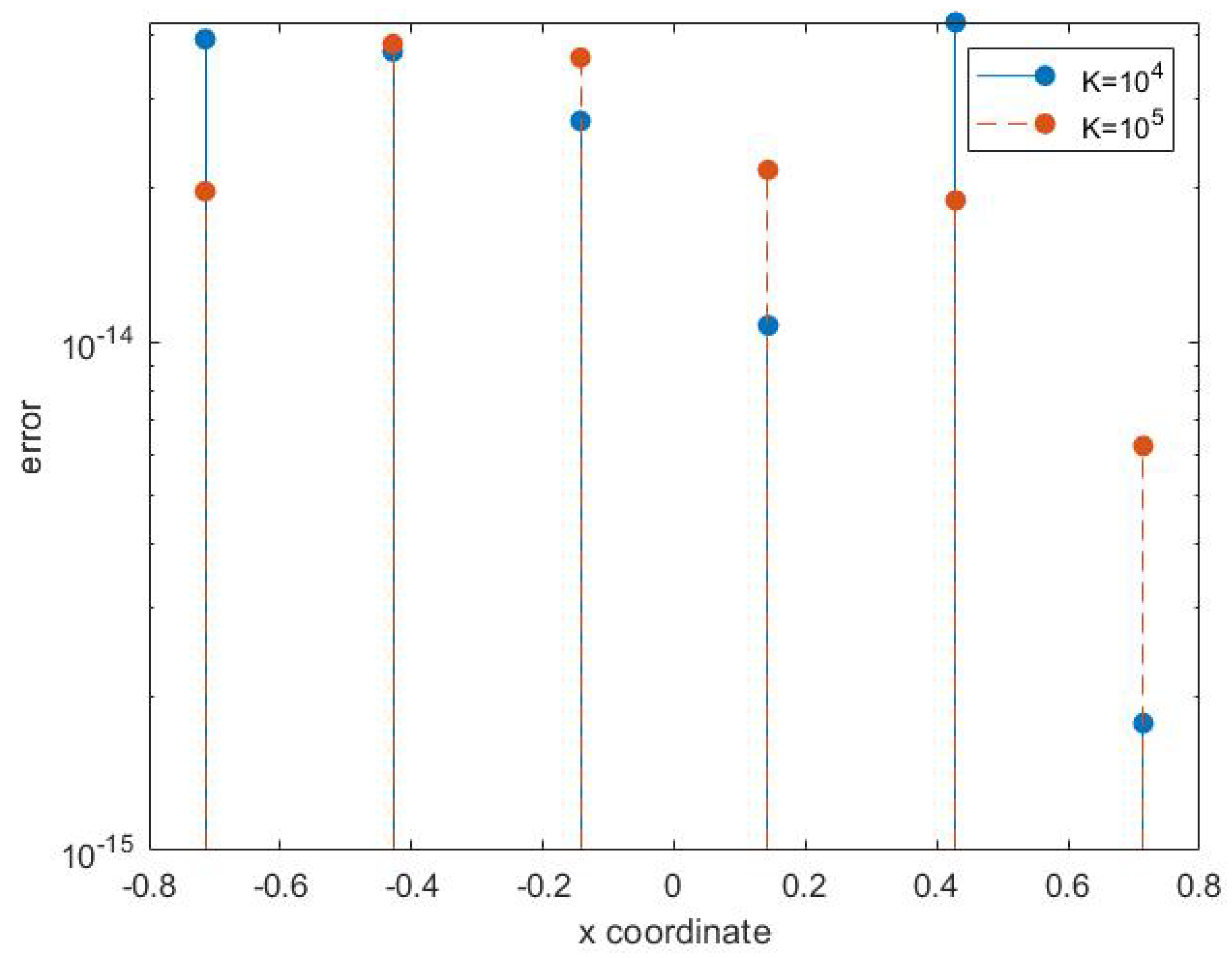
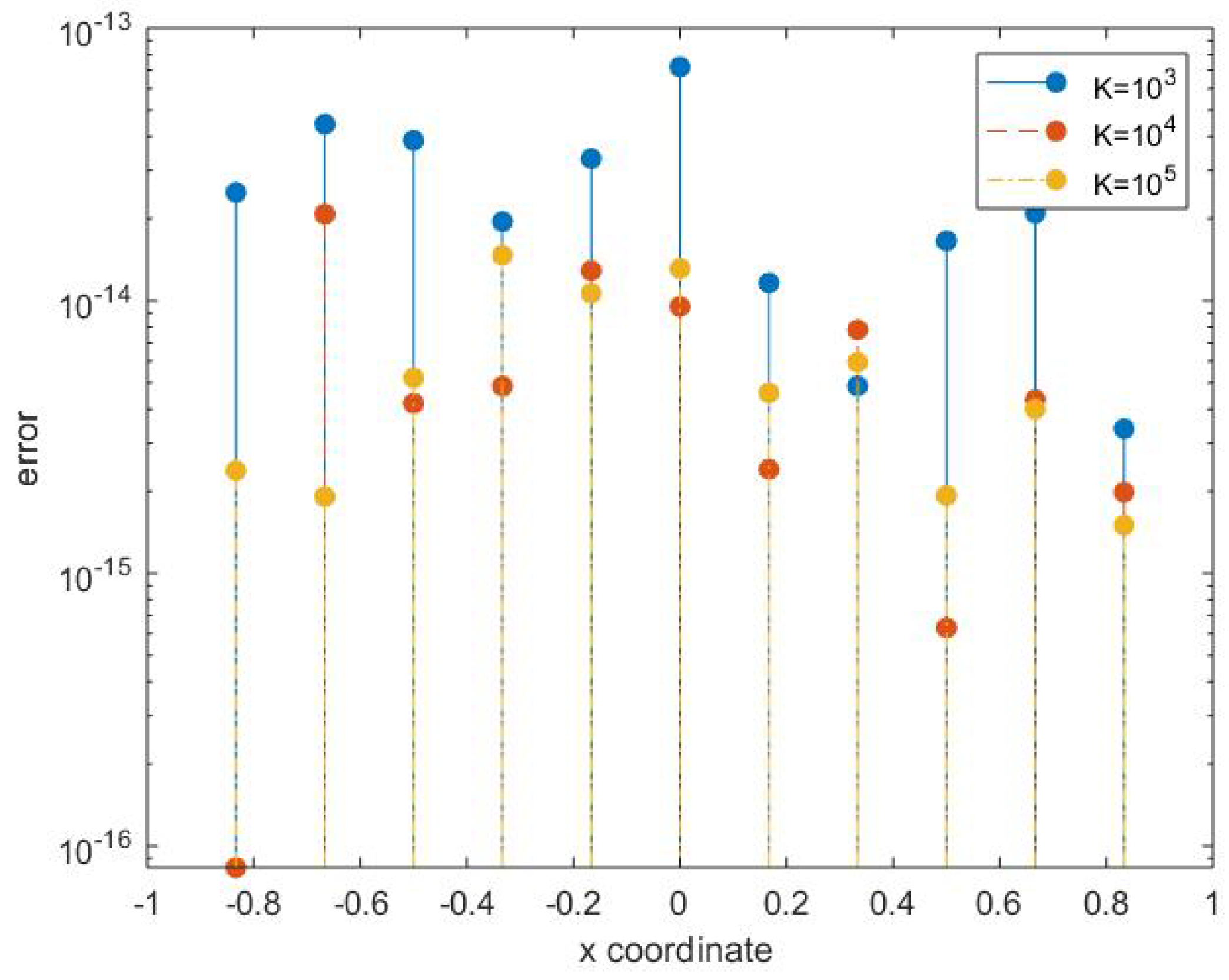
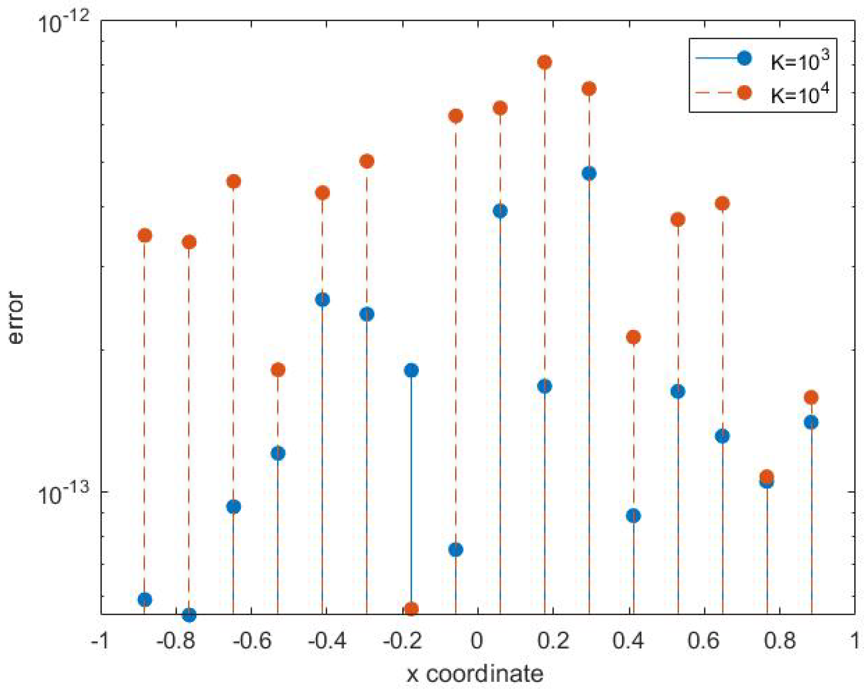
5. Conclusions

In this paper, we have given a really simple but efficient method to solve the highly oscillatory singular FIDEs. For a small number of equally spaced points $x_i,i=0,1,2,\cdots ,N$ as collocation points, the proposed method provides efficient higher accuracy. We do not need to take the higher $mth$ degree Taylor series expansion of the Chebyshev polynomial, as even for $m=1$ we obtain satisfactory approximation to the exact values. However, for weak singularities, the $w\left(t\right)\ne 1$ values of m and N are taken to be identical. All the exact values of the integrals are calculated in Mathematica11 software, whereas the code for the proposed method is developed in MatlabR2018a.