Dispersive Optical Solitons to Stochastic Resonant NLSE with Both Spatio-Temporal and Inter-Modal Dispersions Having Multiplicative White Noise

Abstract

The current article studies optical solitons solutions for the dimensionless form of the stochastic resonant nonlinear Schrödinger equation (NLSE) with both spatio-temporal dispersion (STD) and inter-modal dispersion (IMD) having multiplicative noise in the itô sense. We will discuss seven laws of nonlinearities, namely, the Kerr law, power law, parabolic law, dual-power law, quadratic–cubic law, polynomial law, and triple-power law. The new auxiliary equation method is investigated. We secure the bright, dark, and singular soliton solutions for the model.

1. Introduction

The stochastic nonlinear differential equations which contain the stochastic term with multiplicative noise play an essential role in scientific fields and engineering. One of these models’ fundamental physical problems is getting their soliton solutions. The search for mathematical techniques to deduce exact solutions for these equations is a fundamental action. It is well known that the resonant nonlinear Schrödinger equation (NLSE) comprises the nonlinear dynamics of optical solitons and Madelung fluids. Generally, in the quantum Hall effect, we take into consideration the study of chiral solitons in a specific resonant term in (1 + 1) dimensions [1,2,3,4,5,6,7,8] and in (2 + 1) dimensions [9]. Recently, many papers have deduced the exact solitons solutions for nonlinear partial differential equations (NLPDEs) by using different methods. Namely, Hirota bilinear method [10], physical information neural network (PINN) method [11], Riccati equation expansion method, and Jacobian elliptic equation expansion method [12], semi-inverse variational principle [13], improved adomian decomposition method [14], undetermined coefficients method [15], modified simple equation scheme, and trial equation approach [16], ansatz approach [17], tanh-coth scheme [18], the mapping method based on a Riccati equation [19], and others. Recently, there are new applications of NLSEs such as, the physical information neural network [20], the waveguide amplifier [21], the breather solutions in different planes [22], the comprehended dynamics of solitary waves in the local case [23], and the anti-interference ability of stable solutions [24]. Recently, a number of articles on stochasticity have been published [25,26,27,28,29,30,31,32,33,34,35].

In the article [36], the authors discussed the wick-type stochastic NLSE using the Hirota method combined with the Hermite transformation; howver, in our present article, we have discussed the stochastic resonant NLSE in the itô sense using the new auxiliary equation method. These two governing models are absolutely different.

The current paper focuses on studying the dimensionless form of the stochastic resonant NLSE with both STD and IMD having multiplicative noise in the itô sense with seven different kinds of nonlinear forms. In the recent corresponding Itô calculus, the soliton solutions will be deduced by using the new auxiliary equation method.

Governing Model

The dimensionless form of the stochastic resonant NLSE with both STD and IMD having multiplicative noise in the itô sense is introduced, for the first time, as

$$\begin{array}{c}i{\mathsf{\Phi }}_t+a{\mathsf{\Phi }}_{xx}+b{\mathsf{\Phi }}_{xt}+F\left({\left|\mathsf{\Phi }\right|}^2\right)\mathsf{\Phi }+\gamma \left({\displaystyle \frac{{\left|\mathsf{\Phi }\right|}_{xx}}{\left|\mathsf{\Phi }\right|}}\right)\mathsf{\Phi }+\sigma \left(\mathsf{\Phi }-ib{\mathsf{\Phi }}_x\right){\displaystyle \frac{dW\left(t\right)}{dt}}=i\delta {\mathsf{\Phi }}_x,\hfill \end{array}$$

(1)

where $\mathsf{\Phi }=\mathsf{\Phi }(x,t)$ is a complex-valued function symbolizes the wave profile, a, b, $\gamma$, $\delta$, and $\sigma$ are real-valued constants with $i=\sqrt{-1}$. The first term of Equation (1) is the linear temporal evolution, also the chromatic dispersion (CD) and STD terms are symbolized by a and b, respectively. Next, $F\left({\left|\mathsf{\Phi }\right|}^2\right)$ is the functional which represents the nonlinearity forms, while $\gamma$ is the coefficient of resonant nonlinearity, and $\delta$ is coefficient of IMD. Finally, $\sigma$ is the coefficient of noise strength and $W\left(t\right)$ is the standard Wiener tactic such that ${\displaystyle \frac{dW\left(t\right)}{dt}}$ is the white noise. Without noise ($\sigma =0$), Equation (1) reduces to the well-known resonant NLSE with both STD and IMD which has been previously studied in [7,8]. The motivation for adding the stochastic term $\sigma \left(\mathsf{\Phi }-ib{\mathsf{\Phi }}_x\right){\displaystyle \frac{dW\left(t\right)}{dt}}$ to Equation (1) is to formulate the stochastic differential equation with noise or fluctuations depending on the time, which has been recognized in many areas via physics, engineering, biology, chemistry, and so on.

The purpose of the present paper is to derive bright, dark, and singular soliton solutions for Equation (1) with seven various forms of nonlinearity, namely, Kerr law, power law, parabolic law, dual-power law, quadratic-cubic law, polynomial law, and triple-power law by using the new auxiliary equation technique.

In Section 2, we will construct the mathematical analysis for Equation (1). In Section 3, Section 4, Section 5, Section 6, Section 7, Section 8 and Section 9, we will establish seven laws of nonlinearities mentioned above for Equation (1) and solving them by using the new auxiliary equation method. In Section 10, conclusions will be presented.

2. Mathematical Analysis

In order to solve the stochastic Equation (1), we use a wave transformation involving the noise coefficient $\sigma$ and the Wiener process $W\left(t\right)$ in the form

$$\mathsf{\Phi }(x,t)=g\left(z\right)e^{i\left[-\kappa x+\omega t+\sigma W\left(t\right)-{\sigma }^{2}t\right]},$$

(2)

and

$$z=x-vt,$$

(3)

where $\kappa ,\omega$, and v are real constants. Thus, the real function $g\left(z\right)$ represents the pulse shape, while $\kappa ,\omega$, and v symbolize to soliton frequency, wave number and soliton velocity, respectively. Inserting (2) and (3) in Equation (1), one deduces

$$\left(a-bv+\gamma \right)g^{″}+\left[\left(\omega -{\sigma }^2\right)\left(b\kappa -1\right)-a{\kappa }^2-\delta \kappa \right]g+F\left(g^2\right)g=0,$$

(4)

and

$$\left[-v-2a\kappa +b\kappa v+b\left(\omega -{\sigma }^2\right)-\delta \right]g^{\prime }=0.$$

(5)

which represent the real and imaginary parts, respectively. From Equation (5), the soliton velocity is obtained as

$$v=\frac{b\left(\omega -{\sigma }^2\right)-2a\kappa -\delta }{1-b\kappa },$$

(6)

provided

$$b\kappa \ne 1.$$

(7)

In the next sections, we will solve Equation (4) when $F\left({\mathsf{\Phi }}^2\right)$ takes seven forms of nonlinearities.

3. Kerr Law

To this end, the nonlinearity form of the Kerr law is specified by

$$F\left(g^2\right)=c{g}^2,$$

(8)

such that c is a non-zero constant. Equation (1) using (8) becomes

$$\begin{array}{c}i{\mathsf{\Phi }}_t+a{\mathsf{\Phi }}_{xx}+b{\mathsf{\Phi }}_{xt}+c{\left|\mathsf{\Phi }\right|}^2\mathsf{\Phi }+\gamma \left({\displaystyle \frac{{\left|\mathsf{\Phi }\right|}_{xx}}{\left|\mathsf{\Phi }\right|}}\right)\mathsf{\Phi }+\sigma \left(\mathsf{\Phi }-ib{\mathsf{\Phi }}_x\right){\displaystyle \frac{dW\left(t\right)}{dt}}=i\delta {\mathsf{\Phi }}_x,\hfill \end{array}$$

(9)

Thus, Equation (4) takes the form

$$\left(a-bv+\gamma \right)g^{″}+\left[\left(\omega -{\sigma }^2\right)\left(b\kappa -1\right)-a{\kappa }^2-\delta \kappa \right]g+c{g}^3=0.$$

(10)

Now, we will employ the following method to solve Equation (10).

New Auxiliary Equation Approach

To use this method (see [37]), we allow the solution of Equation (10) to be

$$g\left(z\right)=\sum _{m=0}^N{H}_m{Q}^m\left(z\right),$$

(11)

as long as $Q\left(z\right)$ satisfies the ODE

$$Q^{\prime 2}\left(z\right)=\sum _{h=0}^M{r}_h{Q}^h\left(z\right),M⩽8,$$

(12)

where $H_m$ and $r_h$ are constants, such that $H_N\ne 0$, $r_M\ne 0$ and N is the balance number which is determined from the formula

$$D\left[g^j{g}^{\left(l\right)}\right]=N\left(j+1\right)+l\left(\frac{M}{2}-1\right).$$

Set $M=8$, one gets

$$D\left[g^j{g}^{\left(l\right)}\right]=N\left(j+1\right)+3l,$$

(13)

which means $D\left(g\right)=N$, $D\left(g^2\right)=2N$, $D\left(g^{\prime }\right)=N+3$, $D\left(g^{″}\right)=N+6$ and so on.

The current method derives the solutions of Equation (12) as

Family-1. If $r_0=r_1=r_3=r_4=r_6=r_7=0$, $r_2>0,$ then one gets

(I) Bright soliton solutions

$$Q\left(z\right)={\left({\displaystyle \frac{2\epsilon r_2}{\sqrt{r_5^2-4r_2{r}_8}cosh\left(3\sqrt{r_2}z\right)-\epsilon r_5}}\right)}^{\frac{1}{3}},$$

(14)

provided $r_5^2-4r_2{r}_8>0$ and $\epsilon =\pm 1$.

(II) Singular soliton solutions

$$Q\left(z\right)={\left({\displaystyle \frac{2\epsilon r_2}{\sqrt{-\left(r_5^2-4r_2{r}_8\right)}sinh\left(3\sqrt{r_2}z\right)-\epsilon r_5}}\right)}^{\frac{1}{3}},$$

(15)

provided $r_5^2-4r_2{r}_8<0$ and $\epsilon =\pm 1$.

Family-2. If $r_0=r_1=r_3=r_4=r_6=r_7=0$, $r_2>0$ and $r_8={\displaystyle \frac{r_5^2}{4r_2}}$, then one gets

(I) Dark soliton solutions

$$Q\left(z\right)={\left\{-{\displaystyle \frac{r_2}{r_5}}\left[1\pm tanh\left(\frac{3}{2}\sqrt{r_2}z\right)\right]\right\}}^{\frac{1}{3}}.$$

(16)

(II) Singular soliton solutions

$$Q\left(z\right)={\left\{-{\displaystyle \frac{r_2}{r_5}}\left[1\pm coth\left(\frac{3}{2}\sqrt{r_2}z\right)\right]\right\}}^{\frac{1}{3}}.$$

(17)

As a result, by using (13), we balance $g^{″}$ and $g^3$ in Equation (10), to derive $N=3$. Consequently, from (11), the solution of Equation (10) has the form

$$g\left(z\right)=H_0+H_{1}Q\left(z\right)+H_2{Q}^2\left(z\right)+H_3{Q}^3\left(z\right),$$

(18)

where $H_m(m=0,1,2,3)$ are constants and $H_3\ne 0$. Substituting (18) and (12) with $M=8$ into Equation (10), one derives the following algebraic equations,

$$\left.\begin{array}{c}18\left(a-bv+\gamma \right)H_3{r}_8+c{H}_3^3=0,\hfill \\ \\ 20\left(a-bv+\gamma \right)H_2{r}_8+6c{H}_2{H}_3^2+33\left(a-bv+\gamma \right)H_3{r}_7=0,\hfill \\ \\ \left(a-bv+\gamma \right)\left[4H_2{r}_0+H_1{r}_1\right]+2c{H}_0^3+2H_0\left[\left(\omega -{\sigma }^2\right)\left(b\kappa -1\right)-a{\kappa }^2-\delta \kappa \right]=0,\hfill \\ \\ 3c{H}_2^2{H}_3+\left(a-bv+\gamma \right)\left(4H_1{r}_8+9H_2{r}_7+15H_3{r}_6\right)+3c{H}_1{H}_3^2=0,\hfill \\ \\ 3c{H}_0^2{H}_1+\left(a-bv+\gamma \right)\left(6H_3{r}_0+3H_2{r}_1+H_1{r}_2\right)+\left[\left(\omega -{\sigma }^2\right)\left(b\kappa -1\right)-a{\kappa }^2-\delta \kappa \right]H_1=0,\hfill \\ \\ 3\left(a-bv+\gamma \right)H_1{r}_3+15\left(a-bv+\gamma \right)H_3{r}_1+6c{H}_0{H}_1^2+6c{H}_0^2{H}_2\hfill \\ +2\left[\left(\omega -{\sigma }^2\right)\left(b\kappa -1\right)-a{\kappa }^2-\delta \kappa \right]H_2+8\left(a-bv+\gamma \right)H_2{r}_2=0,\hfill \\ \\ 3c{H}_1^2{H}_3+\left[12H_3{r}_4+7H_2{r}_{5}3H_1{r}_6\right]\left(a-bv+\gamma \right)+3c{H}_1{H}_2^2+6c{H}_0{H}_2{H}_3=0,\hfill \\ \\ 6c{H}_0{H}_3^2+2c{H}_2^3+\left[7H_1{r}_7+27H_3{r}_5+16H_2{r}_6\right]\left(a-bv+\gamma \right)+12c{H}_1{H}_2{H}_3=0,\hfill \\ \\ 12c{H}_0{H}_1{H}_3+6c{H}_1^2{H}_2+6c{H}_0{H}_2^2+\left[5H_1{r}_5+12H_2{r}_4+21H_3{r}_3\right]\left(a-bv+\gamma \right)=0,\hfill \\ \\ \left[\left(\omega -{\sigma }^2\right)\left(b\kappa -1\right)-a{\kappa }^2-\delta \kappa \right]H_3+\left(5H_2{r}_3+9H_3{r}_2\right)\left(a-bv+\gamma \right)+c{H}_1^3+6c{H}_0{H}_1{H}_2\hfill \\ +3c{H}_0^2{H}_3+2\left(a-bv+\gamma \right)H_1{r}_4=0.\hfill \end{array}\right\}$$

(19)

Thus, we utilize the following types of solutions:

Type-1. Set $r_0=r_1=r_3=r_4=r_6=r_7=0$, in Equation (19) and solving them by using the Maple, one secures

$$H_0=0,H_1=0,H_2=0,H_3=3\sqrt{-\frac{2\left(a-bv+\gamma \right)r_8}{c}},r_2=-\frac{\left(\omega -{\sigma }^2\right)\left(b\kappa -1\right)-a{\kappa }^2-\delta \kappa }{9\left(a-bv+\gamma \right)},r_5=0,r_8=r_8,$$

(20)

provided $c\left(a-bv+\gamma \right)r_8<0.$ Consequently, inserting (20) along with (14) and (15) into Equation (18), one deduces the solutions of Equation (9) as

(I) Bright soliton solutions

$$\mathsf{\Phi }(x,t)=\pm \sqrt{-\frac{2\left[\left(\omega -{\sigma }^2\right)\left(b\kappa -1\right)-a{\kappa }^2-\delta \kappa \right]}{c}}\mathrm{sech}\left[\sqrt{-\frac{\left(\omega -{\sigma }^2\right)\left(b\kappa -1\right)-a{\kappa }^2-\delta \kappa }{a-bv+\gamma }}\left(x-vt\right)\right]e^{i\left[-\kappa x+\omega t+\sigma W\left(t\right)-{\sigma }^{2}t\right]},$$

(21)

provided $\left[\left(\omega -{\sigma }^2\right)\left(b\kappa -1\right)-a{\kappa }^2-\delta \kappa \right]c<0$ and $\left(a-bv+\gamma \right)\left[\left(\omega -{\sigma }^2\right)\left(b\kappa -1\right)-a{\kappa }^2-\delta \kappa \right]<0$. (see Figure 1)

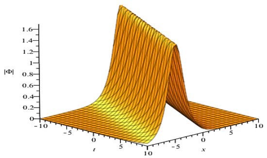
Figure 1. Plot of the bright soliton solution (21) with $a=0.2$, $b=0.35$, $c=0.4$, $\delta =0.5$, $\kappa =0.25$, $\omega =0.6$, $\sigma =0.35$, $v=-0.4743835616$, $\gamma =0.5$, and $-10\le x,t\le 10$.

(II) Singular soliton solutions

$$\mathsf{\Phi }(x,t)=\pm \sqrt{\frac{2\left[\left(\omega -{\sigma }^2\right)\left(b\kappa -1\right)-a{\kappa }^2-\delta \kappa \right]}{c}}\mathrm{csch}\left[\sqrt{-\frac{\left[\left(\omega -{\sigma }^2\right)\left(b\kappa -1\right)-a{\kappa }^2-\delta \kappa \right]}{a-bv+\gamma }}\left(x-vt\right)\right]e^{i\left[-\kappa x+\omega t+\sigma W\left(t\right)-{\sigma }^{2}t\right]},$$

(22)

provided $\left[\left(\omega -{\sigma }^2\right)\left(b\kappa -1\right)-a{\kappa }^2-\delta \kappa \right]c>0$ and $\left(a-bv+\gamma \right)\left[\left(\omega -{\sigma }^2\right)\left(b\kappa -1\right)-a{\kappa }^2-\delta \kappa \right]<0$. (see Figure 2)

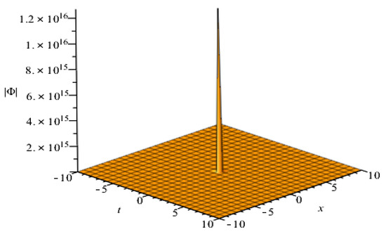
Figure 2. Plot of the singular soliton solution (22) with $a=0.2$, $b=0.35$, $c=-0.4$, $\delta =0.5$, $\kappa =0.25$, $\omega =0.6$, $\sigma =0.35$, $v=-0.4743835616$, $\gamma =0.5$, and $-10\le x,t\le 10.$

Type-2. Set $r_0=r_1=r_3=r_4=r_6=r_7=0$ and $r_8=\frac{r_5^2}{4r_2}$, in Equation (19) and solving them by using the Maple, one obtains

$$\begin{array}{c}{E}_0=\sqrt{-\frac{\left(\omega -{\sigma }^2\right)\left(b\kappa -1\right)-a{\kappa }^2-\delta \kappa }{c}},E_1=0,E_2=0,E_3=\frac{9r_5\left(a-bv+\gamma \right)}{2\left[\left(\omega -{\sigma }^2\right)\left(b\kappa -1\right)-a{\kappa }^2-\delta \kappa \right]}\sqrt{-\frac{\left(\omega -{\sigma }^2\right)\left(b\kappa -1\right)-a{\kappa }^2-\delta \kappa }{c}},\\ \\ r_2=\frac{2\left[\left(\omega -{\sigma }^2\right)\left(b\kappa -1\right)-a{\kappa }^2-\delta \kappa \right]}{9\left(a-bv+\gamma \right)},r_5=r_5,\end{array}$$

(23)

provided $c\left[\left(\omega -{\sigma }^2\right)\left(b\kappa -1\right)-a{\kappa }^2-\delta \kappa \right]<0$ and $\left(a-bv+\gamma \right)\ne 0$. Consequently, inserting (23) along with (16) and (17) into Equation (18), one deduces the solutions of Equation (9) as

(I) Dark soliton solutions (see Figure 3)

$$\mathsf{\Phi }(x,t)=\pm \sqrt{-\frac{\left(\omega -{\sigma }^2\right)\left(b\kappa -1\right)-a{\kappa }^2-\delta \kappa }{c}}tanh\left[\sqrt{\frac{\left(\omega -{\sigma }^2\right)\left(b\kappa -1\right)-a{\kappa }^2-\delta \kappa }{2\left(a-bv+\gamma \right)}}\left(x-vt\right)\right]e^{i\left[-\kappa x+\omega t+\sigma W\left(t\right)-{\sigma }^{2}t\right]},$$

(24)

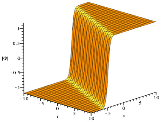
Figure 3. Plot of the dark soliton solution (24) with $a=0.2$, $b=0.35$, $c=0.4$, $\delta =0.5$, $\kappa =0.25$, $\omega =0.6$, $\sigma =0.35$, $v=-0.4743835616$, $\gamma =-0.5$, and $-10\le x,t\le 10.$

(II) Singular soliton solutions (see Figure 4)

$$\mathsf{\Phi }(x,t)=\pm \sqrt{-\frac{\left(\omega -{\sigma }^2\right)\left(b\kappa -1\right)-a{\kappa }^2-\delta \kappa }{c}}coth\left[\sqrt{\frac{\left(\omega -{\sigma }^2\right)\left(b\kappa -1\right)-a{\kappa }^2-\delta \kappa }{2\left(a-bv+\gamma \right)}}\left(x-vt\right)\right]e^{i\left[-\kappa x+\omega t+\sigma W\left(t\right)-{\sigma }^{2}t\right]},$$

(25)

provided $c\left[\left(\omega -{\sigma }^2\right)\left(b\kappa -1\right)-a{\kappa }^2-\delta \kappa \right]<0$ and $\left(a-bv+\gamma \right)\left[\left(\omega -{\sigma }^2\right)\left(b\kappa -1\right)-a{\kappa }^2-\delta \kappa \right]>0.$

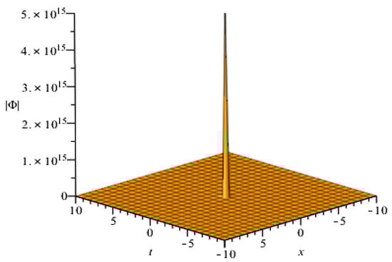
Figure 4. Plot of the singular soliton solution (25) with $a=0.2$, $b=0.35$, $c=0.4$, $\delta =0.5$, $\kappa =0.25$, $\omega =0.6$, $\sigma =0.35$, $v=-0.4743835616$, $\gamma =-0.5$, and $-10\le x,t\le 10.$

4. Power Law

To this aim, the nonlinearity form of the power law is specified by

$$F\left(g^2\right)=c{g}^{2n},$$

(26)

such that c is a non-zero constant and n is the power nonlinearity parameter. Equation (1) using (26) becomes

$$\begin{array}{c}i{\mathsf{\Phi }}_t+a{\mathsf{\Phi }}_{xx}+b{\mathsf{\Phi }}_{xt}+c{\left|\mathsf{\Phi }\right|}^{2n}\mathsf{\Phi }+\gamma \left({\displaystyle \frac{{\left|\mathsf{\Phi }\right|}_{xx}}{\left|\mathsf{\Phi }\right|}}\right)\mathsf{\Phi }+\sigma \left(\mathsf{\Phi }-ib{\mathsf{\Phi }}_x\right){\displaystyle \frac{dW\left(t\right)}{dt}}=i\delta {\mathsf{\Phi }}_x,\hfill \end{array}$$

(27)

Thus, Equation (4) takes the form

$$\left(a-bv+\gamma \right)g^{″}+\left[\left(\omega -{\sigma }^2\right)\left(b\kappa -1\right)-a{\kappa }^2-\delta \kappa \right]g+c{g}^{2n+1}=0.$$

(28)

By using (13), we balancing $g^{″}$ and $g^{2n+1}$ in Equation (28), to derive $N=\frac{3}{n}$. Since N is not integer, then one takes

$$g\left(z\right)={\left[\phi \left(z\right)\right]}^{\frac{3}{n}},$$

(29)

as long as $\phi \left(z\right)>0.$ Inserting (29) into Equation (28) obtains

$$3\left(a-bv+\gamma \right)\left[n\phi {\phi }^{″}+\left(3-n\right){\phi }^{\prime 2}\right]+n^2\left[\left(\omega -{\sigma }^2\right)\left(b\kappa -1\right)-a{\kappa }^2-\delta \kappa \right]{\phi }^2+n^{2}c{\phi }^8=0.$$

(30)

Now, we will employ the following method to solve Equation (30).

New Auxiliary Equation Approach

As a result, by using (13), we balance $\phi {\phi }^{″}$ and ${\phi }^8$ in Equation (30), deriving $N=1$. Consequently, from (11), the solution of Equation (30) has the form

$$\phi \left(z\right)=H_0+H_{1}Q\left(z\right),$$

(31)

where $H_m(m=0,1)$ are constants and $H_1\ne 0$. Substituting (31) and (12) with $M=8$ into Equation (30), one derives the following algebraic equations,

$$\left.\begin{array}{c}c{n}^2{H}_1^8+9\left(n+1\right)\left(a-bv+\gamma \right)H_1^2{r}_8=0,\hfill \\ \\ 16c{n}^2{H}_0{H}_1^7+\left[3\left(5n+3\right)H_1^2{r}_7+12H_{1}n{H}_0{r}_8\right]\left(a-bv+\gamma \right)=0,\hfill \\ \\ 112c{n}^2{H}_0^5{H}_1^3+\left[3\left(n+6\right)H_1^2{r}_3+12H_{1}n{H}_0{r}_4\right]\left(a-bv+\gamma \right)=0,\hfill \\ \\ 3\left(a-bv+\gamma \right)\left[H_1^2{r}_4\left(n+3\right)+5H_{1}n{H}_0{r}_5\right]+140c{n}^2{H}_0^4{H}_1^4=0,\hfill \\ \\ \left[9H_{1}n{H}_0{r}_3+18H_1^2{r}_2\right]\left(a-bv+\gamma \right)+\left[\left(\omega -{\sigma }^2\right)\left(b\kappa -1\right)-a{\kappa }^2-\delta \kappa \right]n^2{H}_1^2+28c{n}^2{H}_0^6{H}_1^2=0,\hfill \\ \\ 112c{n}^2{H}_0^3{H}_1^5+\left[9H_1^{2}n{r}_5+18H_{1}n{H}_0{r}_6+18H_1^2{r}_5\right]\left(a-bv+\gamma \right)=0,\hfill \\ \\ 56c{n}^2{H}_0^2{H}_1^6+\left[21H_{1}n{H}_0{r}_7+12H_1^{2}n{r}_6+18H_1^2{r}_6\right]\left(a-bv+\gamma \right)=0,\hfill \\ \\ 2\left[\left(\omega -{\sigma }^2\right)\left(b\kappa -1\right)-a{\kappa }^2-\delta \kappa +c{H}_0^6\right]n^2{H}_0^2+\left[6H_1^2{r}_0\left(3-n\right)+3H_{1}n{H}_0{r}_1\right]\left(a-bv+\gamma \right)=0,\hfill \\ \\ 3H_1\left[2n{H}_0{r}_2+\left(6-n\right)H_1{r}_1\right]\left(a-bv+\gamma \right)+4n^2{H}_0{H}_1\left[\left(\omega -{\sigma }^2\right)\left(b\kappa -1\right)-a{\kappa }^2-\delta \kappa +4c{H}_0^6\right]=0.\hfill \end{array}\right\}$$

(32)

Thus, we utilize the following type of solutions:

Type-1. Set $r_0=r_1=r_3=r_4=r_6=r_7=0$, in Equation (32) and, solving them by using the Maple, obtaining

$$H_0=0,H_1={\left[-\frac{9\left(n+1\right)\left(a-bv+\gamma \right)r_8}{n^{2}c}\right]}^{\frac{1}{6}},r_2=-\frac{n^2\left[\left(\omega -{\sigma }^2\right)\left(b\kappa -1\right)-a{\kappa }^2-\delta \kappa \right]}{9\left(a-bv+\gamma \right)},r_5=0,r_8=r_8,$$

(33)

provided $c\left(a-bv+\gamma \right)r_8<0.$ Consequently, inserting (33) along with (14) and (15) into Equation (31), one deduces the solutions of Equation (27) as

(I) Bright soliton solutions

$$\mathsf{\Phi }(x,t)={\left\{\pm \sqrt{-\frac{(n+1)\left[\left(\omega -{\sigma }^2\right)\left(b\kappa -1\right)-a{\kappa }^2-\delta \kappa \right]}{c}}\mathrm{sech}\left[n\sqrt{-\frac{\left(\omega -{\sigma }^2\right)\left(b\kappa -1\right)-a{\kappa }^2-\delta \kappa }{\left(a-bv+\gamma \right)}}\left(x-vt\right)\right]\right\}}^{\frac{1}{n}}{e}^{i\left[-\kappa x+\omega t+\sigma W\left(t\right)-{\sigma }^{2}t\right]},$$

(34)

provided $\left[\left(\omega -{\sigma }^2\right)\left(b\kappa -1\right)-a{\kappa }^2-\delta \kappa \right]c<0$ and $\left(a-bv+\gamma \right)\left[\left(\omega -{\sigma }^2\right)\left(b\kappa -1\right)-a{\kappa }^2-\delta \kappa \right]<0.$

(II) Singular soliton solutions

$$\mathsf{\Phi }(x,t)={\left\{\pm \sqrt{\frac{(n+1)\left[\left(\omega -{\sigma }^2\right)\left(b\kappa -1\right)-a{\kappa }^2-\delta \kappa \right]}{c}}\mathrm{csch}\left[n\sqrt{-\frac{\left(\omega -{\sigma }^2\right)\left(b\kappa -1\right)-a{\kappa }^2-\delta \kappa }{\left(a-bv+\gamma \right)}}\left(x-vt\right)\right]\right\}}^{\frac{1}{n}}{e}^{i\left[-\kappa x+\omega t+\sigma W\left(t\right)-{\sigma }^{2}t\right]},$$

(35)

provided $\left[\left(\omega -{\sigma }^2\right)\left(b\kappa -1\right)-a{\kappa }^2-\delta \kappa \right]c>0$ and $\left(a-bv+\gamma \right)\left[\left(\omega -{\sigma }^2\right)\left(b\kappa -1\right)-a{\kappa }^2-\delta \kappa \right]<0.$

5. Parabolic Law

To this aim, the nonlinearity form of the parabolic law is specified by

$$F\left(g^2\right)=c_1{g}^2+c_2{g}^4,$$

(36)

where $c_1$ and $c_2$ are constants and $c_2\ne 0$. Equation (1) using (36) becomes

$$\begin{array}{c}i{\mathsf{\Phi }}_t+a{\mathsf{\Phi }}_{xx}+b{\mathsf{\Phi }}_{xt}+\left(c_1{\left|\mathsf{\Phi }\right|}^2+c_2{\left|\mathsf{\Phi }\right|}^4\right)\mathsf{\Phi }+\gamma \left({\displaystyle \frac{{\left|\mathsf{\Phi }\right|}_{xx}}{\left|\mathsf{\Phi }\right|}}\right)\mathsf{\Phi }+\sigma \left(\mathsf{\Phi }-ib{\mathsf{\Phi }}_x\right){\displaystyle \frac{dW\left(t\right)}{dt}}=i\delta {\mathsf{\Phi }}_x,\hfill \end{array}$$

(37)

Thus, Equation (4) takes the form

$$\left(a-bv+\gamma \right)g^{″}+\left[\left(\omega -{\sigma }^2\right)\left(b\kappa -1\right)-a{\kappa }^2-\delta \kappa \right]g+c_1{g}^3+c_2{g}^5=0.$$

(38)

By using (13), we balancing $g^{″}$ and $g^5$ in Equation (38), to derive $N=\frac{3}{2}$. Since N is not integer, one then takes

$$g\left(z\right)={\left[\phi \left(z\right)\right]}^{\frac{3}{2}},$$

(39)

as long as $\phi \left(z\right)>0.$ Inserting (39) into Equation (38) obtains

$$3\left(a-bv+\gamma \right)\left[2\phi {\phi }^{″}+{\phi }^{\prime 2}\right]+4\left[\left(\omega -{\sigma }^2\right)\left(b\kappa -1\right)-a{\kappa }^2-\delta \kappa \right]{\phi }^2+4c_1{\phi }^5+4c_2{\phi }^8=0.$$

(40)

Next, we employ the following method to solve Equation (40).

New Auxiliary Equation Approach

As a result, by using (13), we balance $\phi {\phi }^{″}$ and ${\phi }^8$ in Equation (40), to get $N=1$. Consequently, from (11), the solution of Equation (40) has the same form (31). Substituting (31) and (12) with $M=8$ into Equation (40), one derives the following algebraic equations,

$$\left.\begin{array}{c}4c_2{H}_1^8+27\left(a-bv+\gamma \right)H_1^2{r}_8=0,\hfill \\ \\ 21\left(a-bv+\gamma \right)\left(H_1^2{r}_6+H_1{H}_0{r}_7\right)+112c_2{H}_0^2{H}_1^6=0,\hfill \\ \\ 32c_2{H}_0{H}_1^7+24\left(a-bv+\gamma \right)\left(H_1{H}_0{r}_8+H_1^2{r}_7\right)=0,\hfill \\ \\ 18\left(a-bv+\gamma \right)\left(H_1^2{r}_5+H_1{H}_0{r}_6\right)+224c_2{H}_0^3{H}_1^5+4c_1{H}_1^5=0,\hfill \\ \\ 20c_1{H}_0{H}_1^4+280c_2{H}_0^4{H}_1^4+15\left(a-bv+\gamma \right)\left(H_1{H}_0{r}_5+H_1^2{r}_4\right)=0,\hfill \\ \\ 40c_1{H}_0^2{H}_1^3+224c_2{H}_0^5{H}_1^3+12\left(a-bv+\gamma \right)\left(H_1^2{r}_3+12H_1{H}_0{r}_4\right)=0,\hfill \\ \\ 6\left(a-bv+\gamma \right)\left(H_1^2{r}_1+H_1{H}_0{r}_2\right)+20c_1{H}_0^4{H}_1+8\left[\left(\omega -{\sigma }^2\right)\left(b\kappa -1\right)-a{\kappa }^2-\delta \kappa \right]H_0{H}_1+32c_2{H}_0^7{H}_1=0,\hfill \\ \\ 40c_1{H}_0^3{H}_1^2+4\left[\left(\omega -{\sigma }^2\right)\left(b\kappa -1\right)-a{\kappa }^2-\delta \kappa \right]H_1^2+112c_2{H}_0^6{H}_1^2+9\left(H_1^2{r}_2+H_1{H}_0{r}_3\right)\left(a-bv+\gamma \right)=0,\hfill \\ \\ 3\left(a-bv+\gamma \right)\left(H_1{H}_0{r}_1+H_1^2{r}_0\right)+4\left[\left(\omega -{\sigma }^2\right)\left(b\kappa -1\right)-a{\kappa }^2-\delta \kappa \right]H_0^2+4c_1{H}_0^5+4c_2{H}_0^8=0\hfill \end{array}\right\}$$

(41)

Thus, we utilize the following types of solutions:

Type-1. Set $r_0=r_1=r_3=r_4=r_6=r_7=0$, in Equation (41) and solving them by using the Maple, one obtains

$$H_0=0,H_1={\left[-\frac{27\left(a-bv+\gamma \right)r_8}{4c_2}\right]}^{\frac{1}{6}},r_2=-\frac{4\left[\left(\omega -{\sigma }^2\right)\left(b\kappa -1\right)-a{\kappa }^2-\delta \kappa \right]}{9\left(a-bv+\gamma \right)},r_5=-\frac{c_1}{\left(a-bv+\gamma \right)}\sqrt{-\frac{\left(a-bv+\gamma \right)r_8}{3c_2}},r_8=r_8,$$

(42)

provided $c_2\left(a-bv+\gamma \right)r_8<0.$ Consequently, inserting (42) along with (14) and (15) into Equation (31), one deduces the solutions of Equation (37) as

(I) Bright soliton solutions

$$\mathsf{\Phi }(x,t)={\left\{\frac{12\left[\left(\omega -{\sigma }^2\right)\left(b\kappa -1\right)-a{\kappa }^2-\delta \kappa \right]}{\pm \sqrt{9c_1^2-48c_2\left[\left(\omega -{\sigma }^2\right)\left(b\kappa -1\right)-a{\kappa }^2-\delta \kappa \right]}cosh\left[2\sqrt{-\frac{\left(\omega -{\sigma }^2\right)\left(b\kappa -1\right)-a{\kappa }^2-\delta \kappa }{\left(a-bv+\gamma \right)}}\left(x-vt\right)\right]-3c_1}\right\}}^{\frac{1}{2}}{e}^{i\left[-\kappa x+\omega t+\sigma W\left(t\right)-{\sigma }^{2}t\right]},$$

(43)

provided $9c_1^2-48c_2[(\omega -{\sigma }^2)(b\kappa -1)-a{\kappa }^2-\delta \kappa ]>0$ and $(a-bv+\gamma )[(\omega -{\sigma }^2)(b\kappa -1)-a{\kappa }^2-\delta \kappa ]<0.$

(II) Singular soliton solutions

$$\mathsf{\Phi }(x,t)={\left\{\frac{12\left[\left(\omega -{\sigma }^2\right)\left(b\kappa -1\right)-a{\kappa }^2-\delta \kappa \right]}{\pm \sqrt{-\left(9c_1^2-48c_2\left[\left(\omega -{\sigma }^2\right)\left(b\kappa -1\right)-a{\kappa }^2-\delta \kappa \right]\right)}sinh\left[2\sqrt{-\frac{\left(\omega -{\sigma }^2\right)\left(b\kappa -1\right)-a{\kappa }^2-\delta \kappa }{\left(a-bv+\gamma \right)}}\left(x-vt\right)\right]-3c_1}\right\}}^{\frac{1}{2}}{e}^{i\left[-\kappa x+\omega t+\sigma W\left(t\right)-{\sigma }^{2}t\right]},$$

(44)

provided $9c_1^2-48c_2[(\omega -{\sigma }^2)(b\kappa -1)-a{\kappa }^2-\delta \kappa ]<0$ and $(a-bv+\gamma )[(\omega -{\sigma }^2)(b\kappa -1)-a{\kappa }^2-\delta \kappa ]<0.$

Type-2. Set $r_0=r_1=r_3=r_4=r_6=r_7=0$ and $r_8=\frac{r_5^2}{4r_2}$, in Equation (41) and solving them by using the Maple, one obtains

$$H_0=0,H_1={\left[\frac{243{\left(a-bv+\gamma \right)}^2{r}_5^2}{64c_2\left[\left(\omega -{\sigma }^2\right)\left(b\kappa -1\right)-a{\kappa }^2-\delta \kappa \right]}\right]}^{\frac{1}{6}},r_2=-\frac{4\left[\left(\omega -{\sigma }^2\right)\left(b\kappa -1\right)-a{\kappa }^2-\delta \kappa \right]}{9\left(a-bv+\gamma \right)},r_5=r_5,$$

(45)

and

$$c_1=-4c_2\sqrt{\frac{\left(\omega -{\sigma }^2\right)\left(b\kappa -1\right)-a{\kappa }^2-\delta \kappa }{3c_2}},$$

(46)

provided $c_2\left[\left(\omega -{\sigma }^2\right)\left(b\kappa -1\right)-a{\kappa }^2-\delta \kappa \right]>0$ and $\left(a-bv+\gamma \right)\ne 0$. Consequently, inserting (45) along with (16) and (17) into Equation (31), one deduces the solutions of Equation (37) as:

(I) Dark soliton solution

$$\mathsf{\Phi }(x,t)={\left\{\frac{1}{2}\sqrt{\frac{3\left[\left(\omega -{\sigma }^2\right)\left(b\kappa -1\right)-a{\kappa }^2-\delta \kappa \right]}{c_2}}\left(1+tanh\left[\sqrt{-\frac{\left(\omega -{\sigma }^2\right)\left(b\kappa -1\right)-a{\kappa }^2-\delta \kappa }{a-bv+\gamma }}\left(x-vt\right)\right]\right)\right\}}^{\frac{1}{2}}{e}^{i\left[-\kappa x+\omega t+\sigma W\left(t\right)-{\sigma }^{2}t\right]},$$

(47)

(II) Singular soliton solution

$$\mathsf{\Phi }(x,t)={\left\{\frac{1}{2}\sqrt{\frac{3\left[\left(\omega -{\sigma }^2\right)\left(b\kappa -1\right)-a{\kappa }^2-\delta \kappa \right]}{c_2}}\left(1+coth\left[\sqrt{-\frac{\left(\omega -{\sigma }^2\right)\left(b\kappa -1\right)-a{\kappa }^2-\delta \kappa }{a-bv+\gamma }}\left(x-vt\right)\right]\right)\right\}}^{\frac{1}{2}}{e}^{i\left[-\kappa x+\omega t+\sigma W\left(t\right)-{\sigma }^{2}t\right]},$$

(48)

provided $c_2[(\omega -{\sigma }^2)(b\kappa -1)-a{\kappa }^2-\delta \kappa ]>0$ and $(a-bv+\gamma )[(\omega -{\sigma }^2)(b\kappa -1)-a{\kappa }^2-\delta \kappa ]<0.$

6. Dual Power Law

To this aim, the nonlinearity form of the dual power law is specified by

$$F\left(g^{2n}\right)=c_1{g}^{2n}+c_2{g}^{4n},$$

(49)

where $c_1$ and $c_2$ are constants and $c_2\ne 0$. Equation (1) using (49) becomes

$$\begin{array}{c}i{\mathsf{\Phi }}_t+a{\mathsf{\Phi }}_{xx}+b{\mathsf{\Phi }}_{xt}+\left(c_1{\left|\mathsf{\Phi }\right|}^{2n}+c_2{\left|\mathsf{\Phi }\right|}^{4n}\right)\mathsf{\Phi }+\gamma \left({\displaystyle \frac{{\left|\mathsf{\Phi }\right|}_{xx}}{\left|\mathsf{\Phi }\right|}}\right)\mathsf{\Phi }+\sigma \left(\mathsf{\Phi }-ib{\mathsf{\Phi }}_x\right){\displaystyle \frac{dW\left(t\right)}{dt}}=i\delta {\mathsf{\Phi }}_x,\hfill \end{array}$$

(50)

Thus, Equation (4) takes the form

$$\left(a-bv+\gamma \right)g^{″}+\left[\left(\omega -{\sigma }^2\right)\left(b\kappa -1\right)-a{\kappa }^2-\delta \kappa \right]g+c_1{g}^{2n+1}+c_2{g}^{4n+1}=0.$$

(51)

By using (13), we balancing $g^{″}$ and $g^{4n+1}$ in Equation (51), to derive $N=\frac{3}{2n}$. Since N is not integer, then one takes

$$g\left(z\right)={\left[\phi \left(z\right)\right]}^{\frac{3}{2n}},$$

(52)

as long as $\phi \left(z\right)>0.$ Inserting (52) into Equation (51) yields

$$3\left(a-bv+\gamma \right)\left[2n\phi {\phi }^{″}+\left(3-2n\right){\phi }^{\prime 2}\right]+4n^2\left[\left(\omega -{\sigma }^2\right)\left(b\kappa -1\right)-a{\kappa }^2-\delta \kappa \right]{\phi }^2+4n^2{c}_1{\phi }^5+4n^2{c}_2{\phi }^8=0.$$

(53)

Next, we will employ the following method to solve Equation (53).

New Auxiliary Equation Approach

As a result, by using (13), we balance $\phi {\phi }^{″}$ and ${\phi }^8$ in Equation (53), to get $N=1$. Consequently, from (11), the solution of Equation (53) has the same form (31). Substituting (31) and (12) with $M=8$ into Equation (53), one derives the following algebraic equations,

$$\left.\begin{array}{c}9\left(a-bv+\gamma \right)\left(2n+1\right)H_1^2{r}_8+4c_2{n}^2{H}_1^8=0,\hfill \\ \\ 3\left(a-bv+\gamma \right)\left[H_1^2{r}_6\left(4n+3\right)+7n{H}_1{H}_0{r}_7\right]+112c_2{n}^2{H}_0^2{H}_1^6=0,\hfill \\ \\ 3\left(a-bv+\gamma \right)\left[H_1^2{r}_7\left(5n+3\right)+8n{H}_1{H}_0{r}_8\right]+32c_2{n}^2{H}_0{H}_1^7=0,\hfill \\ \\ 4\left[\left(\omega -{\sigma }^2\right)\left(b\kappa -1\right)-a{\kappa }^2-\delta \kappa \right]n^2{H}_1^2+\left(a-bv+\gamma \right)\left(9H_1^2{r}_2+9H_{1}n{H}_0{r}_3\right)\hfill \\ +8\left(14c_2{H}_0^3+5c_1\right)n^2{H}_0^3{H}_1^2=0,\hfill \\ \\ 4n^2{H}_1^5\left(c_1+56c_2{H}_0^3\right)+\left(9H_1^2{r}_5+9H_1^{2}n{r}_5+18H_{1}n{H}_0{r}_6\right)\left(a-bv+\gamma \right)=0,\hfill \\ \\ 20n^2{H}_0{H}_1^4\left(14c_2{H}_0^3+c_1\right)+\left(a-bv+\gamma \right)\left[3\left(2n+3\right)H_1^2{r}_4+15n{H}_1{H}_0{r}_5\right]=0,\hfill \\ \\ 224c_2{n}^2{H}_0^5{H}_1^3+40c_1{n}^2{H}_0^2{H}_1^3+\left(3H_1^{2}n{r}_3+12H_{1}n{H}_0{r}_4+9H_1^2{r}_3\right)\left(a-bv+\gamma \right)=0,\hfill \\ \\ +4c_1{n}^2{H}_0^5+4c_2{n}^2{H}_0^8+\left(a-bv+\gamma \right)\left(3H_{1}n{H}_0{r}_1-6H_1^{2}n{r}_0+9H_1^2{r}_0\right)\hfill \\ +4\left[\left(\omega -{\sigma }^2\right)\left(b\kappa -1\right)-a{\kappa }^2-\delta \kappa \right]n^2{H}_0^2=0,\hfill \\ \\ \left[6H_{1}n{H}_0{r}_2+3\left(3-n\right)H_1^2{r}_1\right]\left(a-bv+\gamma \right)+20c_1{n}^2{H}_0^4{H}_1+32c_2{n}^2{H}_0^7{H}_1\hfill \\ +8\left[\left(\omega -{\sigma }^2\right)\left(b\kappa -1\right)-a{\kappa }^2-\delta \kappa \right]n^2{H}_0{H}_1=0.\hfill \end{array}\right\}$$

(54)

Thus, we utilize the following types of solutions:

Type-1. Set $r_0=r_1=r_3=r_4=r_6=r_7=0$, in Equation (54) and solving it by using the Maple, one obtains

$$\begin{array}{c}{H}_0=0,H_1={\left[-\frac{9\left(2n+1\right)\left(a-bv+\gamma \right)r_8}{4n^2{c}_2}\right]}^{\frac{1}{6}},r_2=-\frac{4n^2\left[\left(\omega -{\sigma }^2\right)\left(b\kappa -1\right)-a{\kappa }^2-\delta \kappa \right]}{9\left(a-bv+\gamma \right)},\\ \\ r_5=-\frac{2n{c}_1}{3(1+n)\left(a-bv+\gamma \right)}\sqrt{-\frac{(2n+1)\left(a-bv+\gamma \right)r_8}{c_2}},r_8=r_8,\end{array}$$

(55)

provided $c_2\left(a-bv+\gamma \right)r_8<0.$ Consequently, inserting (55) along with (14) and (15) into Equation (31), one deduces the solutions of Equation (50) as

(I) Bright soliton solutions

$$\begin{array}{c}\mathsf{\Phi }(x,t)={\left\{\frac{2(1+n)(2n+1)\left[\left(\omega -{\sigma }^2\right)\left(b\kappa -1\right)-a{\kappa }^2-\delta \kappa \right]}{\pm \sqrt{{(2n+1)}^2{c}_1^2-4{(1+n)}^2(2n+1)c_2\left[\left(\omega -{\sigma }^2\right)\left(b\kappa -1\right)-a{\kappa }^2-\delta \kappa \right]}cosh\left[2n\sqrt{-\frac{\left(\omega -{\sigma }^2\right)\left(b\kappa -1\right)-a{\kappa }^2-\delta \kappa }{a-bv+\gamma }}\left(x-vt\right)\right]-(2n+1)c_1}\right\}}^{\frac{1}{2n}}\\ \\ \times e^{i\left[-\kappa x+\omega t+\sigma W\left(t\right)-{\sigma }^{2}t\right]},\end{array}$$

(56)

provided $(2n+1)c_1^2-4{(1+n)}^2{c}_2[(\omega -{\sigma }^2)(b\kappa -1)-a{\kappa }^2-\delta \kappa ]>0$ and $(a-bv+\gamma )[(\omega -{\sigma }^2)(b\kappa -1)-a{\kappa }^2-\delta \kappa ]<0.$

(II) Singular soliton solutions

$$\begin{array}{c}\mathsf{\Phi }(x,t)={\left\{\frac{2(1+n)(2n+1)\left[\left(\omega -{\sigma }^2\right)\left(b\kappa -1\right)-a{\kappa }^2-\delta \kappa \right]}{\pm \sqrt{-\left\{{(2n+1)}^2{b}_1^2-4{(1+n)}^2(2n+1)b_2\left[\left(\omega -{\sigma }^2\right)\left(b\kappa -1\right)-a{\kappa }^2-\delta \kappa \right]\right\}}sinh\left[2n\sqrt{-\frac{\left(\omega -{\sigma }^2\right)\left(b\kappa -1\right)-a{\kappa }^2-\delta \kappa }{\left(a-bv+\gamma \right)}}\left(x-vt\right)\right]-(2n+1)c_1}\right\}}^{\frac{1}{2n}}\\ \\ \times e^{i\left[-\kappa x+\omega t+\sigma W\left(t\right)-{\sigma }^{2}t\right]},\end{array}$$

(57)

provided $(2n+1)c_1^2-4{(1+n)}^2{c}_2[(\omega -{\sigma }^2)(b\kappa -1)-a{\kappa }^2-\delta \kappa ]<0$ and $(a-bv+\gamma )[(\omega -{\sigma }^2)(b\kappa -1)-a{\kappa }^2-\delta \kappa ]<0.$

Type-2. Set $r_0=r_1=r_3=r_4=r_6=r_7=0$ and $r_8=\frac{r_5^2}{4r_2}$, in Equation (54) and solving them by using the Maple, one obtains

$$H_0=0,H_1={\left[\frac{81(2n+1){\left(a-bv+\gamma \right)}^2{r}_5^2}{64n^4\left[\left(\omega -{\sigma }^2\right)\left(b\kappa -1\right)-a{\kappa }^2-\delta \kappa \right]c_2}\right]}^{\frac{1}{6}},r_2=-\frac{4n^2\left[\left(\omega -{\sigma }^2\right)\left(b\kappa -1\right)-a{\kappa }^2-\delta \kappa \right]}{9\left(a-bv+\gamma \right)},r_5=r_5,$$

(58)

and

$$c_1=-2(n+1)c_2\sqrt{\frac{\left(\omega -{\sigma }^2\right)\left(b\kappa -1\right)-a{\kappa }^2-\delta \kappa }{(2n+1)c_2}},$$

(59)

provided $c_2\left[\left(\omega -{\sigma }^2\right)\left(b\kappa -1\right)-a{\kappa }^2-\delta \kappa \right]>0$ and $\left(a-bv+\gamma \right)\ne 0$. Now, substituting (58) along with (16) and (17) into Equation (31), one derives

(I) Dark soliton solution

$$\mathsf{\Phi }(x,t)={\left\{\frac{1}{2}\sqrt{\frac{(2n+1)\left[\left(\omega -{\sigma }^2\right)\left(b\kappa -1\right)-a{\kappa }^2-\delta \kappa \right]}{c_2}}\left(1+tanh\left[n\sqrt{-\frac{\left(\omega -{\sigma }^2\right)\left(b\kappa -1\right)-a{\kappa }^2-\delta \kappa }{a-bv+\gamma }}\left(x-vt\right)\right]\right)\right\}}^{\frac{1}{2n}}{e}^{i\left[-\kappa x+\omega t+\sigma W\left(t\right)-{\sigma }^{2}t\right]},$$

(60)

(II) Singular soliton solution

$$\mathsf{\Phi }(x,t)={\left\{\frac{1}{2}\sqrt{\frac{(2n+1)\left[\left(\omega -{\sigma }^2\right)\left(b\kappa -1\right)-a{\kappa }^2-\delta \kappa \right]}{c_2}}\left(1+coth\left[n\sqrt{-\frac{\left(\omega -{\sigma }^2\right)\left(b\kappa -1\right)-a{\kappa }^2-\delta \kappa }{a-bv+\gamma }}\left(x-vt\right)\right]\right)\right\}}^{\frac{1}{2n}}{e}^{i\left[-\kappa x+\omega t+\sigma W\left(t\right)-{\sigma }^{2}t\right]},$$

(61)

provided $c_2[(\omega -{\sigma }^2)(b\kappa -1)-a{\kappa }^2-\delta \kappa ]>0$ and $(a-bv+\gamma )[(\omega -{\sigma }^2)(b\kappa -1)-a{\kappa }^2-\delta \kappa ]<0.$

7. Quadratic–Cubic Law

To this end, the nonlinearity form of the quadratic–cubic law is specified by

$$F\left(g^2\right)=c_{1}g+c_2{g}^2,$$

(62)

where $c_1$ and $c_2$ are constants. Equation (1) using (62) becomes

$$\begin{array}{c}i{\mathsf{\Phi }}_t+a{\mathsf{\Phi }}_{xx}+b{\mathsf{\Phi }}_{xt}+\left(c_1\left|\mathsf{\Phi }\right|+c_2{\left|\mathsf{\Phi }\right|}^2\right)\mathsf{\Phi }+\gamma \left({\displaystyle \frac{{\left|\mathsf{\Phi }\right|}_{xx}}{\left|\mathsf{\Phi }\right|}}\right)\mathsf{\Phi }+\sigma \left(\mathsf{\Phi }-ib{\mathsf{\Phi }}_x\right){\displaystyle \frac{dW\left(t\right)}{dt}}=i\delta {\mathsf{\Phi }}_x,\hfill \end{array}$$

(63)

Thus, Equation (4) takes the form

$$\left(a-bv+\gamma \right)g^{″}+\left[\left(\omega -{\sigma }^2\right)\left(b\kappa -1\right)-a{\kappa }^2-\delta \kappa \right]g+c_1{g}^2+c_2{g}^3=0.$$

(64)

Next, we will employ the following method to solve Equation (64).

New Auxiliary Equation Approach

As a result, by using (13), we balance $g^{″}$ and $g^3$ in Equation (64), to get $N=3$. Consequently, from (11), the solution of Equation (64) has the same form (18). Substituting (18) and (12) with $M=8$ into Equation (64), one derives the following algebraic equations,

$$\left.\begin{array}{c}18\left(a-bv+\gamma \right)H_3{r}_8+c_2{H}_3^3=0,\hfill \\ \\ \left(a-bv+\gamma \right)\left(20H_2{r}_8+33H_3{r}_7\right)+6c_2{H}_2{H}_3^2=0,\hfill \\ \\ 2H_0\left[\left(\omega -{\sigma }^2\right)\left(b\kappa -1\right)-a{\kappa }^2-\delta \kappa \right]+2c_1{H}_0^2+2c_2{H}_0^3+\left(4H_2{r}_0+H_1{r}_1\right)\left(a-bv+\gamma \right)=0,\hfill \\ \\ 3c_2{H}_1{H}_3^2+\left(15H_3{r}_6+9H_2{r}_7+4H_1{r}_8\right)\left(a-bv+\gamma \right)+3c_2{H}_2^2{H}_3=0,\hfill \\ \\ 2c_1{H}_0{H}_1+\left[\left(\omega -{\sigma }^2\right)\left(b\kappa -1\right)-a{\kappa }^2-\delta \kappa \right]H_1+3c_2{H}_0^2{H}_1+\left(a-bv+\gamma \right)\left(6H_3{r}_0+3H_2{r}_1+H_1{r}_2\right)=0,\hfill \\ \\ 6c_2{H}_0{H}_2{H}_3+3c_2{H}_1{H}_2^2+3c_2{H}_1^2{H}_3+2c_1{H}_2{H}_3+\left(12H_3{r}_4+3H_1{r}_6+7H_2{r}_5\right)\left(a-bv+\gamma \right)=0,\hfill \\ \\ 6c_2{H}_0{H}_3^2+2c_2{H}_2^3+12c_2{H}_1{H}_2{H}_3+\left(a-bv+\gamma \right)\left(16H_2{r}_6+7H_1{r}_7+27H_3{r}_5\right)+2c_1{H}_3^2=0,\hfill \\ \\ \left(8H_2{r}_2+3H_1{r}_3+15H_3{r}_1\right)\left(a-bv+\gamma \right)+2c_1{H}_1^2+2H_2\left[\left(\omega -{\sigma }^2\right)\left(b\kappa -1\right)-a{\kappa }^2-\delta \kappa \right]\hfill \\ +6c_2{H}_0^2{H}_2+4c_1{H}_0{H}_2+6c_2{H}_0{H}_1^2=0,\hfill \\ \\ 12c_2{H}_0{H}_1{H}_3+\left(a-bv+\gamma \right)\left(21H_3{r}_3+12H_2{r}_4+5H_1{r}_5\right)+4c_1{H}_1{H}_3+6c_2{H}_0{H}_2^2\hfill \\ +6c_2{H}_1^2{H}_2+2c_1{H}_2^2=0,\hfill \\ \\ 2c_1{H}_1{H}_2+3c_2{H}_0^2{H}_3+c_2{H}_1^3+6c_2{H}_0{H}_1{H}_2+\left[\left(\omega -{\sigma }^2\right)\left(b\kappa -1\right)-a{\kappa }^2-\delta \kappa \right]H_3\hfill \\ +2c_1{H}_0{H}_3+\left(2H_1{r}_4+5H_2{r}_3+9\right)\left(a-bv+\gamma \right)H_3{r}_2=0\hfill \end{array}\right\}$$

(65)

Thus, we utilize the following types of solutions:

Type-1. Set $r_0=r_1=r_3=r_4=r_6=r_7=0$, in Equation (65) and solving them by using the Maple, one obtains

$$H_0=0,H_1=0,H_2=0,H_3=3\sqrt{-\frac{2\left(a-bv+\gamma \right)r_8}{c_2}},r_2=-\frac{\left(\omega -{\sigma }^2\right)\left(b\kappa -1\right)-a{\kappa }^2-\delta \kappa }{9\left(a-bv+\gamma \right)},r_5=-\frac{2c_1}{9}\sqrt{-\frac{2r_8}{\left(a-bv+\gamma \right)c_2}},r_8=r_8,$$

(66)

provided $c_2\left(a-bv+\gamma \right)r_8<0.$ Consequently, inserting (66) along with (14) and (15) into Equation (18), one deduces the solutions of Equation (63) as:

(I) Bright soliton solutions

$$\mathsf{\Phi }(x,t)=\left\{\frac{6\left[\left(\omega -{\sigma }^2\right)\left(b\kappa -1\right)-a{\kappa }^2-\delta \kappa \right]}{\pm \sqrt{4c_1^2-18c_2\left[\left(\omega -{\sigma }^2\right)\left(b\kappa -1\right)-a{\kappa }^2-\delta \kappa \right]}cosh\left[\sqrt{-\frac{\left(\omega -{\sigma }^2\right)\left(b\kappa -1\right)-a{\kappa }^2-\delta \kappa }{a-bv+\gamma }}\left(x-vt\right)\right]-2c_1}\right\}{e}^{i\left[-\kappa x+\omega t+\sigma W\left(t\right)-{\sigma }^{2}t\right]},$$

(67)

provided $4c_1^2-18c_2[(\omega -{\sigma }^2)(b\kappa -1)-a{\kappa }^2-\delta \kappa ]>0$ and $(a-bv+\gamma )[(\omega -{\sigma }^2)(b\kappa -1)-a{\kappa }^2-\delta \kappa ]<0.$

(II) Singular soliton solutions

$$\mathsf{\Phi }(x,t)=\left\{\frac{6\left[\left(\omega -{\sigma }^2\right)\left(b\kappa -1\right)-a{\kappa }^2-\delta \kappa \right]}{\pm \sqrt{-\left\{4c_1^2-18c_2\left[\left(\omega -{\sigma }^2\right)\left(b\kappa -1\right)-a{\kappa }^2-\delta \kappa \right]\right\}}sinh\left[\sqrt{-\frac{\left(\omega -{\sigma }^2\right)\left(b\kappa -1\right)-a{\kappa }^2-\delta \kappa }{a-bv+\gamma }}\left(x-vt\right)\right]-2c_1}\right\}{e}^{i\left[-\kappa x+\omega t+\sigma W\left(t\right)-{\sigma }^{2}t\right]},$$

(68)

provided $4c_1^2-18c_2[(\omega -{\sigma }^2)(b\kappa -1)-a{\kappa }^2-\delta \kappa ]<0$ and $(a-bv+\gamma )[(\omega -{\sigma }^2)(b\kappa -1)-a{\kappa }^2-\delta \kappa ]<0.$

Type-2. Set $r_0=r_1=r_3=r_4=r_6=r_7=0$ and $r_8=\frac{r_5^2}{4r_2}$, in Equation (65) and solving them by using the Maple, one obtains

$$H_0=0,H_1=0,H_2=0,H_1=-\frac{27\left(a-bv+\gamma \right)r_5}{2c_1},r_2=-\frac{\left(\omega -{\sigma }^2\right)\left(b\kappa -1\right)-a{\kappa }^2-\delta \kappa }{9\left(a-bv+\gamma \right)},r_5=r_5,$$

(69)

and

$$c_2=\frac{2c_1^2}{9\left[\left(\omega -{\sigma }^2\right)\left(b\kappa -1\right)-a{\kappa }^2-\delta \kappa \right]},$$

(70)

provided $\left(\omega -{\sigma }^2\right)\left(b\kappa -1\right)-a{\kappa }^2-\delta \kappa \ne 0$ and $\left(a-bv+\gamma \right)\ne 0$. Consequently, inserting (69) along with (16) and (17) into Equation (18), one deduces the solutions of Equation (63) as

(I) Dark soliton solution

$$\mathsf{\Phi }(x,t)=-\frac{3\left[\left(\omega -{\sigma }^2\right)\left(b\kappa -1\right)-a{\kappa }^2-\delta \kappa \right]}{2c_1}\left(1+tanh\left[\frac{1}{2}\sqrt{-\frac{\left(\omega -{\sigma }^2\right)\left(b\kappa -1\right)-a{\kappa }^2-\delta \kappa }{a-bv+\gamma }}\left(x-vt\right)\right]\right)e^{i\left[-\kappa x+\omega t+\sigma W\left(t\right)-{\sigma }^{2}t\right]},$$

(71)

(II) Singular soliton solution

$$\mathsf{\Phi }(x,t)=-\frac{3\left[\left(\omega -{\sigma }^2\right)\left(b\kappa -1\right)-a{\kappa }^2-\delta \kappa \right]}{2c_1}\left(1+coth\left[\frac{1}{2}\sqrt{-\frac{\left(\omega -{\sigma }^2\right)\left(b\kappa -1\right)-a{\kappa }^2-\delta \kappa }{a-bv+\gamma }}\left(x-vt\right)\right]\right)e^{i\left[-\kappa x+\omega t+\sigma W\left(t\right)-{\sigma }^{2}t\right]},$$

(72)

provided $c_1\ne$ 0 and $\left(a-bv+\gamma \right)\left[\left(\omega -{\sigma }^2\right)\left(b\kappa -1\right)-a{\kappa }^2-\delta \kappa \right]<0.$

8. Polynomial Law

To this end, the nonlinearity form of the polynomial law is specified by

$$F\left(g^2\right)=c_1{g}^2+c_2{g}^4+c_3{g}^6,$$

(73)

where $c_1,c_2$ and $c_3$ are constants and $c_3\ne 0$. Equation (1) using (73) becomes

$$\begin{array}{c}i{\mathsf{\Phi }}_t+a{\mathsf{\Phi }}_{xx}+b{\mathsf{\Phi }}_{xt}+\left(c_1{\left|\mathsf{\Phi }\right|}^2+c_2{\left|\mathsf{\Phi }\right|}^4+c_3{\left|\mathsf{\Phi }\right|}^6\right)\mathsf{\Phi }+\gamma \left({\displaystyle \frac{{\left|\mathsf{\Phi }\right|}_{xx}}{\left|\mathsf{\Phi }\right|}}\right)\mathsf{\Phi }+\sigma \left(\mathsf{\Phi }-ib{\mathsf{\Phi }}_x\right){\displaystyle \frac{dW\left(t\right)}{dt}}=i\delta {\mathsf{\Phi }}_x,\hfill \end{array}$$

(74)

Thus, Equation (4) takes the form

$$\left(a-bv+\gamma \right)g^{″}+\left[\left(\omega -{\sigma }^2\right)\left(b\kappa -1\right)-a{\kappa }^2-\delta \kappa \right]g+c_1{g}^3+c_2{g}^5+c_3{g}^7=0.$$

(75)

Next, we will employ the following method to solve Equation (75).

New Auxiliary Equation Approach

As a result, by using (13), we balance $g^{″}$ and $g^7$ in Equation (75), to get $N=1$. Consequently, from (11), the solution of Equation (75) has the form

$$g\left(z\right)=H_0+H_{1}Q\left(z\right),$$

(76)

where $H_m(m=0,1)$ are constants and $H_1\ne 0$. Substituting (76) and (12) with $M=8$ into Equation (75), one derives the following algebraic equations,

$$\left.\begin{array}{c}{c}_3{H}_1^7+4\left(a-bv+\gamma \right)H_1{r}_8=0,\hfill \\ \\ 14c_3{H}_0{H}_1^6+7\left(a-bv+\gamma \right)H_1{r}_7=0,\hfill \\ \\ 10c_2{H}_0{H}_1^4+5\left(a-bv+\gamma \right)H_1{r}_5+70c_3{H}_0^3{H}_1^4=0,\hfill \\ \\ 21c_3{H}_0^2{H}_1^5+c_2{H}_1^5+3\left(a-bv+\gamma \right)H_1{r}_6=0,\hfill \\ \\ c_1{H}_1^3+10c_2{H}_0^2{H}_1^3+35c_3{H}_0^4{H}_1^3+2\left(a-bv+\gamma \right)H_1{r}_4=0,\hfill \\ \\ 20c_2{H}_0^3{H}_1^2+3\left(a-bv+\gamma \right)H_1{r}_3+42c_3{H}_0^5{H}_1^2+6c_1{H}_0{H}_1^2=0,\hfill \\ \\ 2c_2{H}_0^5+2c_3{H}_0^7+\left(a-bv+\gamma \right)H_1{r}_1+2H_0\left[\left(\omega -{\sigma }^2\right)\left(b\kappa -1\right)-a{\kappa }^2-\delta \kappa \right]+2c_1{H}_0^3=0,\hfill \\ \\ 5c_2{H}_0^4{H}_1+\left[\left(\omega -{\sigma }^2\right)\left(b\kappa -1\right)-a{\kappa }^2-\delta \kappa \right]H_1+\left(a-bv+\gamma \right)H_1{r}_2+7c_3{H}_0^6{H}_1+3c_1{H}_0^2{H}_1=0\hfill \end{array}\right\}$$

(77)

Thus, set $r_0=r_1=r_3=r_4=r_6=r_7=0$, in Equation (77) and solving them by using the Maple, one obtains

$$H_0=0,H_1={\left[-\frac{4\left(a-bv+\gamma \right)r_8}{c_3}\right]}^{\frac{1}{6}},r_2=-\frac{\left(\omega -{\sigma }^2\right)\left(b\kappa -1\right)-a{\kappa }^2-\delta \kappa }{a-bv+\gamma },r_5=0,r_8=r_8,$$

(78)

and

$$c_1=0,c_2=0,$$

(79)

provided $c_3\left(a-bv+\gamma \right)r_8<0.$ Consequently, inserting (78) along with (14) and (15) into Equation (76), one deduces the solutions of Equation (74) as:

(I) Bright soliton solutions

$$\mathsf{\Phi }(x,t)={\left\{2\sqrt{-\frac{\left(\omega -{\sigma }^2\right)\left(b\kappa -1\right)-a{\kappa }^2-\delta \kappa }{c_3}}\mathrm{sech}\left[3\sqrt{-\frac{\left(\omega -{\sigma }^2\right)\left(b\kappa -1\right)-a{\kappa }^2-\delta \kappa }{a-bv+\gamma }}\left(x-vt\right)\right]\right\}}^{\frac{1}{3}}{e}^{i\left[-\kappa x+\omega t+\sigma W\left(t\right)-{\sigma }^{2}t\right]},$$

(80)

provided $c_3[(\omega -{\sigma }^2)(b\kappa -1)-a{\kappa }^2-\delta \kappa ]<0$ and $(a-bv+\gamma )[(\omega -{\sigma }^2)(b\kappa -1)-a{\kappa }^2-\delta \kappa ]<0.$

(II) Singular soliton solutions

$$\mathsf{\Phi }(x,t)={\left\{2\sqrt{\frac{\left(\omega -{\sigma }^2\right)\left(b\kappa -1\right)-a{\kappa }^2-\delta \kappa }{c_3}}\mathrm{csch}\left[3\sqrt{-\frac{\left(\omega -{\sigma }^2\right)\left(b\kappa -1\right)-a{\kappa }^2-\delta \kappa }{a-bv+\gamma }}\left(x-vt\right)\right]\right\}}^{\frac{1}{3}}{e}^{i\left[-\kappa x+\omega t+\sigma W\left(t\right)-{\sigma }^{2}t\right]},$$

(81)

provided $c_3[(\omega -{\sigma }^2)(b\kappa -1)-a{\kappa }^2-\delta \kappa ]>0$ and $(a-bv+\gamma )[(\omega -{\sigma }^2)(b\kappa -1)-a{\kappa }^2-\delta \kappa ]<0.$

9. Triple-Power Law

To this end, the nonlinearity form of the triple-power law is specified by

$$F\left(g^2\right)=c_1{g}^{2n}+c_2{g}^{4n}+c_3{g}^{6n},$$

(82)

where $c_1,c_2$, and $c_3$ are constants and $c_3\ne 0$. Equation (1) using (82) becomes

$$\begin{array}{c}i{\mathsf{\Phi }}_t+a{\mathsf{\Phi }}_{xx}+b{\mathsf{\Phi }}_{xt}+\left(c_1{\left|\mathsf{\Phi }\right|}^{2n}+c_2{\left|\mathsf{\Phi }\right|}^{4n}+c_3{\left|\mathsf{\Phi }\right|}^{6n}\right)\mathsf{\Phi }+\gamma \left({\displaystyle \frac{{\left|\mathsf{\Phi }\right|}_{xx}}{\left|\mathsf{\Phi }\right|}}\right)\mathsf{\Phi }+\sigma \left(\mathsf{\Phi }-ib{\mathsf{\Phi }}_x\right){\displaystyle \frac{dW\left(t\right)}{dt}}=i\delta {\mathsf{\Phi }}_x,\hfill \end{array}$$

(83)

Thus, Equation (4) takes the form

$$\left(a-bv+\gamma \right)g^{″}+\left[\left(\omega -{\sigma }^2\right)\left(b\kappa -1\right)-a{\kappa }^2-\delta \kappa \right]g+c_1{g}^{2n+1}+c_2{g}^{4n+1}+c_3{g}^{6n+1}=0.$$

(84)

By using (13), we balancing $g^{″}$ and $g^{7n+1}$ in Equation (84), to derive $N=\frac{1}{n}$. Since N is not integer, one then takes

$$g\left(z\right)={\left[\phi \left(z\right)\right]}^{\frac{1}{n}},$$

(85)

as long as $\phi \left(z\right)>0.$ Inserting (85) into Equation (84) yields

$$\left(a-bv+\gamma \right)\left[n\phi {\phi }^{″}+\left(1-n\right){\phi }^{\prime 2}\right]+n^2\left[\left(\omega -{\sigma }^2\right)\left(b\kappa -1\right)-a{\kappa }^2-\delta \kappa \right]{\phi }^2+n^2{c}_1{\phi }^4+n^2{c}_2{\phi }^6+n^2{c}_6{\phi }^8=0.$$

(86)

Now, we will employ the following method to solve Equation (86).

New Auxiliary Equation Approach

As a result, by using (13), we balance $\phi {\phi }^{″}$ and ${\phi }^8$ in Equation (86), to get $N=1$. Consequently, from (11), the solution of Equation (86) has the same form (31). Substituting (31) and (12) with $M=8$ into Equation (86), one derives the next algebraic equations,

$$\left.\begin{array}{c}\left(a-bv+\gamma \right)H_1^2{r}_8+n^2{H}_1^8{c}_3+3\left(a-bv+\gamma \right)H_1^{2}n{r}_8=0,\hfill \\ \\ \left[8H_{1}n{H}_0{r}_8+H_1^2{r}_7\left(1+5n\right)\right]\left(a-bv+\gamma \right)+16n^2{H}_0{H}_1^7{c}_3=0,\hfill \\ \\ 2n^2{H}_1^6{c}_2+56n^2{H}_0^2{c}_3{H}_1^6+\left[7H_{1}n{H}_0{r}_7+2\left(2n+1\right)H_1^2{r}_6\right]\left(a-bv+\gamma \right)=0,\hfill \\ \\ \left(a-bv+\gamma \right)\left[\left(3n+2\right)H_1^2{r}_5+6H_{1}n{H}_0{r}_6\right]+56n^2{H}_0^3{c}_3{H}_1^5+6n^2{H}_0{H}_1^5{c}_2=0,\hfill \\ \\ 2\left(28H_0^4{c}_3+6c_1+15H_0^2{c}_2\right)n^2{H}_0^2{H}_1^2+\left(3H_{1}n{H}_0{r}_3+2H_1^2{r}_2\right)\left(a-bv+\gamma \right)\hfill \\ +2n^2{H}_1^2\left[\left(\omega -{\sigma }^2\right)\left(b\kappa -1\right)-a{\kappa }^2-\delta \kappa \right]=0,\hfill \\ \\ \left[4H_{1}n{H}_0{r}_4+\left(n+2\right)H_1^2{r}_3\right]\left(a-bv+\gamma \right)+8n^2{H}_1^3\left(5H_0^3{c}_2+H_0{c}_1+14H_0^5{c}_3\right)=0,\hfill \\ \\ \left(a-bv+\gamma \right)\left[5H_{1}n{H}_0{r}_5+2H_1^2{r}_4\left(n+2\right)\right]+2n^2{H}_1^4\left(c_1+15H_0^2{c}_2{H}_1^4+70H_0^4{c}_3\right)=0,\hfill \\ \\ \left[2H_1^2{r}_0\left(1-n\right)+H_{1}n{H}_0{r}_1\right]\left(a-bv+\gamma \right)+2n^2\left(H_0^8{c}_3+H_0^6{c}_2+H_0^4{c}_1\right)\hfill \\ +2n^2{H}_0^2\left[\left(\omega -{\sigma }^2\right)\left(b\kappa -1\right)-a{\kappa }^2-\delta \kappa \right]=0,\hfill \\ \\ \left[2n{H}_0{r}_2+H_1{r}_1\left(2-n\right)\right]\left(a-bv+\gamma \right)+4n^2\left(4H_0^7{c}_3+2H_0^3{c}_1+3H_0^5{c}_2\right)\hfill \\ +4n^2{H}_0\left[\left(\omega -{\sigma }^2\right)\left(b\kappa -1\right)-a{\kappa }^2-\delta \kappa \right]=0\hfill \end{array}\right\}$$

(87)

Thus, set $r_0=r_1=r_3=r_4=r_6=r_7=0$, in Equation (87) and solving them by using the Maple, one obtains

$$H_0=0,H_1={\left[-\frac{\left(1+3n\right)\left(a-bv+\gamma \right)r_8}{n^2{c}_3}\right]}^{\frac{1}{6}},r_2=-\frac{n^2\left[\left(\omega -{\sigma }^2\right)\left(b\kappa -1\right)-a{\kappa }^2-\delta \kappa \right]}{a-bv+\gamma },r_5=0,r_8=r_8,$$

(88)

and

$$c_1=0,c_2=0,$$

(89)

provided $c_3\left(a-bv+\gamma \right)r_8<0.$ Consequently, inserting (88) along with (14) and (15) into Equation (31), one deduces the solutions of Equation (83) as:

(I) Bright soliton solutions

$$\mathsf{\Phi }(x,t)={\left\{\sqrt{-\frac{\left(3n+1\right)\left[\left(\omega -{\sigma }^2\right)\left(b\kappa -1\right)-a{\kappa }^2-\delta \kappa \right]}{c_3}}\mathrm{sech}\left[3n\sqrt{-\frac{\left(\omega -{\sigma }^2\right)\left(b\kappa -1\right)-a{\kappa }^2-\delta \kappa }{a-bv+\gamma }}\left(x-vt\right)\right]\right\}}^{\frac{1}{3n}}{e}^{i\left[-\kappa x+\omega t+\sigma W\left(t\right)-{\sigma }^{2}t\right]},$$

(90)

provided $c_3[(\omega -{\sigma }^2)(b\kappa -1)-a{\kappa }^2-\delta \kappa ]<0$ and $(a-bv+\gamma )[(\omega -{\sigma }^2)(b\kappa -1)-a{\kappa }^2-\delta \kappa ]<0.$

(II) Singular soliton solutions

$$\mathsf{\Phi }(x,t)={\left\{\sqrt{\frac{\left(3n+1\right)\left[\left(\omega -{\sigma }^2\right)\left(b\kappa -1\right)-a{\kappa }^2-\delta \kappa \right]}{c_3}}\mathrm{csch}\left[3n\sqrt{-\frac{\left(\omega -{\sigma }^2\right)\left(b\kappa -1\right)-a{\kappa }^2-\delta \kappa }{a-bv+\gamma }}\left(x-vt\right)\right]\right\}}^{\frac{1}{3n}}{e}^{i\left[-\kappa x+\omega t+\sigma W\left(t\right)-{\sigma }^{2}t\right]},$$

(91)

provided $c_3[(\omega -{\sigma }^2)(b\kappa -1)-a{\kappa }^2-\delta \kappa ]>0$ and $(a-bv+\gamma )[(\omega -{\sigma }^2)(b\kappa -1)-a{\kappa }^2-\delta \kappa ]<0.$

10. Conclusions

In this article, we found soliton solutions for the stochastic resonant NLSE (1) with the spatio-temporal dispersion and inter-modal dispersion having multiplicative white noise in the Itô sense. Our study is concentrated on the functional $F\left({\left|\mathsf{\Phi }\right|}^2\right)$, which takes seven nonlinear forms, via Kerr law, power law, parabolic law, dual-power law, quadratic–cubic law, polynomial law, and triple-power law. We have applied the new auxiliary equation method to find the bright, dark, and singular soliton solutions of Equation (1) for these seven nonlinear forms. Certain parameter constraints are involved to ensure the existence of such solutions. The stochastic soliton solutions obtained in this article are accurate and important in understanding physical phenomena. The effect of multiplicative noise on these solutions has been illustrated using some graphical representations (see Figure 1, Figure 2, Figure 3 and Figure 4). Finally, our work is new and has a lot of openings that would lead to an abundance of new results which are yet to be explored.

References

- Eslami, M.; Mirzazadeh, M.; Vajargah, B.F.; Biswas, A. Optical solitons for the resonant nonlinear Schrödinger’s equation with time-dependent coefficients by the first integral method. Optik 2014, 125, 3107–3116. [Google Scholar] [CrossRef]
- Eslami, M.; Mirzazadeh, M.; Biswas, A. Soliton solutions of the resonant nonlinear Schrödinger’s equation in optical fibers with time-dependent coefficients by simplest equation approach. J. Mod. Opt. 2013, 60, 1627–1636. [Google Scholar] [CrossRef]
- Biswas, A. Soliton solutions of the perturbed resonant nonlinear Schrodinger’s equation with full nonlinearity by semi-inverse variational principle. Quantum Phys. Lett. 2012, 1, 79–84. [Google Scholar]
- Mirzazadeh, M.; Eslami, M.; Milovic, D.; Biswas, A. Topological solitons of resonant nonlinear Schödinger’s equation with dual power law nonlinearity by G′/G-expansion technique. Optik 2014, 125, 5480–5489. [Google Scholar] [CrossRef]
- Triki, H.; Hayat, T.; Aldossary, O.M.; Biswas, A. Bright and dark solitons for the resonant nonlinear Schrödinger’s equation with time-dependent coefficients. Opt. Laser Technol. 2012, 44, 2223–2231. [Google Scholar] [CrossRef]
- Triki, H.; Yildirim, A.; Hayat, T.; Aldossary, O.M.; Biswas, A. 1-Soliton solution of the generalized resonant nonlinear dispersive Schrödinger’s equation with time-dependent coefficients. Adv. Sci. Lett. 2012, 16, 309–312. [Google Scholar] [CrossRef]
- Zayed, E.M.E.; Shohib, R.M.A. Solitons and other solutions to the resonant nonlinear Schrodinger equation with both spatio-temporal and inter-modal dispersions using different techniques. Optik 2018, 158, 970–984. [Google Scholar] [CrossRef]
- Zhou, Q.; Wei, C.; Zhang, H.; Lu, J.; Yu, H.; Yaq, P.; Zhu, Q. Exact solutions to the resonant nonlinear Schrodinger equation with both spatio-temporal and inter-modal dispersions. Proc. Rom. Acad. A 2016, 17, 307–313. [Google Scholar]
- Xu, Y.; Jovanoski, Z.; Bouasla, A.; Triki, H.; Moraru, L.; Biswas, A. Optical solitons in multi-dimensions with spatio-temporal dispersion and non-Kerr law nonlinearity. J. Nonlinear Opt. Phys. Mater. 2013, 22, 1350035. [Google Scholar] [CrossRef]
- Li, B.; Zhao, J.; Liu, W. Analysis of interaction between two solitons based on computerized symbolic computation. Optik 2020, 206, 164210. [Google Scholar] [CrossRef]
- Zhu, B.W.; Fang, Y.; Liu, W.; Dai, C.Q. Predicting the dynamic process and model parameters of vector optical solitons under coupled higher-order effects via WL-tsPINN. Chaos Solitons Fractals 2022, 162, 112441. [Google Scholar] [CrossRef]
- Zhou, Q.; Zhu, Q.; Biswas, A. Optical solitons in birefringent fibers with parabolic law nonlinearity. Opt. Appl. 2014, 44, 399–409. [Google Scholar]
- Biswas, A.; Zhou, Q.; Moshokoa, S.P.; Triki, H.; Belice, M.; Alqahtani, R.T. Resonant 1-soliton solution in anti-cubic nonlinear medium with perturbations. Optik 2017, 145, 14–17. [Google Scholar] [CrossRef]
- Bakodah, H.O.; Qarni, A.A.A.; Banaja, M.A.; Zhou, Q.; Moshokoa, S.P.; Biswas, A. Bright and dark Thirring optical solitons with improved adomian decomposition method. Optik 2017, 130, 1115–1123. [Google Scholar] [CrossRef]
- Triki, H.; Biswas, A.; Moshoko, S.P.; Belic, M. Optical solitons and conservation laws with quadratic-cubic nonlinearity. Optik 2017, 128, 63–70. [Google Scholar] [CrossRef]
- Biswas, A.; Yıldırım, Y.; Yaşar, E.; Zhou, Q.; Moshokoa, S.P.; Belic, M. Sub pico-second pulses in mono-mode optical fibers with Kaup–Newell equation by a couple of integration schemes. Optik 2018, 167, 121–128. [Google Scholar] [CrossRef]
- Savescu, M.; Bhrawy, A.H.; Hilal, E.M.; Alshaery, A.A.; Biswas, A. Optical solitons in birefringent fibers with four-wave mixing for Kerr law nonlinearity. Rom. J. Phys. 2014, 59, 582–589. [Google Scholar]
- Jawad, A.J.M.; Mirzazadeh, M.; Zhou, Q.; Biswas, A. Optical solitons with anti-cubic nonlinearity using three integration schemes. Superlattices Microstruct. 2017, 105, 1–10. [Google Scholar] [CrossRef]
- Chen, Y.X. Combined optical soliton solutions of a (1 + 1)-dimensional time fractional resonant cubic-quintic nonlinear Schrödinger equation in weakly nonlocal nonlinear media. Optik 2020, 203, 163898. [Google Scholar] [CrossRef]
- We, X.K.; Wu, G.Z.; Liu, W.; Dai, C.Q. Dynamics of diverse data-driven solitons for the three-component coupled nonlinear Schrödinger model by the MPS-PINN method. Nonlinear Dyn. 2022, 109, 3041–3050. [Google Scholar] [CrossRef]
- Wen, X.; Feng, R.; Lin, J.; Liu, W.; Chen, F.; Yang, Q. Distorted light bullet in a tapered graded-index waveguide with PT symmetric potentials. Optik 2021, 248, 168092. [Google Scholar] [CrossRef]
- Dai, C.; Liu, J.; Fan, Y.; Yu, D.G. Two-dimensional localized Peregrine solution and breather excited in a variable-coefficient nonlinear Schrödinger equation with partial nonlocality. Nonlinear Dyn. 2017, 88, 1373–1383. [Google Scholar] [CrossRef]
- Dai, C.Q.; Zhang, J.F. Controlling effect of vector and scalar crossed double-Ma breathers in a partially nonlocal nonlinear medium with a linear potential. Nonlinear Dyn. 2020, 100, 1621–1628. [Google Scholar] [CrossRef]
- Cao, Q.H.; Dai, C.Q. Symmetric and Anti-Symmetric Solitons of the Fractional Second- and Third-Order Nonlinear Schrödinger Equation. Chin. Phys. Lett. 2021, 38, 090501. [Google Scholar] [CrossRef]
- Zayed, E.M.E.; Shohib, R.M.A.; Alngar, M.E.M.; Biswas, A.; Yildirim, Y.; Dakova, A.; Alshehri, H.M.; Belic, M.R. Optical solitons with Sasa-Sastuma model having multiplicative noise via Itô calculus. Ukr. J. Phys. Opt. 2022, 23, 9–14. [Google Scholar] [CrossRef]
- Abdelrahman, M.A.E.; Mohammed, W.W.; Alesemi, M.; Albosaily, S. The effect of multiplicative noise on the exact solutions of nonlinear Schrodinger equation. AIMS Math. 2021, 6, 2970–2980. [Google Scholar] [CrossRef]
- Albosaily, S.; Mohammed, W.W.; Aiyashi, M.A.; Abdelrahman, A.A.E. Exact solutions of the (2 + 1)-dimensional stochastic chiral nonlinear Schrodinger equation. Symmetry 2020, 12, 1874. [Google Scholar] [CrossRef]
- Khan, S. Stochastic perturbation of sub-pico second envelope solitons for Triki-Biswas equation with multi-photon absorption and bandpass lters. Optik 2019, 183, 174–178. [Google Scholar] [CrossRef]
- Khan, S. Stochastic perturbation of optical solitons having generalized anti-cubic nonlinearity with bandpass lters and multi-photon absorption. Optik 2020, 200, 163405. [Google Scholar] [CrossRef]
- Khan, S. Stochastic perturbation of optical solitons with quadratic-cubic nonlinear refractive index. Optik. 2021, 212, 164706. [Google Scholar] [CrossRef]
- Mohammed, W.W.; Ahmad, H.; Hamza, A.E.; Aly, E.S.; El-Morshedy, M.; Elabbasy, E.M. The exact solutions of the stochastic Ginzburg-Landau equation. Results Phys. 2021, 23, 103988. [Google Scholar] [CrossRef]
- Mohammed, W.W.; Ahmad, H.; Boulares, H.; Kheli, F.; El-Morshedy, M. Exact solutions of Hirota-Maccari system forced by multiplicative noise in the Itô sense. J. Low Freq. Noise, Vib. Act. Control. 2021, 41, 74–84. [Google Scholar] [CrossRef]
- Mohammed, W.W.; Iqbal, N.; Ali, A.; El-Morshedy, M. Exact solutions of the stochastic new coupled Konno-Oono equation. Results Phys. 2021, 21, 103830. [Google Scholar] [CrossRef]
- Mohammed, W.W.; El-Morshedy, M. The influence of multiplicative noise on the stochastic exact solutions of the Nizhnik-Novikov-Veselov system. Math. Comput. Simul. 2021, 190, 192–202. [Google Scholar] [CrossRef]
- Mohammed, W.W.; Albosaily, S.; Iqbal, N.; El-Morshedy, M. The effect of multiplicative noise on the exact solutions of the stochastic Burger equation. Waves Random Complex Media 2021, 1–13. [Google Scholar] [CrossRef]
- Han, H.B.; Li, H.J.; Dai, C.Q. Wick-type stochastic multi-soliton and soliton molecule solutions in the framework of nonlinear Schrödinger equation. Appl. Math. Lett. 2021, 120, 107302. [Google Scholar] [CrossRef]
- Pan, J.T.; Chen, W.Z. A new auxiliary equation method and its application to the Sharma–Tasso–Olver model. Phys. Lett. A 2009, 373, 3118–3121. [Google Scholar] [CrossRef]
Publisher’s Note: MDPI stays neutral with regard to jurisdictional claims in published maps and institutional affiliations. |
© 2022 by the authors. Licensee MDPI, Basel, Switzerland. This article is an open access article distributed under the terms and conditions of the Creative Commons Attribution (CC BY) license (https://creativecommons.org/licenses/by/4.0/).