Optimal Harvesting of Stochastically Fluctuating Populations Driven by a Generalized Logistic SDE Growth Model

Abstract

We describe the growth dynamics of a stock using stochastic differential equations with a generalized logistic growth model which encompasses several well-known growth functions as special cases. For each model, we compute the optimal variable effort policy and compare the expected net present value of the total profit earned by the harvester among policies. In addition, we further extend the study to include parameters sensitivity, such as the costs and volatility, and present an explicitly Crank–Nicolson discretization scheme necessary to obtain optimal policies.

1. Introduction

Stochastic differential equations (SDEs) can be applied to model several physical, mechanical, biological, economic, financial, and social events. In [1], readers can find innovative research dedicated to the study of a stock’s growth dynamic under a randomly varying environment in order to maximize the profit from harvesting. Such policies are usually designed to maximize the expected net present value of the total profit over a finite time horizon T. While policies considering infinite time have been studied, they are not be discussed here. Because stock size is affected by fishing effort, it seems natural to consider a controlled effort and use optimal control techniques to maximize profit, which is then discounted by a social rate. In [2], the authors provide a comprehensive account of optimal harvesting policies for profit optimization in a deterministic environment. Under general assumptions, except for near the end of a finite time horizon, T, the optimal policy consists of harvesting with the highest possible effort when the stock size exceeds a previously determined threshold and stopping harvesting when the stock is below that level. After the stock has reached the threshold size, the harvesting rate must be kept constant at an equilibrium value in order for the stock to remain at that size. When the stock size falls below the threshold, harvesting should be halted until the stock size reaches the threshold, which may take several years.

Stochastic optimal control methods have been applied to design optimal harvesting policies in a randomly varying environment (see for instance [3,4,5]). The optimal policy is the same as in the deterministic case. However, because of random fluctuations in the environment, the stock size continues to fluctuate. The harvesting effort must be adjusted at every instant to ensure that the stock’s size does not exceed the equilibrium value. Adjustments to the harvesting effort at every instant are incompatible with the logistics of fishing. Aside from harvesting absences, which have negative social and economic consequences (such as unemployment and company subsidies), these policies involve knowledge of stock size at all times in order to determine the appropriate level of effort. The current method of estimating the size of a stock is difficult, costly, time-consuming, and inaccurate.

One possible way to overcome these social and economic problems is to apply an optimal policy with variable effort subject to a penalization structure on the control, that is, to incorporate in the model a term that represents a running energy cost based on effort. This extra cost term represents a method of penalizing profit values when the effort abruptly changes from a reference value at each time instant. In [6,7,8], references therein, and forthcoming papers from the same authors, readers can see several examples of the application of such a penalized policy. In [6,9,10,11,12], the authors proposed a constant effort optimal sustainable policy, taking into account the Gompertz and logistic growth models (with and without Allee effects) to avoid social and economic problems as well as to estimate the current stock size at each time instant. That policy, however, implies a profit reduction, which they show to be slight for the models and data considered.

Optimal variable effort policies have been studied considering, among others, a logistic growth model, as in [3,4,5], or the Gompertz model, as in [6,10]. An optimal harvesting policy with a slight generalization of the logistic model, the Pella–Tomlinson model, can be found in [13].

This paper extends all of the above by considering a truly generalized logistic (GL) model in terms of stock growth models. From the GL model, we can obtain each of the growth models mentioned above. We note that each special case retains the sigmoidal and asymptotic properties of the Verhulst logistic curve (as in [14]). We obtain the optimal variable effort policy and study the effects of parameter sensitivity. The rest of this paper is structured as follows: in Section 2, we present the model formulation and the Crank–Nicolson discretization scheme, then use a dynamic programming method to solve the optimization variable effort problem. Numerical experiments involving several stock growth models and parameter sensitivities are discussed in Section 3. Finally, in Section 4 we provide closing remarks.

2. Optimal Policy with Variable Effort

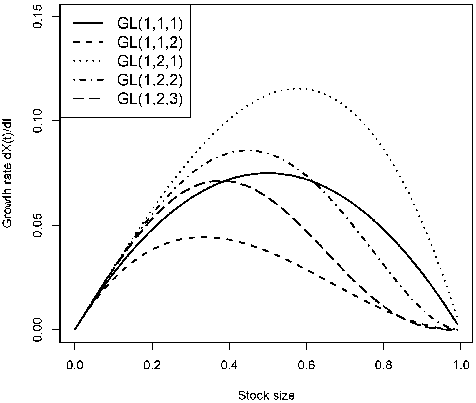
2.1. Generalized Logistic Growth Model

The logistic growth model was introduced by Verhulst [15] in 1838. After that, according to [14], several authors have derived other growth models based on the logistic model. The generalized logistic (GL) growth model considered here can be found in [14] and is provided by the ordinary differential equation (ODE):

$$dX\left(t\right)=r{X}^a\left(t\right){\left(1-{\left(\frac{X\left(t\right)}{K}\right)}^b\right)}^{c}dt,$$

(1)

with positive parameters $a,b$ and c. While negative parameter values can be considered, the risk of losing biological meaning is high. The GL model retains the logistic model’s most important properties, namely, the existence of a horizontal asymptote at $X=K$, the possibility of reaching a maximum value, and the presence of an inflection point. Several other properties and features can be found in [14]. In Equation (1), $X\left(t\right)$ represents the stock size at time instant t, r is the population intrinsic growth rate, and K stands for the carrying capacity (sometimes known as the saturation level).

In the presence of harvesting and under a stochastic environment, the stock dynamic can be modeled by the SDE:

$$dX\left(t\right)=r{X}^a\left(t\right){\left(1-{\left(\frac{X\left(t\right)}{K}\right)}^b\right)}^{c}dt-qE\left(t\right)X\left(t\right)dt+\sigma X\left(t\right)dW\left(t\right),X\left(0\right)=x,$$

(2)

where $X\left(t\right),r$ and K are defined above, $q>0$ is the catchability coefficient, $E\left(t\right)\ge 0$ is the harvesting effort (a Markov control), $\sigma >0$ measures the strength of environmental fluctuations, $W\left(t\right)$ is a standard Wiener process (see for instance [16]), and $x>0$ represents the stock size at the initial time 0. Equation (2) is an Itô autonomous SDE and its solution, $X\left(t\right)$, is a homogeneous diffusion process with drift coefficient $r{X}^a{\left(1-{\left(\frac{X}{K}\right)}^b\right)}^c-qEX$ and diffusion coefficient ${\sigma }^2{X}^2$. In [16,17], after a few adaptations, it is possible to find conditions that allow for a unique solution to Equation (2), provided that the drift and $\sigma X\left(t\right)$ satisfy certain regularity and growth conditions. Hence, it is sufficient to have $0\le E<\frac{r}{q}\left(1-\frac{{\sigma }^2}{2r}\right)$, where $E\left(t\right)\equiv E$ during a small time interval $[t,t+\mathsf{\Delta }t]$ (as in Appendix A).

Two quantities of special interest in harvesting are the yield per unit time $Y\left(t\right)=qE\left(t\right)X\left(t\right)$ and the fishing mortality rate, $F\left(t\right)=qE\left(t\right)$.

For a triplet $(a,b,c)$, we denote Equation (2) by $GL(a,b,c)$, i.e., the generalized logistic growth model with parameters $a,b$, and c. For instance, $GL(1,1,1)$ corresponds to the well known logistic model. Figure 1 shows several curves for the stock growth rate $dX\left(t\right)/dt$ as a function of a stock size $X\left(t\right)$ for several particular cases of the GL model (a deterministic case without harvesting). From [14], and after a few simplifications, we can observe the following well known models: the $GL(1,1,1)$ logistic model, $GL(1,1,2)$ Blumberg’s model (particular case), the $GL(1,2,1)$ and $GL(1,2,2)$ Richards models, and $GL(1,2,3)$, a particular case of a GL model. Other forms of $GL(a,b,c)$ correspond to models that are not specified here, such as the Generalized von Bertalanffy model ($GL(a,1-a,1)$), the Generalized Gompertz model ($GL(1,b\to 0,c)$), and the Hyperbolic model ($GL(1-1/n,1,1+1/n)$).

Figure 1. Stock growth rate, $dX\left(t\right)/dt$, as a function of stock size, $X\left(t\right)$, for several particular cases of the GL model (deterministic case without harvesting).

2.2. Optimal Policy

A stochastic optimal control problem (SOCP) is the process of determining an optimal policy with variable effort based on profit optimization. The profit net value earned by the harvester per unit time, $\mathsf{\Pi }\left(t\right)$, can be defined as the difference between sales revenues per unit time ($R\left(t\right)=(p_1-p_{2}H\left(t\right))H\left(t\right)(p_1>0,p_2\ge 0)$) and harvesting costs per unit time ($C\left(t\right)=(c_1+c_{2}E\left(t\right))E\left(t\right)(c_1>0,c_2>0)$), i.e.,

$$\mathsf{\Pi }\left(t\right)=R\left(t\right)-C\left(t\right)=(p_{1}qX\left(t\right)-c_1)E\left(t\right)-(p_2{q}^2{X}^2\left(t\right)+c_2)E^2\left(t\right).$$

To derive a well-posed SOCP in a finite time, we assume that harvesting occurs within the time interval $[0,T]$. Future harvester profits are discounted at a rate of $\delta >0$, for example, to accounting for currency depreciation and opportunity costs. The optimal harvesting policy maximizes the expected net present value of the total profit. The maximized value of the expected total discounted profit within the interval $[t,T]$, denoted by $J^{*}(X\left(t\right),t)$, is

$$J^{*}(X\left(t\right),t)=\underset{\begin{array}{c}E\left(\tau \right)\\ t\le \tau \le T\end{array}}{max}{\mathbb{E}}_{t,x}\left[\underset{t}{\overset{T}{\int }}{e}^{-\delta (\tau -t)}\mathsf{\Pi }\left(\tau \right)d\tau \right],$$

for which we use the short notation $\mathbb{E}[\dots |X\left(t\right)=y]={\mathbb{E}}_{t,y}[\dots ]$. Finally, the SOCP consists in obtaining the maximized value for the interval $[0,T]$:

$$J^{*}\equiv J^{*}(x,0)=\underset{\begin{array}{c}E\left(\tau \right)\\ 0\le \tau \le T\end{array}}{max}{\mathbb{E}}_{0,x}\left[\underset{0}{\overset{T}{\int }}{e}^{-\delta \tau }\mathsf{\Pi }\left(\tau \right)d\tau \right],$$

(3)

considering $E\left(t\right)$ as a control subject to the population dynamics provided in Equation (2), the control restrictions $0\le E_{min}\le E\left(t\right)\le E_{max}<\infty$, and the terminal condition $J\left(X\right(T),T)=0$.

To obtain the maximized Hamilton–Jacobi–Bellman (HJB) equation, the following SOCP is solved using stochastic dynamic programming (see pp. 259–268 in [18] along with [19,20]), as detailed in Appendix A:

$$\begin{array}{cc}\hfill -\frac{\partial J^{*}(X\left(t\right),t)}{\partial t}=& \left(p_{1}qX\left(t\right)-c_1-(p_2{q}^2{X}^2\left(t\right)+c_2)E^{*}\left(t\right)\right)E^{*}\left(t\right)-\delta J^{*}(X\left(t\right),t)\hfill \\ & +\frac{\partial J^{*}(X\left(t\right),t)}{\partial X\left(t\right)}\left(r{X}^a\left(t\right){\left(1-{\left(\frac{X\left(t\right)}{K}\right)}^b\right)}^c-q{E}^{*}\left(t\right)X\left(t\right)\right)\hfill \\ & +\frac{1}{2}\frac{{\partial }^2{J}^{*}(X\left(t\right),t)}{\partial X^2\left(t\right)}{\sigma }^2{X}^2\left(t\right),\hfill \end{array}$$

(4)

which represents the expected total discounted profit. The optimal variable effort is

$$E^{*}\left(t\right)=\left\{\begin{array}{cc}{E}_{min},\hfill & \mathrm{if}{E}_u^{*}\left(t\right)<E_{min}\hfill \\ E_u^{*}\left(t\right),\hfill & \mathrm{if}{E}_{min}\le E_u^{*}\left(t\right)\le E_{max}\hfill \\ E_{max},\hfill & \mathrm{if}{E}_u^{*}\left(t\right)>E_{max},\hfill \end{array}\right.$$

where

$$E_u^{*}\left(t\right)={\displaystyle \frac{\left(p_1-\frac{\partial J^{*}(X\left(t\right),t)}{\partial X\left(t\right)}\right)qX\left(t\right)-c_1}{2\left(p_2{q}^{2}X{\left(t\right)}^2+c_2\right)}}$$

(5)

is the unconstrained effort (as in [21]), which can be denoted by the optimal variable effort as well.

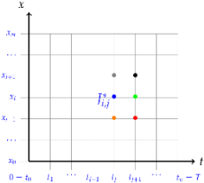
2.3. Domain Discretization and Finite Difference Approximation

The HJB Equation (4) is a nonlinear parabolic PDE involving a temporal variable and a spatial variable. Unfortunately, it is impossible to solve it analytically, and thusu we resort to numerical methods and apply a Crank–Nicolson discretization scheme based on finite differences. This problem’s natural domain is $[0,T]\times \mathbf{R}$; however, to obtain a numerical solution it is necessary to define a bounded computational domain. As a result, we define the bounded domain as $[0,T]\times [0,x_{max}]$ with $x_{max}$ such that the probability of $X\left(t\right)$ exceeding $x_{max}$ is negligible. Moreover, we consider uniform grids in space and time domains as follows:

The partitions for space and time are

$$x_i=x_0+i\mathsf{\Delta }x,i=1,\dots ,m,\mathsf{\Delta }x=x_{max}/m,$$

$$t_j=t_0+j\mathsf{\Delta }t,j=1,\dots ,n,\mathsf{\Delta }t=T/n.$$

They form a grid of points where $J_{i,j}^{*}:=J^{*}(x_i,t_j)$ and $E_{i,j}^{*}:=E^{*}(x_i,t_j)$, with $0\le i\le m$ and $0\le j\le n$. Because the boundary condition $J^{*}(X\left(T\right),T)=0$ is terminal rather than initial, the computation uses time to move backwards from T to 0.

As in [22], the space derivatives are approximated by central differences obtained by averaging the regressive and progressive approximations (for $0\le j\le n-1$):

$$\begin{array}{ccc}\hfill \frac{\partial J_{i,j}^{*}}{\partial x}& \approx & \frac{1}{2}\left(\frac{J_{i+1,j+1}^{*}-J_{i-1,j+1}^{*}}{2\mathsf{\Delta }x}+\frac{J_{i+1,j}^{*}-J_{i-1,j}^{*}}{2\mathsf{\Delta }x}\right),1\le i\le m-1,\hfill \\ \hfill \frac{{\partial }^2{J}_{i,j}^{*}}{\partial x^2}& \approx & \frac{1}{2}\left(\frac{J_{i+1,j+1}^{*}-2J_{i,j+1}^{*}+J_{i-1,j+1}^{*}}{\mathsf{\Delta }{x}^2}+\frac{J_{i+1,j}^{*}-2J_{i,j}^{*}+J_{i-1,j}^{*}}{\mathsf{\Delta }{x}^2}\right),1\le i\le m-1,\hfill \\ \hfill \frac{\partial J_{m,j}^{*}}{\partial x}& \approx & \frac{1}{2}\left(\frac{3J_{m,j+1}^{*}-4J_{m-1,j+1}^{*}+J_{m-2,j+1}^{*}}{2\mathsf{\Delta }x}+\frac{3J_{m,j}^{*}-4J_{m-1,j}^{*}+J_{m-2,j}^{*}}{2\mathsf{\Delta }x}\right),i=m,\hfill \end{array}$$

and

$$\begin{array}{cc}\hfill \frac{{\partial }^2{J}_{m,j}^{*}}{\partial x^2}\approx & \frac{1}{2}\left(\frac{3J_{m,j+1}^{*}-7J_{m-1,j+1}^{*}+5J_{m-2,j+1}^{*}-J_{m-3,j+1}^{*}}{\mathsf{\Delta }{x}^2}\right)\hfill \\ & +\frac{1}{2}\left(\frac{3J_{m,j}^{*}-7J_{m-1,j}^{*}+5J_{m-2,j}^{*}-J_{m-3,j}^{*}}{\mathsf{\Delta }{x}^2}\right),i=m.\hfill \end{array}$$

(6)

The time derivative is approximated using a two time instant scheme:

$$\frac{\partial J_{i,j}^{*}}{\partial t}\approx \frac{J_{i,j+1}^{*}-J_{i,j}^{*}}{\mathsf{\Delta }t},0\le i\le m,0\le j\le n-1.$$

2.4. Numerical Solution

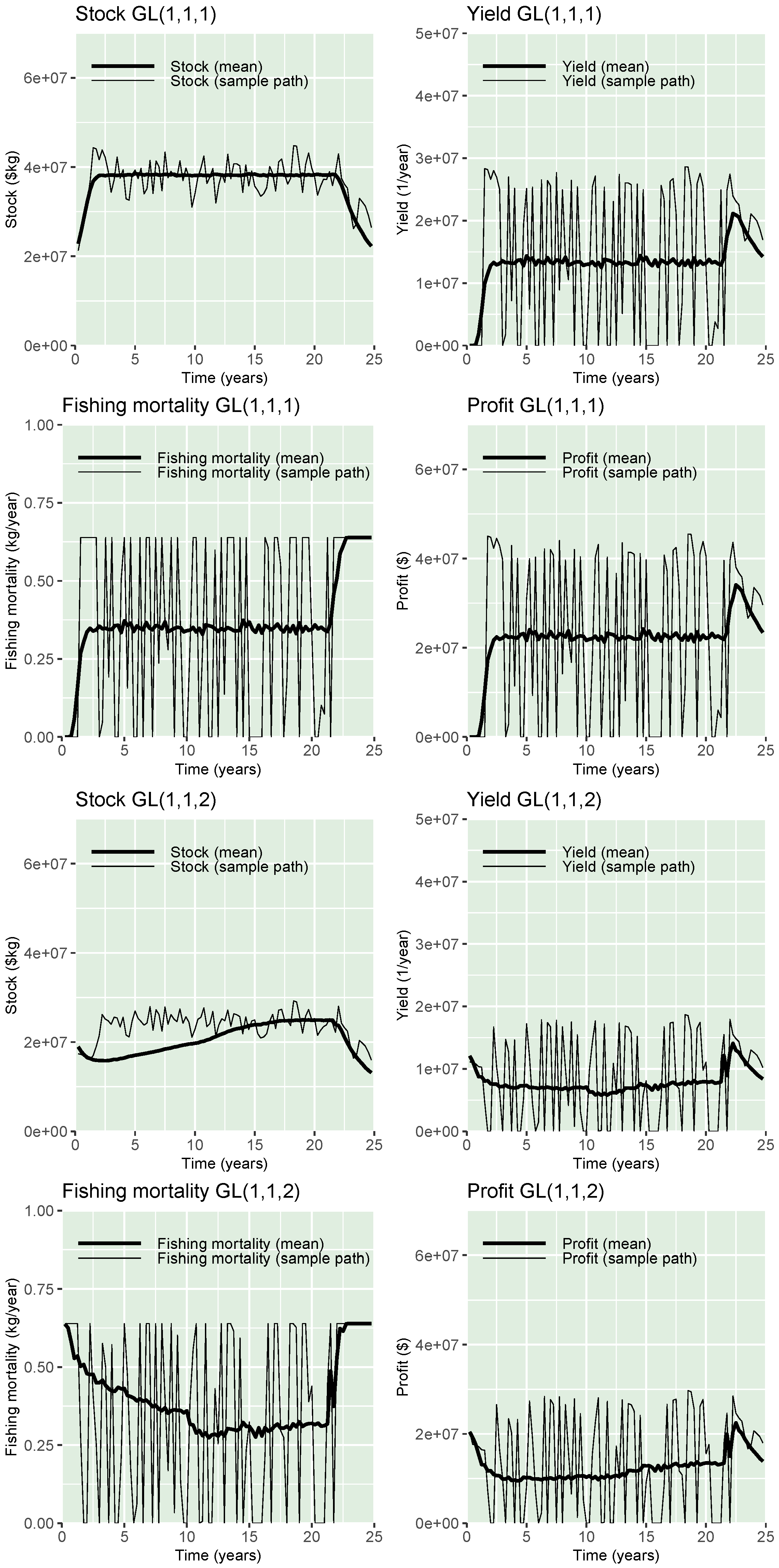
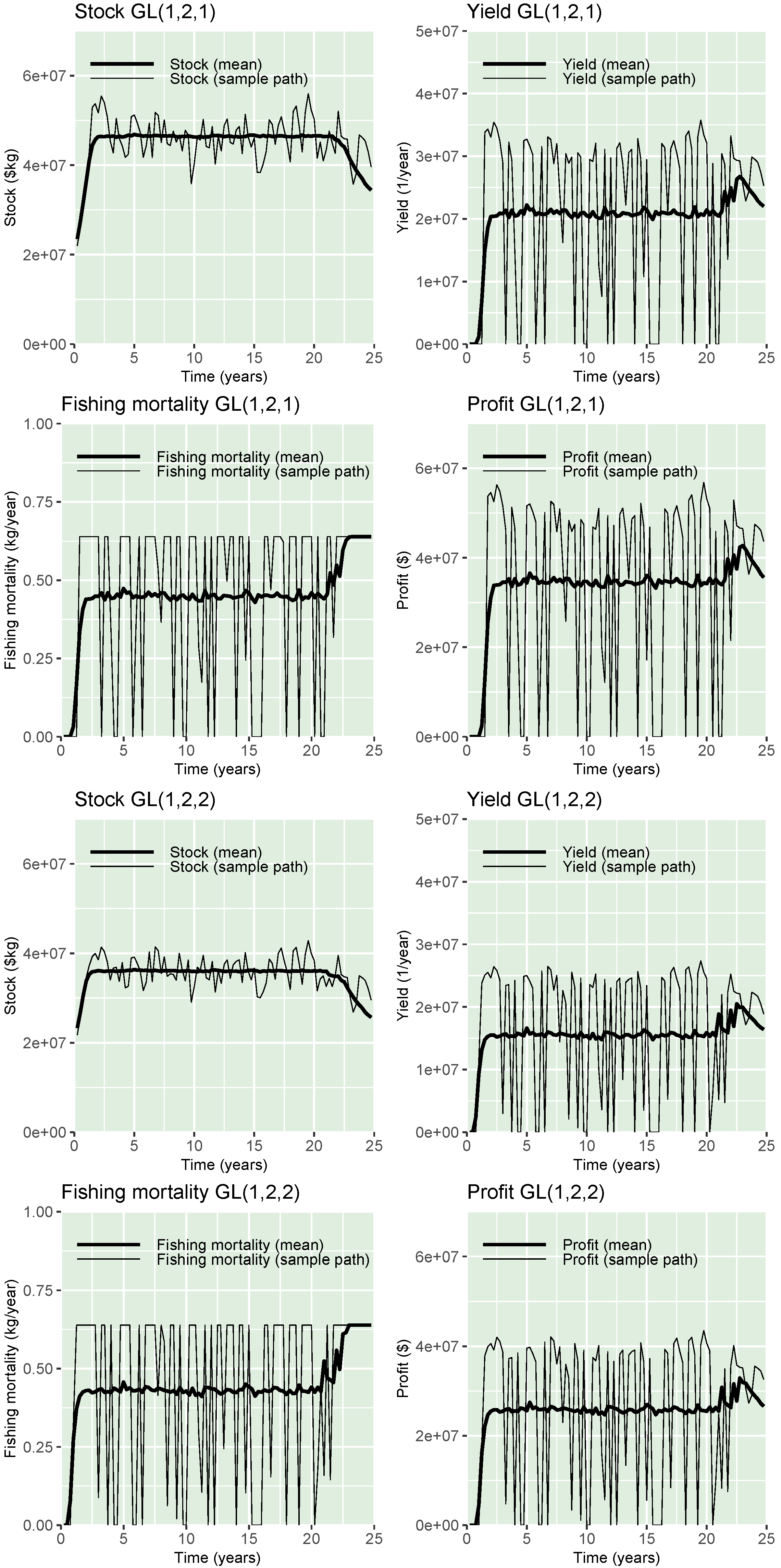
Using the above approximations, the discretized version of the HJB Equation (4) is (for $0\le j\le n-1$)

$$\begin{array}{ccc}\hfill -\frac{J_{i,j+1}^{*}-J_{i,j}^{*}}{\mathsf{\Delta }t}& =& (p_{1}q{x}_i-c_1)E_{i,j+1}^{*}-(p_2{q}^2{x}_i^2+c_2)E_{i,j+1}^{*2}-\delta \left(\frac{J_{i,j+1}^{*}}{2}+\frac{J_{i,j}^{*}}{2}\right)\hfill \\ & +& \frac{1}{2}\left(\frac{J_{i+1,j+1}^{*}-J_{i-1,j+1}^{*}}{2\mathsf{\Delta }x}+\frac{J_{i+1,j}^{*}-J_{i-1,j}^{*}}{2\mathsf{\Delta }x}\right)\left(f\left(x_i\right)-q{E}_{i,j+1}^{*}\right)x_i\hfill \\ & +& \frac{1}{4}\left(\frac{J_{i+1,j+1}^{*}-2J_{i,j+1}^{*}+J_{i-1,j+1}^{*}}{\mathsf{\Delta }{x}^2}+\frac{J_{i+1,j}^{*}-2J_{i,j}^{*}+J_{i-1,j}^{*}}{\mathsf{\Delta }{x}^2}\right){\sigma }^2{x}_i^2,\hfill \\ \hfill \mathrm{for} 1\le i\le m-1,\end{array}$$

and

$$\begin{array}{ccc}\hfill -\frac{J_{m,j+1}^{*}-J_{m,j}^{*}}{\mathsf{\Delta }t}& =& (p_{1}q{x}_m-c_1)E_{m,j+1}^{*}-(p_2{q}^2{x}_m^2+c_2)E_{m,j+1}^{*2}-\delta \left(\frac{J_{m,j+1}^{*}}{2}+\frac{J_{m,j}^{*}}{2}\right)\hfill \\ & +& \frac{1}{2}\left(\frac{3J_{m,j+1}^{*}-4J_{m-1,j+1}^{*}+J_{m-2,j+1}^{*}}{2\mathsf{\Delta }x}+\frac{3J_{m,j}^{*}-4J_{m-1,j}^{*}+J_{m-2,j}^{*}}{2\mathsf{\Delta }x}\right)\hfill \\ & \times & \left(f\left(x_m\right)-q{E}_{m,j+1}^{*}\right)x_m+\frac{1}{4}(\frac{3J_{m,j+1}^{*}-7J_{m-1,j+1}^{*}+5J_{m-2,j+1}^{*}-J_{m-3,j+1}^{*}}{\mathsf{\Delta }{x}^2}\hfill \\ & +& \frac{3J_{m,j}^{*}-7J_{m-1,j}^{*}+5J_{m-2,j}^{*}-J_{m-3,j}^{*}}{\mathsf{\Delta }{x}^2}){\sigma }^2{x}_m^2,i=m,\hfill \end{array}$$

with $f\left(x_i\right)=r{x}_i^{a-1}{\left(1-{\left(\frac{x_i}{K}\right)}^b\right)}^c,i=1,\dots ,m$ in both expressions.

The discretized version of the unconstrained optimal effort (5) is

$$E_{u,i,j}^{*}={\displaystyle \frac{\left(p_1-\frac{\partial J_{i,j}^{*}}{\partial x}\right)q{x}_i-c_1}{2\left(p_2{q}^2{x}_i^2+c_2\right)}}={\displaystyle \frac{\left(p_1-\frac{1}{2}\left(\frac{J_{i+1,j+1}^{*}-J_{i-1,j+1}^{*}}{2\mathsf{\Delta }x}+\frac{J_{i+1,j}^{*}-J_{i-1,j}^{*}}{2\mathsf{\Delta }x}\right)\right)q{x}_i-c_1}{2\left(p_2{q}^2{x}_i^2+c_2\right)}},$$

for $1\le i\le m-1$, and

$$\begin{array}{cc}\hfill E_{u,m,j}^{*}=& {\displaystyle \frac{\left(p_1-\frac{\partial J_{m,j}^{*}}{\partial x}\right)q{x}_m-c_1}{2\left(p_2{q}^2{x}_m^2+c_2\right)}}\hfill \\ & ={\displaystyle \frac{\left(p_1-\frac{1}{2}\left(\frac{3J_{m,j+1}^{*}-4J_{m-1,j+1}^{*}+J_{m-2,j+1}^{*}}{2\mathsf{\Delta }x}+\frac{3J_{m,j}^{*}-4J_{m-1,j}^{*}+J_{m-2,j}^{*}}{2\mathsf{\Delta }x}\right)\right)q{x}_m-c_1}{2\left(p_2{q}^2{x}_m^2+c_2\right)}},\hfill \end{array}$$

(7)

for $i=m$.

The discretized version of the HJB equation can be written as a system of m equations (for $0\le j\le n-1$)

$$\begin{array}{c}\hfill \left(\frac{(f\left(x_i\right)-q{E}_{i,j+1}^{*})x_i\mathsf{\Delta }t}{4\mathsf{\Delta }x}-\frac{{\sigma }^2{x}_i^2\mathsf{\Delta }t}{4\mathsf{\Delta }{x}^2}\right){\mathit{J}}_{\mathit{i}-\mathbf{1},\mathit{j}}^{\mathbf{*}}+\left(1+\frac{\delta \mathsf{\Delta }t}{2}+\frac{{\sigma }^2{x}_i^2\mathsf{\Delta }t}{2\mathsf{\Delta }{x}^2}\right){\mathit{J}}_{\mathit{i},\mathit{j}}^{\mathbf{*}}\\ \hfill -\left(\frac{(f\left(x_i\right)-q{E}_{i,j+1}^{*})x_i\mathsf{\Delta }t}{4\mathsf{\Delta }x}+\frac{{\sigma }^2{x}_i^2\mathsf{\Delta }t}{4\mathsf{\Delta }{x}^2}\right){\mathit{J}}_{\mathit{i}+\mathbf{1},\mathit{j}}^{\mathbf{*}}\\ \hfill =\\ \hfill \left(\frac{-(f\left(x_i\right)-q{E}_{i,j+1}^{*})x_i\mathsf{\Delta }t}{4\mathsf{\Delta }x}+\frac{{\sigma }^2{x}_i^2\mathsf{\Delta }t}{4\mathsf{\Delta }{x}^2}\right){\mathit{J}}_{\mathit{i}-\mathbf{1},\mathit{j}+\mathbf{1}}^{\mathbf{*}}+\left(1-\frac{\delta \mathsf{\Delta }t}{2}-\frac{{\sigma }^2{x}_i^2\mathsf{\Delta }t}{2\mathsf{\Delta }{x}^2}\right)·{\mathit{J}}_{\mathit{i},\mathit{j}+\mathbf{1}}^{\mathbf{*}}\\ \hfill +\left(\frac{(f\left(x_i\right)-q{E}_{i,j+1}^{*})x_i\mathsf{\Delta }t}{4\mathsf{\Delta }x}+\frac{{\sigma }^2{x}_i^2\mathsf{\Delta }t}{4\mathsf{\Delta }{x}^2}\right){\mathit{J}}_{\mathit{i}+\mathbf{1},\mathit{j}+\mathbf{1}}^{\mathbf{*}}\\ \hfill +(p_{1}q{x}_i-c_1)E_{i,j+1}^{*}\mathsf{\Delta }t-(p_2{q}^2{x}_i^2+c_2)E_{i,j+1}^{*2}\mathsf{\Delta }t,1\le i\le m-1,\end{array}$$

and

$$\begin{array}{c}\hfill \frac{{\sigma }^2{x}_m^2\mathsf{\Delta }t}{4\mathsf{\Delta }{x}^2}·{\mathit{J}}_{\mathit{m}-\mathbf{3},\mathit{j}}^{\mathbf{*}}-\left(\frac{(f\left(x_m\right)-q{E}_{m,j+1}^{*})x_m\mathsf{\Delta }t}{4\mathsf{\Delta }x}+\frac{5{\sigma }^2{x}_m^2\mathsf{\Delta }t}{4\mathsf{\Delta }{x}^2}\right)·{\mathit{J}}_{\mathit{m}-\mathbf{2},\mathit{j}}^{\mathbf{*}}\\ \hfill +\left(\frac{(f\left(x_m\right)-q{E}_{m,j+1}^{*})x_m\mathsf{\Delta }t}{\mathsf{\Delta }x}+\frac{7{\sigma }^2{x}_m^2\mathsf{\Delta }t}{4\mathsf{\Delta }{x}^2}\right)·{\mathit{J}}_{\mathit{m}-\mathbf{1},\mathit{j}}^{\mathbf{*}}\\ \hfill +\left(1+\frac{\delta \mathsf{\Delta }t}{2}-\frac{3(f\left(x_m\right)-q{E}_{m,j+1}^{*})x_m\mathsf{\Delta }t}{4\mathsf{\Delta }x}-\frac{3{\sigma }^2{x}_m^2\mathsf{\Delta }t}{4\mathsf{\Delta }{x}^2}\right)·{\mathit{J}}_{\mathit{m},\mathit{j}}^{\mathbf{*}}\\ \hfill =-\frac{{\sigma }^2{x}_m^2\mathsf{\Delta }t}{4\mathsf{\Delta }{x}^2}·{\mathit{J}}_{\mathit{m}-\mathbf{3},\mathit{j}+\mathbf{1}}^{\mathbf{*}}+\left(\frac{(f\left(x_m\right)-q{E}_{m,j+1}^{*})x_m\mathsf{\Delta }t}{4\mathsf{\Delta }x}+\frac{5{\sigma }^2{x}_m^2\mathsf{\Delta }t}{4\mathsf{\Delta }{x}^2}\right)·{\mathit{J}}_{\mathit{m}-\mathbf{2},\mathit{j}+\mathbf{1}}^{\mathbf{*}}\\ \hfill -\left(\frac{(f\left(x_m\right)-q{E}_{m,j+1}^{*})x_m\mathsf{\Delta }t}{\mathsf{\Delta }x}+\frac{7{\sigma }^2{x}_m^2\mathsf{\Delta }t}{4\mathsf{\Delta }{x}^2}\right)·{\mathit{J}}_{\mathit{m}-\mathbf{1},\mathit{j}+\mathbf{1}}^{\mathbf{*}}\\ \hfill +\left(1-\frac{\delta \mathsf{\Delta }t}{2}+\frac{3(f\left(x_m\right)-q{E}_{m,j+1}^{*})x_m\mathsf{\Delta }t}{4\mathsf{\Delta }x}+\frac{3{\sigma }^2{x}_m^2\mathsf{\Delta }t}{4\mathsf{\Delta }{x}^2}\right)·{\mathit{J}}_{\mathit{m},\mathit{j}+\mathbf{1}}^{\mathbf{*}}\\ \hfill +(p_{1}q{x}_m-c_1)E_{m,j+1}^{*}\mathsf{\Delta }t-(p_2{q}^2{x}_m^2+c_2)E_{m,j+1}^{*2}\mathsf{\Delta }t,i=m.\end{array}$$

The system can be written using the appropriate matrices A, B, and C in the form

$$A{\mathit{J}}_{-}^{\mathbf{*}}=B{\mathit{J}}_{+}^{\mathbf{*}}+C,$$

with

$${\mathit{J}}_{-}^{\mathbf{*}}=\left[\begin{array}{ccccccc}{\mathit{J}}_{\mathbf{0}}^{\mathbf{*}}& |& {\mathit{J}}_{\mathbf{1}}^{\mathbf{*}}& |& \cdots & |& {\mathit{J}}_{\mathit{n}-\mathbf{1}}^{\mathbf{*}}\end{array}\right],{\mathit{J}}_{+}^{*}=\left[\begin{array}{ccccccc}{\mathit{J}}_{\mathbf{1}}^{\mathbf{*}}& |& {\mathit{J}}_{\mathbf{2}}^{\mathbf{*}}& |& \cdots & |& {\mathit{J}}_{\mathit{n}}^{\mathbf{*}}\end{array}\right],\mathrm{and}$$

$${\mathit{J}}_{\mathit{j}}^{\mathbf{*}}={\left[\begin{array}{ccccc}{J}_{0,j}^{*}& & J_{1,j}^{*}& \cdots & J_{m,j}^{*}\end{array}\right]}^T,0\le j\le n,$$

where T is the transpose operator. Solving the system, we obtain the optimal solution for the grid points. Polynomial interpolation between the values at the neighbouring points of X in the partition $x_0,x_1,\dots ,x_m$ yields the optimal solution when the stock is at a given value X at a time $t_k$.

3. Results

To compute $J^{*}$, that is, the profit earned by the harvester during the interval $[0,T]$, we performed 1000 Monte Carlo simulations for the stock, the effort, and the profit. The stock dynamics were simulated based on a Euler scheme. In [2,21], we discovered a fairly complete set of parameter values (namely, $r,K,q,p_1,p_2,c_1$, and $c_2$) for the Pacific halibut (Hippoglossus hippoglossus). The other parameters ($E_{min},E_{max},\sigma ,x,\delta ,n,m$ and $x_{max}$), for which we had no data, were empirically chosen to be reasonable, and the time horizon was set at $T=25$ years. It is important to keep in mind that n and m were chosen from a pool of several trials in order for the algorithm to reach convergence. We were unable to estimate any parameters due to the lack of historical data, namely, stock size and harvesting effort. Table 1 contains the complete set of parameter values.

Table 1. Parameter values used to run the simulations. The definition of an SFU (Standardized Fishing Unit) is explained in [21].

Parameter	Description	Value	Unit
r	Intrinsic growth rate	$0.71$	${\mathrm{y}\mathrm{e}\mathrm{a}\mathrm{r}}^{-1}$
K	Carrying capacity	$80.5\times {10}^6$	kg
q	Catchability coefficient	$3.30\times {10}^{-6}$	${\mathrm{S}\mathrm{F}\mathrm{U}}^{-1}{\mathrm{y}\mathrm{e}\mathrm{a}\mathrm{r}}^{-1}$
$E_{min}$	Minimum fishing effort	0	SFU
$E_{max}$	Maximum fishing effort	$0.9 r/q$	SFU
$\sigma$	Strength of environmental fluctuations	$0.15$	${\mathrm{y}\mathrm{e}\mathrm{a}\mathrm{r}}^{-1/2}$
x	Initial population size	$0.25$K	kg
$\delta$	Discount factor	$0.03$	${\mathrm{y}\mathrm{e}\mathrm{a}\mathrm{r}}^{-1}$
$p_1$	Linear price coefficient	$1.59$	$\${\mathrm{k}\mathrm{g}}^{-1}$
$p_2$	Quadratic price coefficient	0	$\$\mathrm{y}\mathrm{e}\mathrm{a}\mathrm{r}\times {\mathrm{k}\mathrm{g}}^{-2}$
$c_1$	Linear cost coefficient	$96\times {10}^{-6}$	$\${\mathrm{S}\mathrm{F}\mathrm{U}}^{-1}{\mathrm{y}\mathrm{e}\mathrm{a}\mathrm{r}}^{-1}$
$c_2$	Quadratic cost coefficient	${10}^{-7}$	$\${\mathrm{S}\mathrm{F}\mathrm{U}}^{-2}{\mathrm{y}\mathrm{e}\mathrm{a}\mathrm{r}}^{-1}$
T	Time horizon	25	year
n	Number of time sub-intervals	100
$x_{max}$	Maximum stock size	$2K$	kg
m	Number of sub-intervals for the space state (b)	100

The models chosen to obtain the optimal policies were the ones referenced before as particular cases of the GL growth model in Section 2.1. For each one, we ran 1000 simulations to obtain the optimal effort and optimal profit. The results are listed in Table 2.

Table 2. Optimal profit and standard deviation values for the particular cases of the GL growth model in Section 2.1. Values are in millions of US dollars. SD represents standard deviation.

Model Representation	J*	SD
$GL(1,1,1)$	374.148	32.351
$GL(1,1,2)$	214.864	32.205
$GL(1,2,1)$	565.456	38.365
$GL(1,2,2)$	432.174	30.185
$GL(1,2,3)$	366.377	25.182

It can be observed from Table 2 that the highest profit, USD $565.456M$, comes from the application of model $GL(1,2,1)$, followed by models $GL(1,2,2)$, $GL(1,1,1)$, $GL(1,2,3)$, and $GL(1,1,2)$, in decreasing order. This is not a surprise, as $GL(1,2,1)$ is, according to Figure 1, the one with a higher growth rate. Model $GL(1,1,2)$ yields the lowest profit value, USD $214.864M$, and is the model with the lowest growth rate, as seen in Figure 1. In terms of standard deviation, the highest value is related to model $GL(1,2,1)$ and the lowest is related to model $GL(1,2,3)$. The remaining models have identical values.

For the models presented in Table 2, Figure 2, Figure 3 and Figure 4 depict what could happen when applying the optimal harvesting policy to such growth models. The thin lines represent one possible reality in each image that a harvester would experience (one of the 1000 simulations). The thicker lines represent the mean of 1000 simulations, which is a good approximation of the expected value appearing in the expression (3). For each model, a trajectory and sample mean for the stock size $X\left(t\right)$, yield $Y\left(t\right)=qE\left(t\right)X\left(t\right)$, fishing mortality $F\left(t\right)=qE\left(t\right)$, and optimal profit per unit time can be found. Conclusions based on Figure 2, Figure 3 and Figure 4 are similar to the results presented in Table 2. Indeed, model $GL(1,2,1)$ shows the largest stock size compared with other models, implying higher fishing mortality.

Figure 2. Stock, fishing mortality, yield, and profit sample paths (thinner line) and mean (ticker line) obtained by the application of models $GL(1,1,1)$ (top panel) and $GL(1,1,2)$ (bottom panel). Unit values are described in Table 1.

Figure 3. Stock, fishing mortality, yield, and profit sample paths (thinner line) and mean (ticker line) obtained by the application of models $GL(1,2,1)$ (top panel) and $GL(1,2,2)$ (bottom panel). Unit values are described in Table 1.

Figure 4. Stock, fishing mortality, yield, and profit sample paths (thinner line) and mean (ticker line) obtained by the application of model $GL(1,2,3)$. Unit values are described in Table 1.

Sensitivity Analysis

We now examine the implications of changing the values of $\delta$, $c_1$, $c_2$, and $\sigma$ from the ones in Table 2 used for the simulations. To perform a sensitivity analysis, we chose the $GL(1,2,3)$ model and ran simulations identical the the ones before while changing each parameter one at a time. A summary of the alternative parameter values and the obtained profit per unit time is provided in Table 3.

Table 3. Alternative parameter values for model $GL(1,2,3)$. The parameters used to perform the sensitivity analysis were $\delta ,c_1,c_2$ and $\sigma$. Profit and standard deviation values are in millions of US dollars. SD represents standard deviation.

Parameter	Value	J*	SD	Parameter	Value	J*	SD
$\delta$	$0.03$	366.377	25.182	$c_2$	${10}^{-7}$	366.377	25.182
	$0.10$	183.553	14.512		${10}^{-5}$	362.629	25.107
	$0.15$	126.953	11.153		${10}^{-3}$	187.007	13.932
$c_1$	$96\times {10}^{-6}$	366.377	25.182	$\sigma$	$0.15$	366.377	25.182
	$96\times {10}^{-4}$	366.355	25.181		$0.30$	354.345	49.656
	$96\times {10}^{-2}$	364.146	25.048		$0.45$	270.540	81.259

Increasing the value of $\delta$ has a large effect on the profit value and implies a decrease of about $50\%$. This is to be expected, as the increase in $\delta$ represents a depreciation in the value of the currency. A greater depreciation ($\delta =0.15$) implies a greater loss of profit. The initial value of $c_1$ is shallow, and thus the increase to $96\times {10}^{-4}$ is negligible. However, increasing that value to $96\times {10}^{-2}$ reduces the profit, as expected. An increase in $c_2$ has implications for profit reduction, and may imply a $50\%$ profit reduction. We note that $c_2$ represents unexpected costs (unspecialized gear and/or vessels) typically associated with extra costs. The influence of stochastic fluctuations is analysed by changing values of $\sigma$. A rise in stochastic fluctuations, i.e., $\sigma =0.30$ or $\sigma =0.45$, has a huge influence on profit. The values of the standard deviation show such implications.

4. Conclusions

In this paper, we have worked with a stochastic differential equation generalized logistic stock growth model. From this model, we show how to obtain particular models typically used for harvesting problems. We have formulated a stochastic optimal control problem to obtain the optimal variable effort policy. We deduced the HJB equation using dynamic programming techniques and showed its solution through numerical methods by applying a Crank–Nicolson discretization scheme. We have applied the optimal policy for several particular models, considering realistic parameter values estimated from real stock. We conclude that models with a higher growth rate imply higher profit values, as expected. In addition, we examined the sensitivity of the expected total discounted profit to the discount factor, cost parameters, and stochastic environmental fluctuations.

References

- Beddington, J.R.; May, R.M. Harvesting natural populations in a randomly fluctuating environment. Science 1977, 197, 463–465. [Google Scholar] [CrossRef] [PubMed]
- Clark, C.W. Mathematical Bioeconomics: The Optimal Management of Renewable Resources, 2nd ed.; Wiley: New York, NY, USA, 1990. [Google Scholar]
- Alvarez, L.H.R.; Sheep, L.A. Optimal harvesting of stochastically fluctuating populations. J. Math. Biol. 1998, 37, 155–177. [Google Scholar] [CrossRef]
- Alvarez, L.H.R. On the option interpretation of rational harvesting planning. J. Math. Biol. 2000, 40, 383–405. [Google Scholar] [CrossRef]
- Alvarez, L.H.R. Singular stochastic control in the presence of a state-dependent yield structure. Stoch. Process. Their Appl. 2000, 86, 323–343. [Google Scholar] [CrossRef]
- Brites, N.M.; Braumann, C.A. Harvesting in a Random Varying Environment: Optimal, Stepwise and Sustainable Policies for the Gompertz Model. Stat. Optim. Inf. Comput. 2019, 7, 533–544. [Google Scholar] [CrossRef]
- Brites, N.M.; Braumann, C.A. Harvesting optimization with stochastic differential equations models: Is the optimal enemy of the good? Stoch. Model. 2021, 0, 1–19. [Google Scholar] [CrossRef]
- Brites, N.M.; Braumann, C.A. Profit optimization of stochastically fluctuating populations: The effects of Allee effects. Optimization 2022, 1–12. [Google Scholar] [CrossRef]
- Brites, N.M.; Braumann, C.A. Fisheries management in random environments: Comparison of harvesting policies for the logistic model. Fish. Res. 2017, 195, 238–246. [Google Scholar] [CrossRef]
- Brites, N.M.; Braumann, C.A. Fisheries management in randomly varying environments: Comparison of constant, variable and penalized efforts policies for the Gompertz model. Fish. Res. 2019, 216, 196–203. [Google Scholar] [CrossRef]
- Brites, N.M.; Braumann, C.A. Stochastic differential equations harvesting policies: Allee effects, logistic-like growth and profit optimization. Appl. Stoch. Model. Bus. Ind. 2020, 36, 825–835. [Google Scholar] [CrossRef]
- Brites, N.M.; Braumann, C.A. Harvesting Policies with Stepwise Effort and Logistic Growth in a Random Environment. In Current Trends in Dynamical Systems in Biology and Natural Sciences; Aguiar, M., Braumann, C., Kooi, B.W., Pugliese, A., Stollenwerk, N., Venturino, E., Eds.; Springer: Cham, Switzerland, 2020; pp. 95–110. [Google Scholar] [CrossRef]
- Shah, M.A.; Sharma, U. Optimal harvesting policies for a generalized Gordon–Schaefer model in randomly varying environment. Appl. Stoch. Model. Bus. Ind. 2003, 19, 43–49. [Google Scholar] [CrossRef]
- Tsoularis, A.; Wallace, J. Analysis of logistic growth models. Math. Biosci. 2002, 179, 21–55. [Google Scholar] [CrossRef]
- Verhulst, P.F. Notice sur la loi que la population poursuit dans son accroissement. Corresp. Math. Phys. 1838, 10, 113–121. [Google Scholar]
- Braumann, C.A. Stochastic differential equation models of fisheries in an uncertain world: Extinction probabilities, optimal fishing effort, and parameter estimation. In Proceedings of the Mathematics in Biology and Medicine, Bari, Italy, 18–22 July 1985; Capasso, V., Grosso, E., Paveri-Fontana, S.L., Eds.; Springer: Berlin, Germany, 1985; pp. 201–206. [Google Scholar]
- Braumann, C.A. Introduction to Stochastic Differential Equations with Applications to Modelling in Biology and Finance; John Wiley & Sons, Inc.: New York, NY, USA, 2019. [Google Scholar]
- Kamien, M.I.; Schwartz, N.L. Dynamic Optimization; North-Holland, The Netherlands, 1993. [Google Scholar]
- Fleming, W.H.; Soner, H.M. Controlled Markov Processes and Viscosity Solutions; Springer: New York, NY, USA, 2006. [Google Scholar]
- Touzi, N. Optimal Stochastic Control, Stochastic Target Problems, and Backward SDE; Springer: New York, NY, USA, 2013. [Google Scholar]
- Hanson, F.B.; Ryan, D. Optimal harvesting with both population and price dynamics. Math. Biosci. 1998, 148, 129–146. [Google Scholar] [CrossRef]
- LeVeque, R.J. Finite Difference Methods for Ordinary and Partial Differential Equations; Society for Industrial and Applied Mathematics: Philadelphia, PA, USA, 2007. [Google Scholar] [CrossRef]
Publisher’s Note: MDPI stays neutral with regard to jurisdictional claims in published maps and institutional affiliations. |
© 2022 by the author. Licensee MDPI, Basel, Switzerland. This article is an open access article distributed under the terms and conditions of the Creative Commons Attribution (CC BY) license (https://creativecommons.org/licenses/by/4.0/).