
Numerical Analyses and a Nonlinear Composite Controller for a Real-Time Ground Aerodynamic Heating Simulation of a Hypersonic Flying Object

 ,
,
Abstract
:1. Introduction
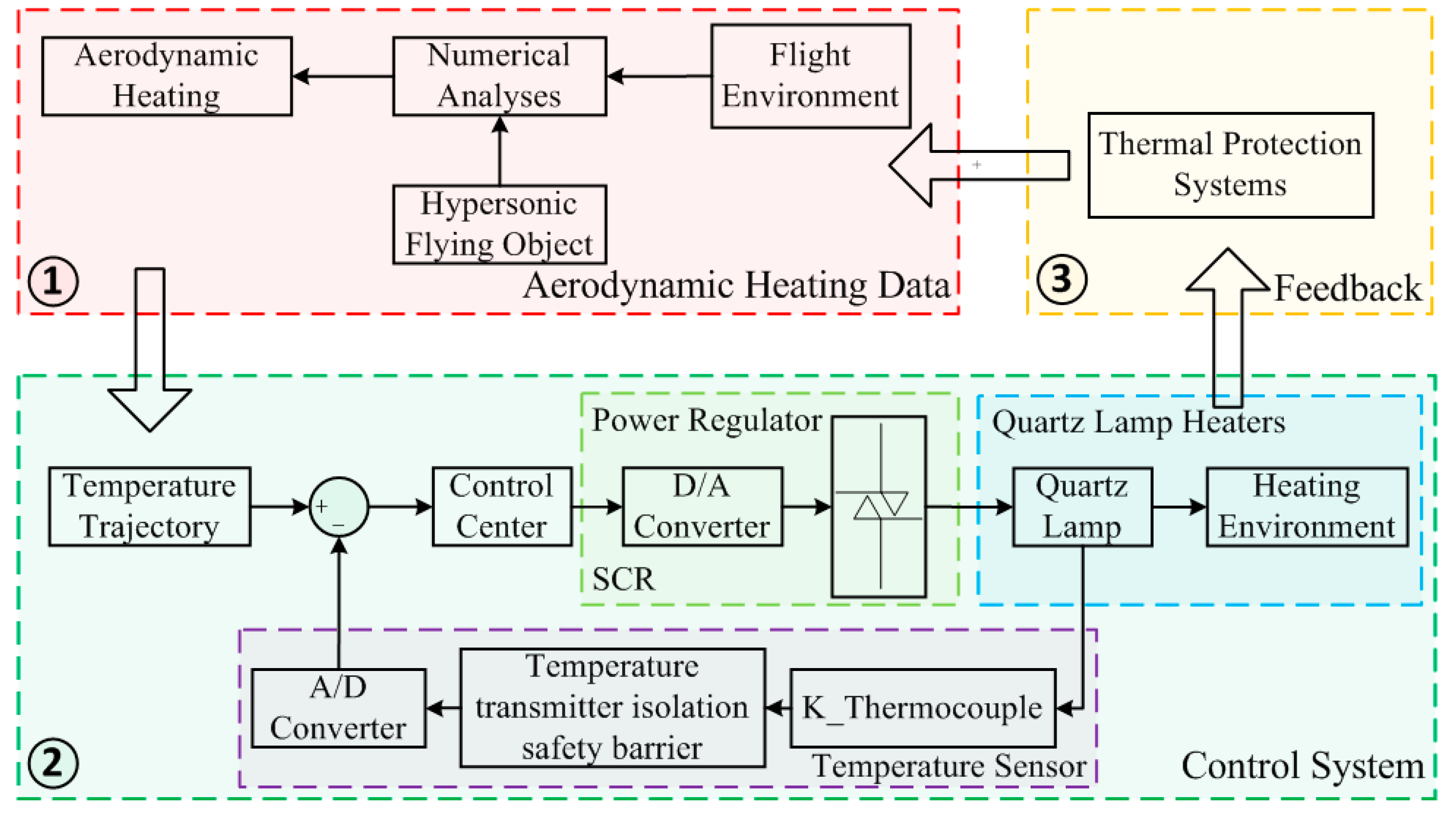
- Numerical analyses of a hypersonic flying object’s aerodynamic heating environment are based on three different two-dimensional outflow fields via finite element calculation in ANSYS Workbench 2020 R2.
- The composite controller control strategy is proposed for the TSTQLs, which can provide a model free frame being independent of the system dynamic model along with an ultra-local model.
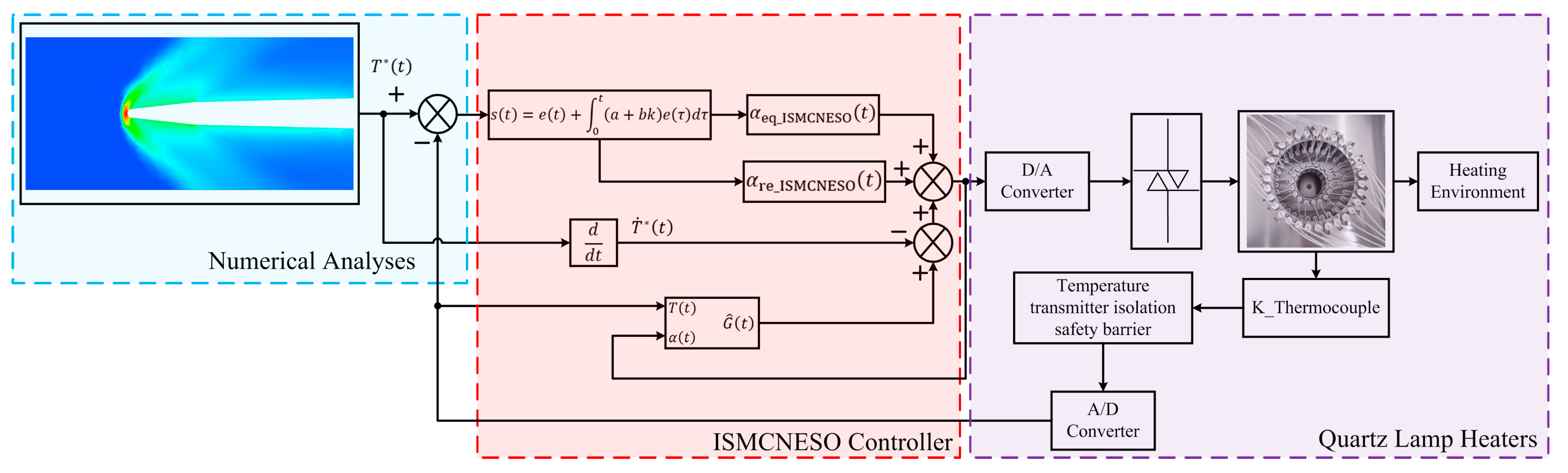
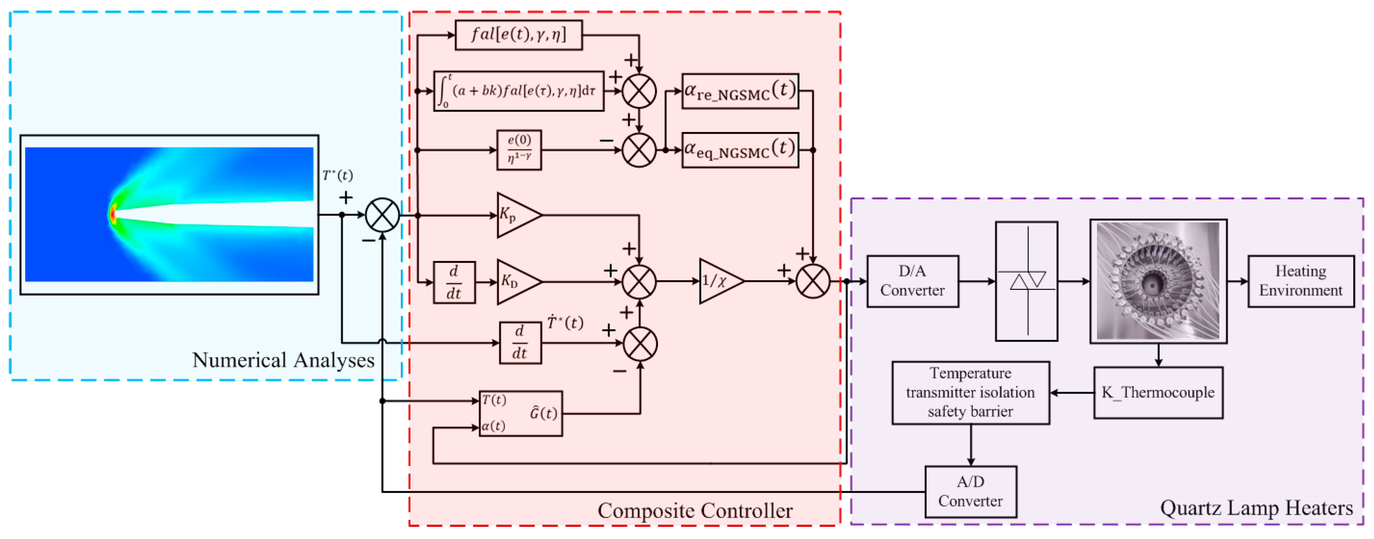
- The NESO is designed for the lumped disturbances observation and the NGSMC, an auxiliary controller of MFC, combines an integral sliding mode with a nonlinear function to achieve a stage of great tracking errors, fast response time, and strong robustness. Moreover, the NGSMC eliminates the reaching phase, suppressing chattering phenomena from the high-frequency switching motions.
- Instead of sign functions, the nonlinear function is integrated into NGSMC, alleviating steady state errors and saturation errors and achieves a goal: smaller errors corresponding to larger gains and larger errors corresponding to smaller gains.
- The comparative results demonstrate some superiorities of the proposed composite controller in terms of tracking errors and robustness.
2. Thermal-Structural Test with Quartz Lamp Heaters
3. Numerical Analyses
4. Control System
4.1. The System Dynamic Model of TSTQLs
4.2. Control Methods
4.2.1. NESO
4.2.2. Controller Design
5. Simulation Results
6. Conclusions
Author Contributions
Funding
Institutional Review Board Statement
Informed Consent Statement
Data Availability Statement
Acknowledgments
Conflicts of Interest
References
- Wang, Z.; Wang, H.; Ding, N.; Zhang, J.; Hu, B. Research on the development of hypersonic vehicle technology. Sci. Technol. Rev. 2021, 39, 59–67. [Google Scholar]
- Tachinina, O.M.; Lysenko, O.I.; Alekseeva, I.V. Algorithm for Operational Optimization of Two-Stage Hypersonic Unmanned Aerial Vehicle Branching Path. In Proceedings of the 5th IEEE International Conference on Methods and Systems of Navigation and Motion Control (MSNMC), Kyiv, Ukraine, 16–18 October 2018; IEEE: Piscataway, NJ, USA; pp. 11–15. [Google Scholar]
- Zhu, C.; Xu, G.; Wei, C.; Cai, D.; Yu, Y. Impact-Time-Control Guidance Law for Hypersonic Missiles in Terminal Phase. IEEE Access 2020, 8, 44611–44621. [Google Scholar] [CrossRef]
- Niculescu, M.L.; Cojocaru, M.G.; Pricop, M.V.; Fadgyas, M.C.; Stoican, M.G.; Pepelea, D. Hypersonic Gas Dynamics of a Marco Polo Reentry Capsule. In Proceedings of the International Conference of Numerical Analysis and Applied Mathematics (ICNAAM), Thessaloniki, Greece, 13–18 September 2018. [Google Scholar]
- Urzay, J. Supersonic Combustion in Air-Breathing Propulsion Systems for Hypersonic Flight. Annu. Rev. Fluid Mech. 2018, 50, 593–627. [Google Scholar] [CrossRef]
- D’Oriano, V.; Savino, R.; Visone, M. Aerothermodynamic study of a small hypersonic plane. Aircr. Eng. Aerosp. Technol. 2018, 90, 471–480. [Google Scholar] [CrossRef]
- Qin, X.; Shui, Y.; Wang, Y.; Wang, F.; Li, Q. Research on Aeroheating of Complicated Hypersonic Reentry Vehicles. In Proceedings of the 9th International Conference on Mechanical and Aerospace Engineering (ICMAE), Budapest, Hungary, 10–13 July 2018; IEEE: Piscataway, NJ, USA; pp. 136–140. [Google Scholar]
- Gong, C.-L.; Gou, J.-J.; Hu, J.-X.; Gao, F. A novel TE-material based thermal protection structure and its performance evaluation for hypersonic flight vehicles. Aerosp. Sci. Technol. 2018, 77, 458–470. [Google Scholar] [CrossRef]
- Lv, X.; Zhang, G.; Zhu, M.; Ouyang, H.; Shi, Z.; Bai, Z.; Alexandrov, I.V. Adaptive Neural Network Global Nonsingular Fast Terminal Sliding Mode Control for a Real Time Ground Simulation of Aerodynamic Heating Produced by Hypersonic Vehicles. Energies 2022, 15, 3284. [Google Scholar] [CrossRef]
- Liu, L.; Dai, G.; Zeng, L.; Wang, Z.; Gui, Y. Experimental Model Design and Preliminary Numerical Verification of Fluid-Thermal-Structural Coupling Problem. AIAA J. 2019, 57, 1715–1724. [Google Scholar]
- Shams, T.A.; Shah, S.I.A.; Ahmad, M.A. Capability Analysis of Global Hypersonic Wind Tunnel Facilities for Aerothermodynamic Investigations. In Proceedings of the 17th International Bhurban Conference on Applied Sciences and Technology (IBCAST), Natl Ctr Phys, Islamabad, Pakistan, 14–18 January 2020; pp. 481–501. [Google Scholar]
- Xu, X.; Shu, H.; Xie, F.; Wang, X.; Guo, L. Research progress on aerodynamic test technology of hypersonic wind tunnel for air-breathing aerocraft. J. Exp. Fluid Mech. 2018, 32, 29–40. [Google Scholar]
- Jiang, Z. Progresses on experimental techniques of hypersonic and high-enthalpy wind tunnels. Acta Aerodyn. Sin. 2019, 37, 347–355. [Google Scholar]
- Lin, L.; Wu, D.; Ren, H.; Zhu, F. Thermal shock fracture behavior of wave-transparent brittle materials in hypersonic vehicles under high thermal flux by digital image correlation. Opt. Express 2019, 27, 10269–10279. [Google Scholar] [CrossRef]
- Zhu, Y.; Zeng, L.; Dong, W.; Du, Y.; Gui, Y. Computational and Experimental Study on Quartz Lamp Array Heat Flux Distribution. J. Astronaut. 2017, 38, 1131–1138. [Google Scholar]
- Wu, D.; Gao, Z.; Wang, Y. Experimental Study on Fuzzy Control of Transient Aerodynamic Heat Flow of Missile. J. Beijing Univ. Aeronaut. Astronaut. 2002, 28, 682–684. [Google Scholar]
- Zhang, W.J.S.; Engineering, E. Research on control of heating system for aerodynamic heating simulation test. Adv. Mater. Res. 2005, 705, 528–533. [Google Scholar]
- Lan, T.; Lin, H.; Zhang, K. Fractional Order Iterative Learning Control Strategy for Quartz Lamp Radiation Aerodynamic Heating Experiment. J. Northwestern Polytech. Univ. 2017, 35, 26–31. [Google Scholar]
- Fliess, M.; Join, C. Model-free control. Int. J. Control 2013, 86, 2228–2252. [Google Scholar] [CrossRef] [Green Version]
- Zhang, X.; Wang, H.; Tian, Y.; Peyrodie, L.; Wang, X. Model-free based neural network control with time-delay estimation for lower extremity exoskeleton. Neurocomputing 2018, 272, 178–188. [Google Scholar] [CrossRef]
- Gao, P.; Lv, X.; Ouyang, H.; Mei, L.; Zhang, G. A Novel Model-Free Intelligent Proportional-Integral Supertwisting Nonlinear Fractional-Order Sliding Mode Control of PMSM Speed Regulation System. Complexity 2020, 2020, 8405453. [Google Scholar] [CrossRef]
- Wang, H.; Li, S.; Tian, Y.; Aitouche, A. Intelligent Proportional Differential Neural Network Control for Unknown Nonlinear System. Stud. Inform. Control 2016, 25, 445–452. [Google Scholar] [CrossRef] [Green Version]
- Liu, Y.; Jiang, B.; Lu, J.; Cao, J.; Lu, G. Event-Triggered Sliding Mode Control for Attitude Stabilization of a Rigid Spacecraft. Ieee Trans. Syst. Man Cybern.-Syst. 2020, 50, 3290–3299. [Google Scholar] [CrossRef]
- Lopac, N.; Bulic, N.; Vrkic, N. Sliding Mode Observer-Based Load Angle Estimation for Salient-Pole Wound Rotor Synchronous Generators. Energies 2019, 12, 1609. [Google Scholar] [CrossRef] [Green Version]
- Qiu, B.; Wang, G.; Fan, Y.; Mu, D.; Sun, X. Adaptive Sliding Mode Trajectory Tracking Control for Unmanned Surface Vehicle with Modeling Uncertainties and Input Saturation. Appl. Sci. 2019, 9, 1240. [Google Scholar] [CrossRef] [Green Version]
- Liu, Y.-C.; Laghrouche, S.; N’Diaye, A.; Cirrincione, M. Hermite neural network-based second-order sliding-mode control of synchronous reluctance motor drive systems. J. Frankl. Inst.-Eng. Appl. Math. 2021, 358, 400–427. [Google Scholar] [CrossRef]
- Soriano, L.A.; Rubio, J.d.J.; Orozco, E.; Cordova, D.A.; Ochoa, G.; Balcazar, R.; Cruz, D.R.; Meda-Campana, J.A.; Zacarias, A.; Gutierrez, G.J. Optimization of Sliding Mode Control to Save Energy in a SCARA Robot. Mathematics 2021, 9, 3160. [Google Scholar] [CrossRef]
- Rahman, A.U.; Zehra, S.S.; Ahmad, I.; Armghan, H. Fuzzy supertwisting sliding mode-based energy management and control of hybrid energy storage system in electric vehicle considering fuel economy. J. Energy Storage 2021, 37, 102468. [Google Scholar] [CrossRef]
- Li, S.; Wang, H.; Tian, Y.; Aitouch, A.; Klein, J. Direct power control of DFIG wind turbine systems based on an intelligent proportional-integral sliding mode control. ISA Trans. 2016, 64, 431–439. [Google Scholar] [CrossRef]
- Jiang, J.; Chen, H.; Cao, D.; Guirao, J.L.G. The global sliding mode tracking control for a class of variable order fractional differential systems. Chaos Solitons Fractals 2022, 154, 111674. [Google Scholar] [CrossRef]
- Saghafi Zanjani, M.; Mobayen, S. Anti-sway control of offshore crane on surface vessel using global sliding mode control. Int. J. Control 2022, 95, 2267–2278. [Google Scholar] [CrossRef]
- Wu, X.; Xu, K. Global sliding mode control for the underactuated translational oscillator with rotational actuator system. Proc. Inst. Mech. Eng. Part I-J. Syst. Control Eng. 2021, 235, 540–549. [Google Scholar] [CrossRef]
- Mofid, O.; Mobayen, S. Adaptive Finite-Time Backstepping Global Sliding Mode Tracker of Quad-Rotor UAVs Under Model Uncertainty, Wind Perturbation, and Input Saturation. IEEE Trans. Aerosp. Electron. Syst. 2022, 58, 140–151. [Google Scholar] [CrossRef]
- Tong, X.; Zhao, H.; Feng, G. Adaptive global Terminal Sliding Mode Control for Anti-Warship Missiles. In Proceedings of the 6th World Congress on Intelligent Control and Automation, Dalian, China, 21–23 June 2006; IEEE: Piscataway, NJ, USA; pp. 1962–1966. [Google Scholar]
- Lv, X.; Zhang, G.; Zhu, M.; Shi, Z.; Bai, Z.; Alexandrov, I.V. Aerodynamic Heating Ground Simulation of Hypersonic Vehicles Based on Model-Free Control Using Super Twisting Nonlinear Fractional Order Sliding Mode. Mathematics 2022, 10, 1664. [Google Scholar] [CrossRef]
- Sissenwine, N. U.S. committee on extension to the standard atmosphere. Nature 1962, 195, 133–134. [Google Scholar] [CrossRef]
- Han, J. From PID to Active Disturbance Rejection Control. IEEE Trans. Ind. Electron. 2009, 56, 900–906. [Google Scholar] [CrossRef]
- Yang, H.; Guo, M.; Xia, Y.; Sun, Z. Dual closed-loop tracking control for wheeled mobile robots via active disturbance rejection control and model predictive control. Int. J. Robust Nonlinear Control 2020, 30, 80–99. [Google Scholar] [CrossRef]
- Shyu, K.K.; Shieh, H.J. A new switching surface sliding-mode speed control for induction motor drive systems. IEEE Trans. Power Electron. 1996, 11, 660–667. [Google Scholar] [CrossRef]
- Li, T. Nonlinear Integral Sliding Mode Control Method Based on New Reaching Law. Control Eng. China 2019, 26, 2031–2035. [Google Scholar]


| H | T | a | P | R | M | |
|---|---|---|---|---|---|---|
| a | 31,272 | 227.922 | 302.6483 | 968 | 0.0148 | 0.61136 |
| b | 29,934 | 226.584 | 301.7587 | 1184 | 0.0182 | 0.768021 |
| c | 28,596 | 225.246 | 300.8664 | 1449 | 0.0224 | 0.924682 |
| d | 27,258 | 223.908 | 299.9715 | 1776 | 0.0276 | 1.081343 |
| e | 25,920 | 222.57 | 299.0738 | 2180 | 0.0341 | 1.238004 |
| f | 25,380 | 222.03 | 298.7108 | 2368 | 0.0372 | 1.394665 |
| g | 24,840 | 221.49 | 298.3473 | 2574 | 0.0405 | 1.551326 |
| h | 24,300 | 220.95 | 297.9834 | 2798 | 0.0441 | 1.707987 |
| i | 23,760 | 220.41 | 297.6191 | 3041 | 0.0481 | 1.864648 |
| j | 23,220 | 219.87 | 297.2543 | 3307 | 0.0524 | 2.021309 |
| k | 22,680 | 219.33 | 296.889 | 3597 | 0.0571 | 2.17797 |
| l | 22,140 | 218.79 | 296.5233 | 3913 | 0.0623 | 2.277316 |
| m | 21,600 | 218.25 | 296.1572 | 4258 | 0.068 | 2.376662 |
| n | 21,060 | 217.71 | 295.7906 | 4634 | 0.0742 | 2.476008 |
| o | 20,520 | 217.17 | 295.4235 | 5044 | 0.0809 | 2.575354 |
| p | 19,980 | 216.65 | 295.0696 | 5492 | 0.0883 | 2.6747 |
| q | 19,440 | 216.65 | 295.0696 | 5980 | 0.0962 | 2.774046 |
| r | 18,900 | 216.65 | 295.0696 | 6512 | 0.1047 | 2.873392 |
| s | 18,360 | 216.65 | 295.0696 | 7091 | 0.114 | 2.972738 |
| t | 17,820 | 216.65 | 295.0696 | 7721 | 0.1242 | 3.072084 |
| u | 17,280 | 216.65 | 295.0696 | 8407 | 0.1352 | 3.17143 |
| v | 16,861 | 216.65 | 295.0696 | 8981 | 0.1444 | 3.270776 |
| w | 16,450 | 216.65 | 295.0696 | 9583 | 0.1541 | 3.370122 |
| x | 16,040 | 216.65 | 295.0696 | 10,223 | 0.1644 | 3.469468 |
| y | 15,629 | 216.65 | 295.0696 | 10,907 | 0.1754 | 3.568814 |
| z | 15,219 | 216.65 | 295.0696 | 11,636 | 0.1871 | 3.66816 |
| A | 14,809 | 216.65 | 295.0696 | 12,413 | 0.1996 | 3.821 |
| B | 14,398 | 216.65 | 295.0696 | 13,244 | 0.213 | 4.212653 |
| C | 13,988 | 216.65 | 295.0696 | 14,129 | 0.2272 | 4.614305 |
| D | 13,577 | 216.65 | 295.0696 | 15,075 | 0.2424 | 5.015958 |
| Min | Max | Average | Standard Deviation | |
|---|---|---|---|---|
| 0° | 0.49732 | 0.99999 | 0.96312 | 0.036722 |
| 5° | 0.39539 | 0.99997 | 0.96445 | 0.037045 |
| 10° | 0.47993 | 0.99999 | 0.96397 | 0.037951 |
| Pressure-Velocity Coupling | Spatial Discretization | |||||||
|---|---|---|---|---|---|---|---|---|
| Scheme | Gradient | Pressure | Density | Momentum | Turbulent Kinetic Energy | Specific Dissipation Rate | Energy | |
| 0° | Coupled | Least Squares Cell Based | Second Order | Second Order Upwind | Second Order Upwind | First Order Upwind | First Order Upwind | Second Order Upwind |
| 5° | Coupled | Green-Gauss Cell Based | Second Order | Second Order Upwind | Second Order Upwind | First Order Upwind | First Order Upwind | Second Order Upwind |
| 10° | Coupled | Least Squares Cell Based | Second Order | Second Order Upwind | Second Order Upwind | First Order Upwind | First Order Upwind | Second Order Upwind |
| Pseudo-Transient Explicit Relaxation Factors | ||||||||
|---|---|---|---|---|---|---|---|---|
| Pressure | Momentum | Density | Body Forces | Turbulent inetic Energy | Specific issipation Rate | Turbulent Viscosity | Energy | |
| 0° | 0.5 | 0.5 | 1 | 1 | 0.75 | 0.75 | 1 | 0.75 |
| 5° | 0.5 | 0.5 | 0.8 | 1 | 0.75 | 0.75 | 1 | 0.75 |
| 10° | 0.5 | 0.5 | 1 | 0.9 | 0.75 | 0.75 | 1 | 0.75 |
| SSE | R-Square | Adjusted R-Square | RMSE | |
|---|---|---|---|---|
| Wall 0_0 mm | 12,600 | 0.9962 | 0.9954 | 22.91 |
| Wall 0_3 mm | 9883 | 0.9949 | 0.9939 | 20.29 |
| Wall 0_6 mm | 11,360 | 0.9911 | 0.9882 | 22.72 |
| Wall 1_5 mm | 19,000 | 0.9904 | 0.9884 | 28.13 |
| Wall 1_45 mm | 3780 | 0.9963 | 0.9951 | 13.11 |
| Wall 1_85 mm | 4263 | 0.9948 | 0.9937 | 13.33 |
| Wall 2_5 mm | 15,250 | 0.9878 | 0.9853 | 25.21 |
| Wall 2_45 mm | 2293 | 0.9958 | 0.9949 | 9.773 |
| Wall 2_85 mm | 7589 | 0.9795 | 0.9753 | 17.78 |
| Symbol | Unit | Description |
|---|---|---|
| V | the input voltage of QLH | |
| rad | the SCR conduction angle | |
| V | the supply voltage of QLH | |
| rad | the phase angle | |
| W | the input electric power of QLH | |
| Ω | the total resistance of QLH | |
| the specific heat capacity of quartz lamp filament | ||
| the mass of quartz lamp filament | ||
| K | the current temperature of QLH | |
| K | the previous QLH’s temperature of the time interval | |
| s | the time interval | |
| the surface area of quartz lamp tube | ||
| the heat convection coefficient of QLH | ||
| the heat conduction coefficient of QLH | ||
| the heat radiation blackness coefficient of QLH | ||
| the Stephen Boltzmann’s constant | ||
| the angle coefficient |
| ISMCNESO Controller | NGSMCNESO Controller | Composite Controller | ||||
|---|---|---|---|---|---|---|
| RMSE | MAX | RMSE | MAX | RMSE | MAX | |
| Wall 0_0 mm | 0.486 | 1.000700 | 0.161 | 0.410 | 0.00682 | 0.174 |
| Wall 0_3 mm | 0.491 | 1.00300 | 0.132 | 0.431 | 0.00634 | 0.192 |
| Wall 0_6 mm | 0.257 | 0.924 | 0.109 | 0.400 | 0.00235 | 0.0628 |
| Wall 1_5 mm | 0.534 | 1.0100 | 0.117 | 0.402 | 0.00532 | 0.135 |
| Wall 1_45 mm | 0.136 | 1.0531 | 0.103 | 0.400 | 0.00204 | 0.0993 |
| Wall 1_85 mm | 0.116 | 1.0519 | 0.0968 | 0.383 | 0.00202 | 0.0580 |
| Wall 2_5 mm | 0.162 | 1.0678 | 0.111 | 0.406 | 0.00291 | 0.0799 |
| Wall 2_45 mm | 0.118 | 1.00392 | 0.0887 | 0.346 | 0.00277 | 0.0574 |
| Wall 2_85 mm | 0.0832 | 0.922 | 0.0759 | 0.393 | 0.00283 | 0.0520 |
Publisher’s Note: MDPI stays neutral with regard to jurisdictional claims in published maps and institutional affiliations. |
© 2022 by the authors. Licensee MDPI, Basel, Switzerland. This article is an open access article distributed under the terms and conditions of the Creative Commons Attribution (CC BY) license (https://creativecommons.org/licenses/by/4.0/).
Share and Cite
Lv, X.; Zhang, G.; Wang, G.; Zhu, M.; Shi, Z.; Bai, Z.; Alexandrov, I.V. Numerical Analyses and a Nonlinear Composite Controller for a Real-Time Ground Aerodynamic Heating Simulation of a Hypersonic Flying Object. Mathematics 2022, 10, 3022. https://doi.org/10.3390/math10163022
Lv X, Zhang G, Wang G, Zhu M, Shi Z, Bai Z, Alexandrov IV. Numerical Analyses and a Nonlinear Composite Controller for a Real-Time Ground Aerodynamic Heating Simulation of a Hypersonic Flying Object. Mathematics. 2022; 10(16):3022. https://doi.org/10.3390/math10163022
Chicago/Turabian StyleLv, Xiaodong, Guangming Zhang, Gang Wang, Mingxiang Zhu, Zhihan Shi, Zhiqing Bai, and Igor V. Alexandrov. 2022. "Numerical Analyses and a Nonlinear Composite Controller for a Real-Time Ground Aerodynamic Heating Simulation of a Hypersonic Flying Object" Mathematics 10, no. 16: 3022. https://doi.org/10.3390/math10163022
APA StyleLv, X., Zhang, G., Wang, G., Zhu, M., Shi, Z., Bai, Z., & Alexandrov, I. V. (2022). Numerical Analyses and a Nonlinear Composite Controller for a Real-Time Ground Aerodynamic Heating Simulation of a Hypersonic Flying Object. Mathematics, 10(16), 3022. https://doi.org/10.3390/math10163022