Smoothed Quantile Regression with Factor-Augmented Regularized Variable Selection for High Correlated Data

Abstract

This paper studies variable selection for the data set, which has heavy-tailed distribution and high correlations within blocks of covariates. Motivated by econometric and financial studies, we consider using quantile regression to model the heavy-tailed distribution data. Considering the case where the covariates are high dimensional and there are high correlations within blocks, we use the latent factor model to reduce the correlations between the covariates and use the conquer to obtain the estimators of quantile regression coefficients, and we propose a consistency strategy named factor-augmented regularized variable selection for quantile regression (Farvsqr). By principal component analysis, we can obtain the latent factors and idiosyncratic components; then, we use both as predictors instead of the covariates with high correlations. Farvsqr transforms the problem from variable selection with highly correlated covariates to that with weakly correlated ones for quantile regression. Variable selection consistency is obtained under mild conditions. Simulation study and real data application demonstrate that our method is better than the common regularized M-estimation LASSO.

1. Introduction

Along with the continuous development of data collection and storage technology, data sets that present high dimensions and high correlations within blocks of variables can cause some new research problems in economics, finance, genomics, statistics, machine learning, etc. Because for such data, we need to make a variable selection in highly correlated variables.

There has been significant research into variable selection methods, and many variable selection methods have been developed, such as the regularized M-estimation method, which includes the LASSO [1], SCAD [2], elastic net [3], and the Dantzig selector [4]. There are many references to the regularized M-estimation method’s theoretical properties and algorithmic studies, including [5,6,7,8,9,10,11,12,13,14].

Most existing variable selection methods assume that the covariates are cross-sectionally weakly correlated, even, and serially independent. However, these assumptions are easily invalid in the data sets, which present high dimensions and high correlations within blocks of covariates, such as economic and financial data sets. For example, economics studies [15,16,17] show a strong correlation within blocks of covariates. In order to deal with the problem, Fan et al. proposed factor-adjusted variable selection for mean regression [18].

However, mean regression cannot simultaneously fit the skew and heavy-tailed data; mean regression is not robust against the outliers. Koenker and Bassett [19] proposed quantile regression (QR) to model the relationship between the response y and the covariates $\mathbf{x}$. Compared to the mean regression, QR has two significant advantages: (i) QR can be used to model the entire conditional distribution of y given $\mathbf{x}$, and thus, it provides insightful information about the relationship between y and $\mathbf{x}$. The conditional distribution function of Y given $\mathbf{x}$ is $F\left(y\right|\mathbf{x})=P(Y\le y\left|\mathbf{x}\right)$. For $0<\tau <1$, the $\tau -$ th conditional quantile of Y given $\mathbf{x}$ is defined as $Q_{Y|\mathbf{x}}\left(\tau \right)=inf\{t:F\left(t\right|\mathbf{x})\ge \tau \}$. (ii) QR is robust against outliers and can be used to model the response in which distribution is skewed or heavy-tailed without correct error assumption. These two advantages make QR an appealing method to reflect data information that is difficult for the mean regression. The researchers can refer to Koenker [20] and Koenker et al. [21] for a comprehensive overview of methods, theory, computation, and many extensions of QR.

Ando and Tsay [22] proposed factor-augmented predictors for quantile regression, but the model did not contain the idiosyncratic components of the covariates, so it will cause an information loss of explanatory variables. So, we refer to Fan et al. [18] and propose the factor-augmented regularized variable selection (Farvsqr) for quantile regression to overcome the problems caused by the correlations within the covariates. As usual, let us assume that the i-th observation covariates ${\mathbf{x}}_i={\left(x_{i1},\cdots ,x_{ip}\right)}^{\mathrm{T}}$ follow an approximate factor model,

$${\mathbf{x}}_i=\Lambda f_i+{\mathit{ϵ}}_i,$$

(1)

where $f_i$ is a $k\times 1$ vector of latent factors, $\Lambda$ is a $p\times k$ loading matrix, and ${\mathit{ϵ}}_i$ is a $p\times 1$ vector of idiosyncratic components or errors which are independent of $f_i$.

The factor model has become one of the most popular and powerful tools in multivariate statistics and deeply impacted biology [23,24,25], economics, and finance [15,16,26]. Chamberlain and Rothschild [27] first proposed using principal component analysis (PCA) to solve the approximate factor model’s latent factors and loading matrix. Subsequently, much literature explores the factor model using the PCA method [28,29,30,31,32]. In our paper, we will use the PCA to obtain the estimators of $\Lambda$, $f_i$, and ${\mathit{ϵ}}_i$.

The process of Farvsqr is first to estimate model (1) and obtain the independent or low-correlated estimators of $f_i$ and ${\mathit{ϵ}}_i$. Then, we replace the high correlation covariates ${\mathbf{x}}_i$ with the estimators $f_i$ and ${\mathit{ϵ}}_i$. The second step is to solve a common regularized loss function. In this paper, we study Farvsqr by giving the specific parameter-solving process and the theoretical properties. Moreover, both simulation and real data application studies are presented.

The main contribution of our paper is to generalize the factor-adjusted regularized variable selection of mean regression to the quantile regression to accommodate the skew and heavy-tailed data. Section 2 introduces the smoothed quantile regression and the approximate factor models. Section 3 introduces the variable selection methodology of Farvsqr. Section 4 presents the general theoretical results. Section 5 provides simulation studies, and Section 6 applies our model to the Quarterly Database for Macroeconomic Research (FRED-QD).

2. Quantile Regression and Approximate Factor Model

2.1. Notations

Now, we will give some notations that will be used throughout the paper. Let ${\mathbf{I}}_n$ denote the $n\times n$ identity matrix; $\mathbf{0}$ denotes the $n\times m$ zero matrix; ${\mathbf{0}}_n$ and ${\mathbf{1}}_n$ denote the zero vector and one vector in ${\mathbb{R}}^n$, respectively. For a matrix $\mathbf{W}$, let ${\parallel \mathbf{W}\parallel }_{max}=ma{x}_{i,j}\parallel W_{ij}\parallel$ denote its max norm, while ${\parallel \mathbf{W}\parallel }_F$ and ${\parallel \mathbf{W}\parallel }_p$ denote its Frobenius and induced p-norms, respectively. Let ${\lambda }_{min}\left(\mathbf{W}\right)$ denote the minimum eigenvalue of $\mathbf{W}$ if it is symmetric. For $\mathbf{W}\in {\mathbb{R}}^{n\times m}$, $I\in \left[n\right]$ and $J\in \left[m\right]$, define ${\mathbf{W}}_{IJ}={\left({\mathbf{W}}_{ij}\right)}_{i\in I,j\in J}$, ${\mathbf{W}}_{I·}={\left({\mathbf{W}}_{ij}\right)}_{i\in I,j\in \left[m\right]}$, ${\mathbf{W}}_{·J}={\left({\mathbf{W}}_{ij}\right)}_{i\in \left[n\right],j\in J}$. For a vector $\mathbf{w}\in {\mathbb{R}}^p$ and $L\subseteq \left[p\right]$, define ${\mathbf{w}}_L={\left({\mathbf{w}}_i\right)}_{i\in L}$ to be its subvector. Let ∇ and ${\nabla }^2$ be the gradient and Hessian operators. For $f:{\mathbb{R}}^p\to \mathbb{R}$ and $I,J\in \left[p\right]$, define ${\nabla }_{I}f\left(x\right)={\left(\nabla f\left(x\right)\right)}_I$ and ${\nabla }_{IJ}^{2}f\left(x\right)={\left({\nabla }^{2}f\left(x\right)\right)}_{IJ}$. Let $N(\mathit{\mu },\mathbf{\Sigma })$ denote the normal distribution with mean $\mathit{\mu }$ and covariance matrix $\mathbf{\Sigma }$.

2.2. Regularized M-Estimator for Quantile Regression

This subsection will begin with high-dimensional regression problems with heavy-tailed data. Let $\mathbf{y}=(y_1,\cdots ,y_n)$ be the response vector, ${\mathbf{x}}_i={(x_{i1},\cdots ,x_{ip})}^{\mathrm{T}}$, $i=1,\cdots ,n$ be the p-dimensional vectors of the explanatory variables. Let $\mathbf{X}=\left({\mathbf{1}}_n,{({\mathbf{x}}_1,\cdots ,{\mathbf{x}}_n)}^{\mathrm{T}}\right)\in {\mathbb{R}}^{n\times (p+1)}$ be the design matrix and $\mathbf{y}={(y_1,y_2,\cdots ,y_n)}^{\mathrm{T}}\in {\mathbb{R}}^n$ be the response vector. Let ${\mathbf{X}}_1={\left({\mathbf{x}}_1,\cdots ,{\mathbf{x}}_n\right)}^{\mathrm{T}}\in {\mathbb{R}}^{n\times p}$ be the matrix including n samples of the p-dimensional vector.

In this paper, we will fit the heavy-tailed data with quantile regression. Let $F_{y_i|{\mathbf{x}}_i}$ be the conditional cumulative distribution function of $y_i$ given ${\mathbf{x}}_i$. Under the linear quantile regression assumption, the $\tau$th conditional quantile function is defined as

$$F_{y_i|{\mathbf{x}}_i}^{-1}\left(\tau \right)={\beta }_0^{*}\left(\tau \right)+\sum _{j=1}^p{\beta }_j^{*}\left(\tau \right)x_{ij}=\left(1,{\mathbf{x}}_i^{\mathrm{T}}\right){\mathit{\beta }}^{*}\left(\tau \right)$$

(2)

where the quantile $\tau \in \left(0,1\right)$, ${\mathit{\beta }}^{*}\left(\tau \right)={\left({\beta }_0^{*}\left(\tau \right),{\beta }_1^{*}\left(\tau \right),\cdots ,{\beta }_p^{*}\left(\tau \right)\right)}^{\mathrm{T}}$ is the true coefficients of the quantile regression that changes with the quantile $\tau$. For the convenience of writing, we will omit the $\tau$ given in the following.

Under the linear quantile regression assumption, the common regression coefficient estimator at a given $\tau$ can be given as [19]

$$\widehat{\mathit{\beta }}\in argmi{n}_{\mathit{\beta }\in {\mathbb{R}}^{p+1}}R\left(\mathbf{y},\mathbf{X}\mathit{\beta }\right)=argmi{n}_{\mathit{\beta }\in {\mathbb{R}}^{p+1}}\frac{1}{n}\sum _{i=1}^n{\rho }_{\tau }(y_i-\left(1,{\mathbf{x}}_i^{\mathrm{T}}\right)\mathit{\beta }),$$

(3)

where ${\rho }_{\tau }\left(u\right)=u(\tau -{\mathbf{I}}_{\left(u\le 0\right)})$ is the check function, ${\mathbf{I}}_{\left(u\le 0\right)}$ is the indicator function, and $\tau$ is the quantile. However, as we know, the check function is not differentiable, which is very different from other widely used objective functions. The non-differentiable has two obvious disadvantages: (i) theoretical analysis of the estimator is very difficult; and (ii) gradient-based optimization methods cannot be used. So, He et al. [33] proposed a smoothed quantile regression for large-scale inference, which is denoted as conquer (convolution-type smoothed quantile regression). He et al. [33] concluded that the conquer method could improve estimation accuracy and computational efficiency for fitting large-scale linear quantile regression models rather than by minimizing the check function (3). So, in our paper, we will use the conquer to estimate the quantile regression. The estimator is given by

$$\widehat{\mathit{\beta }}\in argmi{n}_{\mathit{\beta }\in {\mathbb{R}}^{p+1}}R\left(\mathbf{y},\mathbf{X}\mathit{\beta }\right)=argmi{n}_{\mathit{\beta }\in {\mathbb{R}}^{p+1}}\frac{1}{n}\sum _{i=1}^n{\mathcal{L}}_h(y_i-\left(1,{\mathbf{x}}_i^{\mathrm{T}}\right)\mathit{\beta })$$

(4)

where ${\mathcal{L}}_h\left(v\right)=({\rho }_{\tau }*K_h)\left(v\right)={\int }_{-\infty }^{\infty }{\rho }_{\tau }\left(w\right)K_h(w-v)dw$, $K(·)$ is a symmetric and non-negative kernel function in which the integral is 1, and h is the bandwidth. Referring to He et al. [33], we have the definition:

$$K_h\left(v\right)=\frac{1}{h}K(v/h),{\mathcal{K}}_h\left(v\right)=\mathcal{K}(v/h),\mathcal{K}\left(v\right)={\int }_{-\infty }^{v}K\left(w\right)dw,v\in \mathbb{R}.$$

The conquer function $R\left(\mathbf{y},\mathbf{X}\mathit{\beta }\right)$ is twice continuously differentiable relative to $\mathit{\beta }$; the gradient matrix and hessian matrix are as follows:

$$\begin{array}{cc}\hfill & \nabla R\left(\mathbf{y},\mathbf{X}\mathit{\beta }\right)=\frac{1}{n}\sum _{i=1}^n\{{\mathcal{K}}_h\left(\left(1,{\mathbf{x}}_i^{\mathrm{T}}\right)\mathit{\beta }-y_i\right)-\tau \}{\left(1,{\mathbf{x}}_i^{\mathrm{T}}\right)}^{\mathrm{T}},\hfill \\ \hfill & {\nabla }^{2}R\left(\mathbf{y},\mathbf{X}\mathit{\beta }\right)=\frac{1}{n}\sum _{i=1}^n{K}_h\left(\left(1,{\mathbf{x}}_i^{\mathrm{T}}\right)\mathit{\beta }-y_i\right){\left(1,{\mathbf{x}}_i^{\mathrm{T}}\right)}^{\mathrm{T}}\left(1,{\mathbf{x}}_i^{\mathrm{T}}\right)\hfill \end{array}$$

When $\mathit{\beta }={({\beta }_0,{\beta }_1,\cdots ,{\beta }_p)}^{\mathrm{T}}$ is a sparse vector, it is common to estimate $\mathit{\beta }$ through the regularized M-estimator as the following:

$$\begin{array}{cc}\hfill & \widehat{\mathit{\beta }}\in argmi{n}_{\mathit{\beta }\in {\mathbb{R}}^{p+1}}R\left(\mathbf{y},\mathbf{X}\mathit{\beta }\right)+\lambda Q\left(\mathit{\beta }\right)\hfill \\ \hfill & =argmi{n}_{\mathit{\beta }\in {\mathbb{R}}^{p+1}}\frac{1}{n}\sum _{i=1}^n{\mathcal{L}}_h(y_i-\left(1,{\mathbf{x}}_i^{\top }\right)\mathit{\beta })+\lambda Q\left(\mathit{\beta }\right)\hfill \end{array}$$

(5)

We expect that the estimator of (5) satisfies two formulas: $\parallel \widehat{\mathit{\beta }}-{\mathit{\beta }}^{*}\parallel \stackrel{P}{\to }0$ for some norm $\parallel ·\parallel$ and $P(supp\left(\widehat{\mathit{\beta }}\right)=supp\left({\mathit{\beta }}^{*}\right))\to 1$ as $n\to \infty$. Zhao and Yu [9] studied the LASSO estimator for a sparse linear model and showed that there exists an irrepresentable condition that is sufficient and almost necessary for two formulas when we assume $supp\left({\mathit{\beta }}^{*}\right)=\left[l\right]=L$. Let ${\left(\mathbf{X}\right)}_L$ and ${\left(\mathbf{X}\right)}_{L^c}$ denote the submatrices of $\mathbf{X}$, which are the first l and the rest $(p+1-l)$ of the columns, respectively. Then, the irrepresentable condition is:

$${\parallel \left(X\right)}_{L^c}^{\top }{\left(X\right)}_L{\left[{\left(X\right)}_L^{\mathrm{T}}{\left(X\right)}_L\right]}^{-1}{\parallel }_{\infty }\le 1-\gamma$$

(6)

where $\gamma \in (0,1)$, but when the explanatory variables strongly correlate with the blocks, the irrepresentable condition will be easily invalid [18].

2.3. Approximate Factor Model

When there exist strong correlations between the covariates ${\mathbf{x}}_i$, in order to estimate the parameters $\mathit{\beta }$, the common method is the latent factor model. There are many papers in the literature that studied the latent factor model in econometrics and statistics [15,16,18,30,34].

As usual, let us assume that ${\mathbf{x}}_i\subseteq {\mathbb{R}}^p,i=1,\cdots ,n$ follows the approximate factor model (1). As we know, the ${\mathbf{x}}_i,i=1,\cdots ,n$ are the only observed variables; we need to estimate $\mathbf{\Lambda },{\mathbf{f}}_i,{\mathit{ϵ}}_i,i=1,\cdots ,n$. Generally, it is assumed that k is independent of n [18]. Let $\mathbf{F}={({\mathbf{f}}_1,\cdots ,{\mathbf{f}}_n)}^{\mathrm{T}}\in {\mathbb{R}}^{n\times k}$ be the latent factors matrix, and $\mathit{\epsilon }={({\mathit{ϵ}}_1,\cdots ,{\mathit{ϵ}}_n)}^{\mathrm{T}}\in {\mathbb{R}}^{n\times p}$ is the errors matrix. Then, Equation (1) can be written in a matrix as the following:

$${\mathbf{X}}_1=\mathbf{F}{\mathbf{\Lambda }}^{\mathrm{T}}+\mathit{\epsilon }.$$

(7)

Here, we need to note that ${\mathbf{x}}_i={(x_{i1},\cdots ,x_{ip})}^{\mathrm{T}},i=1,\cdots ,n$ have a strong correlation within the blocks, not including the intercept, so the matrix form of the latent factor model is ${\mathbf{X}}_1$ but not $\mathbf{X}$. We impose the basic assumption for the latent factor model to identify the model as Assumption 1 [18].

Assumption 1.

Assume that $cov\left({\mathbf{f}}_i\right)={\mathbf{I}}_k$, ${\mathbf{\Lambda }}^{\mathrm{T}}\mathbf{\Lambda }$ is diagonal, and all the eigenvalues of ${\mathbf{\Lambda }}^{\mathrm{T}}\mathbf{\Lambda }/p$ are bounded away from 0 and ∞ as $p\to \infty$.

3. Factor-Augmented Regularized Variable Selection

3.1. Methodology

Let ${\mathbf{\Lambda }}_0={({\mathbf{0}}_k,{\mathbf{\Lambda }}^{\mathrm{T}})}^{\mathrm{T}}\in {\mathbb{R}}^{\left(p+1\right)\times k}$, and ${\mathit{\epsilon }}_1=\left({\mathbf{1}}_n,\mathit{\epsilon }\right)\in {\mathbb{R}}^{n\times (p+1)}$. With the approximate factor model (7), we have $\mathbf{X}=\mathbf{F}{\mathbf{\Lambda }}_0^{\mathrm{T}}+{\mathit{\epsilon }}_1$, so we can obtain:

$$\mathbf{X}\mathit{\beta }=\mathbf{F}{\mathbf{\Lambda }}_0^{\mathrm{T}}\mathit{\beta }+{\mathit{\epsilon }}_1\mathit{\beta }=\mathbf{F}\mathit{\alpha }+{\mathit{\epsilon }}_1\mathit{\beta },$$

(8)

where $\mathit{\alpha }={\mathbf{\Lambda }}_0^{\mathrm{T}}\mathit{\beta }\in {\mathbb{R}}^k$. So, the regularized variable selection (5) can be written as:

$$\begin{array}{cc}\hfill & \widehat{\mathit{\beta }}\in argmi{n}_{\mathit{\beta }\in {\mathbb{R}}^{p+1},\mathit{\alpha }={\mathbf{\Lambda }}_0^{\mathrm{T}}\mathit{\beta }\in {\mathbb{R}}^k}R\left(\mathbf{y},\mathbf{X}\mathit{\beta }\right)+\lambda Q\left(\mathit{\beta }\right)\hfill \\ \hfill & =argmi{n}_{\mathit{\beta }\in {\mathbb{R}}^{p+1},\mathit{\alpha }={\mathbf{\Lambda }}_0^{\mathrm{T}}\mathit{\beta }\in {\mathbb{R}}^k}\frac{1}{n}\sum _{i=1}^n{\mathcal{L}}_h(y_i-(1,{\mathit{ϵ}}_i^{\mathrm{T}})\mathit{\beta }-{\mathbf{f}}_i^{\mathrm{T}}\mathit{\alpha })+\lambda Q\left(\mathit{\beta }\right)\hfill \end{array}$$

(9)

We need to estimate the coefficient of ${\mathbf{x}}_i,i=1,\cdots ,n$, namely $\mathit{\beta }$, so we consider $\mathit{\alpha }$ as the nuisance parameter. Now, let us consider a new estimator without the constraint $\mathit{\alpha }={\mathbf{\Lambda }}_0^{\mathrm{T}}\mathit{\beta }$,

$$\begin{array}{cc}\hfill & \widehat{\mathit{\beta }}\in argmi{n}_{\mathit{\beta }\in {\mathbb{R}}^{p+1},\mathit{\alpha }\in {\mathbb{R}}^k}R\left(\mathbf{y},\mathbf{X}\mathit{\beta }\right)+\lambda Q\left(\mathit{\beta }\right)\hfill \\ \hfill & =argmi{n}_{\mathit{\beta }\in {\mathbb{R}}^{p+1},\mathit{\alpha }\in {\mathbb{R}}^k}\frac{1}{n}\sum _{i=1}^n{\mathcal{L}}_h(y_i-(1,{\mathit{ϵ}}_i^{\mathrm{T}})\mathit{\beta }-{\mathbf{f}}_i^{\mathrm{T}}\mathit{\alpha })+\lambda Q\left(\mathit{\beta }\right)\hfill \end{array}$$

(10)

From Equation (10), we can see that the vector ${({\mathit{ϵ}}_i^{\mathrm{T}},{\mathbf{f}}_i^{\mathrm{T}})}^{\mathrm{T}}$ can be considered as the new explanatory variables. In other words, we lift the covariate space from $R^{p+1}$ to $R^{p+1+k}$ with the latent factor model, and the highly dependent covariates ${\mathbf{x}}_i$ are replaced by weakly dependent ${({\mathit{ϵ}}_i^{\mathrm{T}},{\mathbf{f}}_i^{\mathrm{T}})}^{\mathrm{T}}$.

We have the following lemma, whose proof is given in Appendix A:

Lemma 1.

Consider the model (2), let $R\left(\mathbf{y},\mathbf{X}\mathit{\beta }\right)=\frac{1}{n}{\sum }_{i=1}^n{\mathcal{L}}_h(y_i-\left(1,{\mathbf{x}}_i^{\mathrm{T}}\right)\mathit{\beta })$, ${\eta }_i={\mathcal{K}}_h\left(\left(1,{\mathbf{x}}_i^{\mathrm{T}}\right){\mathit{\beta }}^{*}-y_i\right)-\tau$ and ${\mathbf{v}}_i={(1,{\mathit{ϵ}}_i^{\mathrm{T}},{\mathbf{f}}_i^{\mathrm{T}})}^{\mathrm{T}}\in {\mathbb{R}}^{p+1+k}$. If $E\left({\eta }_i{\mathbf{v}}_i\right)={\mathbf{0}}_{p+1+k}$, then

$$\left({\mathit{\beta }}^{*},{\mathbf{\Lambda }}_0^{\mathrm{T}}{\mathit{\beta }}^{*}\right)=argmi{n}_{\mathit{\beta }\in {\mathbb{R}}^{p+1},\mathit{\alpha }\in {\mathbb{R}}^k}E\left[R\left(\mathbf{y},\mathbf{F}\mathit{\alpha }+{\mathit{\epsilon }}_1\mathit{\beta }\right)\right].$$

(11)

By the latent factor model, $(\mathit{\epsilon },\mathbf{F})$ has a much weaker correlation than ${\mathbf{X}}_1$. So, we can calculate the estimators by the following two steps:

• Let ${\mathbf{X}}_1\in {\mathbb{R}}^{n\times p}$ be the design matrix with strong cross-section correlations. Fit the approximate factor model (7), and the estimators of $\mathbf{\Lambda },\mathbf{F}$, and $\mathit{\epsilon }$ are denoted as $\widehat{\mathbf{\Lambda }},\widehat{\mathbf{F}},$ and $\widehat{\mathit{\epsilon }}$. This paper will use the principal component analysis (PCA) to estimate all the parameters in the latent factor model. Regarding PCA, the references such as Bai [28] and Fan et al. [18,30] are available. More specifically, the columns of $\widehat{\mathbf{F}}/\sqrt{n}$ are the eigenvectors of ${\mathbf{X}}_1{\mathbf{X}}_1^{\mathrm{T}}$ corresponding to the top k eigenvalues, $\widehat{\mathbf{\Lambda }}=\frac{1}{n}{\mathbf{X}}^{\mathrm{T}}\widehat{\mathbf{F}}$.
• Define $\widehat{\mathbf{V}}=\left({\mathbf{1}}_n,\widehat{\mathbf{\epsilon }},\widehat{\mathbf{F}}\right)\in {\mathbb{R}}^{n\times (p+1+k)}$ and $\mathit{\theta }={\left({\mathit{\beta }}^{\mathrm{T}},{\mathit{\alpha }}^{\mathrm{T}}\right)}^{\mathrm{T}}\in {\mathbb{R}}^{p+1+k}$. Then, $\widehat{\mathit{\beta }}$ is obtained from the first $p+1$ entries of the estimator vector of $\mathit{\theta }$.

  $$\begin{array}{cc}\hfill & \widehat{\mathit{\theta }}\in argmi{n}_{\mathit{\theta }\in {\mathbb{R}}^{p+1+k}}R(\mathbf{y},\widehat{\mathbf{V}}\mathit{\theta })+\lambda Q\left({\mathit{\theta }}_{[p+1]}\right)\hfill \\ \hfill & =argmi{n}_{\mathit{\theta }\in {\mathbb{R}}^{p+1+k}}\frac{1}{n}\sum _{i=1}^n{\mathcal{L}}_h(y_i-{\widehat{\mathbf{v}}}_i^{\mathrm{T}}\mathit{\theta })+\lambda Q\left({\theta }_{[p+1]}\right),\hfill \end{array}$$

  (12)

  where ${\widehat{\mathbf{v}}}_i^{\mathrm{T}}$ is the i-th row of the matrix $\widehat{\mathbf{V}}$.

We call the above two-step method as the factor-augmented regularized variable selection for quantile regression (Farvsqr). We successfully changed the quantile variable selection with highly correlated covariates $\mathbf{X}$ in (5) to quantile variable selection with weakly correlated or uncorrelated ones by the latent factor model in (12). Formula (12) is a convex function that can be minimized via the method conquer proposed by He et al. [33].

3.2. Selection Method of $\lambda$

Throughout all the study, the tuning parameter $\lambda$ is selected by 10-fold cross-validation. First, we are given an equally spaced sequence of size 50 with the range from 0.05 to 2, which is the value range of $\lambda$. Second, the samples are divided into 10 pieces, nine of which are used as training sets and one of which is used as the test set. Third, for each value of $\lambda$, calculate the estimators of the model (12) using the training sets, then predict the test set, and select the $\lambda$ which obtains the minimum value of the mean square error on the test set.

4. Theoretical Analysis

In this section, we will give the theoretical guarantees of the estimator from Formula (12) under the condition of the LASSO penalty. As the description before, ${\mathit{\beta }}^{*}$ is the first $p+1$ elements of ${\mathit{\theta }}^{*}$. Here, let $L=supp\left({\mathit{\theta }}^{*}\right),L_1=supp\left({\mathit{\beta }}^{*}\right),L_2=[p+1+k]\backslash L$. When the explanatory variables ${\mathbf{X}}_1$ can be fitted well by the approximate factor model (7), then we can use the true augmented explanatory variables ${\mathbf{v}}_i={(1,{\mathit{ϵ}}_i^{\mathrm{T}},{\mathbf{f}}_i^{\mathrm{T}})}^{\mathrm{T}}$ to solve the objective function

$$mi{n}_{\mathit{\theta }\in {\mathbb{R}}^{p+1+k}}R(\mathbf{y},\mathbf{V}\mathit{\theta })+\lambda {\parallel {\mathit{\theta }}_{[p+1]}\parallel }_1,$$

where $\mathbf{V}={\left({\mathbf{v}}_i,\cdots ,{\mathbf{v}}_n\right)}^{\mathrm{T}}$. However, $\mathbf{V}$ is not observable, so we need to use its estimator $\widehat{\mathbf{V}}$ to solve the objective function

$$mi{n}_{\mathit{\theta }\in {\mathbb{R}}^{p+1+k}}R(\mathbf{y},\widehat{\mathbf{V}}\mathit{\theta })+\lambda {\parallel {\mathit{\theta }}_{[p+1]}\parallel }_1.$$

Assumption 2.

$K\left(z\right)\in C^2\left(\mathbb{R}\right)$. For some constants $W_2$ and $W_3$, we have $0\le K\left(z\right)\le W_2,\left|K^{\prime }\left(z\right)\right|\le W_3$.

Assumption 3.

Let ${\mathit{\theta }}^{*}=\left(\begin{array}{c}{\mathit{\beta }}^{*}\\ {\mathbf{\Lambda }}_0^{\mathrm{T}}{\mathit{\beta }}^{*}\end{array}\right)$. It is assumed that ${\rho }_2>{\rho }_{\infty }>0$ and $\gamma \in (0,0.5)$ such that

$$\begin{array}{cc}\hfill & \parallel {\left[{\nabla }_{LL}^{2}R\left(\mathbf{y},\mathbf{V}{\mathit{\theta }}^{*}\right)\right]}^{-1}{\parallel }_l\le \frac{1}{4{\rho }_l},l=2,\infty ,\hfill \\ \hfill & \parallel {\nabla }_{L_{2}L}^{2}R\left(\mathbf{y},\mathbf{V}{\mathit{\theta }}^{*}\right){\left[{\nabla }_{LL}^{2}R\left(\mathbf{y},\mathbf{V}{\mathit{\theta }}^{*}\right)\right]}^{-1}{\parallel }_{\infty }\le 1-2\gamma .\hfill \end{array}$$

Assumption 4.

$\parallel \mathbf{V}\parallel \le \frac{W_0}{2}$ for some constant $W_0>0$. In addition, there exists $k\times k$ nonsingular matrix ${\mathbf{M}}_0$, and $\mathbf{M}=\left(\begin{array}{cc}{\mathbf{I}}_{p+1}& {\mathbf{0}}_{(p+1)\times k}\\ {\mathbf{0}}_{(p+1)\times k}& {\mathbf{M}}_0\end{array}\right)$ such that for $\overline{\mathbf{V}}=\widehat{\mathbf{V}}\mathbf{M}$, we have $\parallel \overline{\mathbf{V}}{-\mathbf{V}\parallel }_{max}\le \frac{W_0}{2}$ and $\sigma =ma{x}_{j\in [p+1+k]}{\left(\frac{1}{n}{\sum }_{i=1}^n{\left|{\overline{v}}_{ij}-v_{ij}\right|}^2\right)}^{1/2}\le \frac{4{\rho }_{\infty }\gamma }{3W_0{W}_2{\left|L\right|}^2}$.

Theorem 1.

Suppose Assumptions 2–4 hold. Define $W=W_0^3{W}_3{L}^{3/2}$ and

$$\omega =ma{x}_{j\in [p+1+k]}\left|\frac{1}{n}\sum _{i=1}^n{\overline{v}}_{ij}[{\mathcal{K}}_h\left(\left(1,{\mathbf{x}}_i^{\mathrm{T}}\right){\mathit{\beta }}^{*}-y_i\right)-\tau ]\right|.$$

If $\frac{7\omega }{\gamma }<\lambda <\frac{{\rho }_2{\rho }_{\infty }\gamma }{12W\sqrt{L}}$, then, we have $supp\left(\widehat{\mathit{\beta }}\right)\subseteq supp\left({\mathit{\beta }}^{*}\right)$ and $\parallel \widehat{\mathit{\beta }}-{\mathit{\beta }}^{*}{\parallel }_{\infty }\le \frac{6\lambda }{5{\rho }_{\infty }},\parallel \widehat{\mathit{\beta }}-{\mathit{\beta }}^{*}{\parallel }_2\le \frac{4\lambda \sqrt{L}}{{\rho }_2},{\parallel \widehat{\mathit{\beta }}-{\mathit{\beta }}^{*}\parallel }_1\le \frac{6\lambda \sqrt{L}}{5{\rho }_{\infty }}$.

5. Simulation Study

In this section, we will assess the performance of the method proposed by this paper through simulation. We compare Farvsqr with LASSO and SCAD under different simulation data.

We generate the response $y_i$ from the model $y_i={\mathbf{x}}_i{\mathit{\beta }}^{*}+e_i$, where the true coefficients ${\mathit{\beta }}^{*}$ are set to be ${\mathit{\beta }}^{*}={\left(6,5,4,{\mathbf{0}}^{\mathrm{T}}\right)}^{\mathrm{T}}$, and the error part $e_i$ is following three models:

(i)

$e_i\sim N(0,1)$;

(ii)

$e_i\sim t\left(2\right)$;

(iii)

$e_i\sim 0.1\ast N(0,1)+0.9\ast N(0,9)$.

The covariates ${\mathbf{x}}_i$ are generated from one of the following two models:

(i)

Factor model. ${\mathbf{x}}_i=\mathbf{\Lambda }{\mathbf{f}}_i+{\mathit{ϵ}}_i$ with $k=3$. Factors are generated from a stationary $VAR\left(1\right)$ model ${\mathbf{f}}_i=\mathsf{\Phi }{\mathbf{f}}_{i-1}+{\mathit{\eta }}_i$ with ${\mathbf{f}}_0=\mathbf{0}$. The $(i,j)$-th entry of $\mathsf{\Phi }$ is set to be $0.5$ when $i=j$ and ${0.3}^{\left|i-j\right|}$ when $i\ne j$. We draw $\mathbf{\Lambda },{\mathit{ϵ}}_i$, and ${\mathit{\eta }}_i$ from the i.i.d. standard normal distribution.

(ii)

Equal correlated case. We draw ${\mathbf{x}}_i$ from i.i.d. $N_p(0,\Sigma )$, where $\Sigma$ has diagonal elements 1 and off-diagonal elements 0.4.

For the factor model, in order to comprehensively evaluate the Farvsqr, given the quantile $\tau$, we compare the influence of the different sample sizes and the explanatory variable’s dimensionality under different error distributions. We use the estimation error, namely $\parallel \widehat{\mathit{\beta }}-{\mathit{\beta }}^{*}{\parallel }_2$, average model size, percentage of true positives (TP) for $\mathit{\beta }$, percentage of true negatives (TN) for $\mathit{\beta }$, and the elapsed time to compare the Farvsqr and LASSO. The percentage of TP and TN are defined as follows:

$$\begin{array}{cc}\hfill & TP=\frac{1}{p}\sum _{j=1}^{p}I({\widehat{\mathit{\beta }}}_j\ne 0,{\mathit{\beta }}_j\ne 0,sign\left({\widehat{\mathit{\beta }}}_j\right)=sign\left({\mathit{\beta }}_j\right)),\hfill \\ \hfill & TN=\frac{1}{p}\sum _{j=1}^{p}I({\widehat{\mathit{\beta }}}_j=0,{\mathit{\beta }}_j=0).\hfill \end{array}$$

(13)

We compare the model performance of Farvsqr with LASSO under different error distributions and explanatory variable relationships; for each situation, we simulate 500 replications.

• Influence of sample size

We compare the model with the fixed explanatory variable’s dimensionality $p=200$; the sample size is set to be $100,300,500,800$, and $1000,$ respectively. For each sample size, we simulate 500 replications and calculate the average estimation error, average model size, TP, TN, and elapsed time. The results are presented in Table 1, Table 2 and Table 3. From the results, we can see that under three different error distributions, for each $\tau$ and n, the average estimation error of Farvsqr is smaller than that for LASSO. For example, when $\tau =0.25,n=1000$ of normal distribution, the average estimation errors of Farvsqr and LASSO are 0.127 and 2.586, respectively. As for the average model size, almost all the values of Farvsqr are smaller than those of LASSO, except for $n=100$. For TP, all the scenarios are the same for Farvsqr and LASSO, so we can say that both can select the true non-zero variables. For elapsed time, all the values of Farvsqr are smaller than those of LASSO, so we can say that our method is more efficient. From all of the above, we can say that Farvsqr is better than LASSO. For every quantile $\tau$, as the number of samples increases, the estimation error gradually decreases for Farvsqr, but for LASSO, the impact of sample size is not obvious. It may be that for the factor model, LASSO is not approximate, so although the sample size becomes larger, it cannot change the defects of LASSO method.

Table 1. The comparison for $p=200,N(0,1)$ with the factor model.

		Farvsqr					LASSO
$\mathit{\tau }$	n	Estimation Error	Average Model Size	TP	TN	Elapsed Time (in Seconds)	Estimation Error	Average Model Size	TP	TN	Elapsed Time (in Seconds)
$\tau =0.25$	n = 100	0.442	26	3/200	174/200	1.338	2.522	24	3/200	176/200	3.876
	n = 300	0.218	21	3/200	179/200	2.697	2.312	27	3/200	173/200	12.818
	n = 500	0.174	19	3/200	181/200	2.951	2.215	35	3/200	165/200	18.989
	n = 800	0.139	20	3/200	180/200	2.108	2.443	38	3/200	162/200	23.558
	n = 1000	0.127	19	3/200	181/200	2.268	2.586	42	3/200	158/200	28.702
$\tau =0.5$	n = 100	0.346	31	3/200	169/200	1.015	2.226	23	3/200	177/200	3.418
	n = 300	0.200	22	3/200	178/200	1.946	2.054	28	3/200	172/200	12.735
	n = 500	0.154	22	3/200	178/200	1.792	2.132	36	3/200	164/200	18.406
	n = 800	0.132	20	3/200	180/200	1.811	2.355	40	3/200	160/200	23.207
	n = 1000	0.116	19	3/200	181/200	2.004	2.594	45	3/200	155/200	27.984
$\tau =0.75$	n = 100	0.418	26	3/200	174/200	1.255	2.457	22	3/200	178/200	3.525
	n = 300	0.228	21	3/200	179/200	2.715	2.218	26	3/200	174/200	12.949
	n = 500	0.171	20	3/200	180/200	3.049	2.241	34	3/200	166/200	19.219
	n = 800	0.141	21	3/200	179/200	2.099	2.474	39	3/200	161/200	24.118
	n = 1000	0.128	20	3/200	180/200	2.216	2.694	44	3/200	156/200	28.402
$\tau =0.9$	n = 100	0.583	23	3/200	177/200	1.784	3.337	22	3/200	178/200	3.727
	n = 300	0.285	21	3/200	179/200	4.746	2.718	25	3/200	175/200	13.996
	n = 500	0.216	20	3/200	180/200	6.356	2.640	31	3/200	169/200	20.913
	n = 800	0.171	21	3/200	179/200	5.812	2.914	37	3/200	163/200	25.975
	n = 1000	0.158	20	3/200	180/200	3.923	3.045	42	3/200	158/200	29.713

Table 2. The comparison for $p=200,t_2$ with the factor model.

		Farvsqr					LASSO
$\mathit{\tau }$	n	Estimation Error	Average Model Size	TP	TN	Elapsed Time (in Seconds)	Estimation Error	Average Model Size	TP	TN	Elapsed Time (in Seconds)
$\tau =0.25$	n = 100	0.675	22	3/200	178/200	2.587	2.513	20	3/200	180/200	7.432
	n = 300	0.347	22	3/200	178/200	5.262	2.074	26	3/200	174/200	18.704
	n = 500	0.257	22	3/200	178/200	5.251	2.230	34	3/200	166/200	27.196
	n = 800	0.201	21	3/200	179/200	3.389	2.487	42	3/200	158/200	27.192
	n = 1000	0.158	23	3/200	177/200	3.457	2.394	40	3/200	160/200	24.866
$\tau =0.5$	n = 100	0.545	25	3/200	175/200	1.177	2.256	20	3/200	180/200	3.862
	n = 300	0.257	22	3/200	178/200	2.988	1.830	27	3/200	173/200	13.639
	n = 500	0.194	21	3/200	179/200	2.728	2.029	34	3/200	166/200	22.801
	n = 800	0.149	20	3/200	180/200	2.502	2.268	41	3/200	159/200	26.217
	n = 1000	0.127	19	3/200	181/200	2.704	2.321	40	3/200	160/200	23.114
$\tau =0.75$	n = 100	0.655	26	3/200	174/200	1.366	2.608	22	3/200	178/200	3.672
	n = 300	0.320	24	3/200	176/200	4.114	2.101	27	3/200	173/200	14.301
	n = 500	0.254	22	3/200	178/200	4.757	2.228	34	3/200	166/200	25.602
	n = 800	0.182	24	3/200	176/200	3.279	2.435	41	3/200	159/200	27.394
	n = 1000	0.177	21	3/200	179/200	3.320	2.415	38	3/200	162/200	25.605
$\tau =0.9$	n = 100	1.222	26	3/200	174/200	2.779	3.617	22	3/200	178/200	5.240
	n = 300	0.638	22	3/200	178/200	7.501	2.743	26	3/200	174/200	17.543
	n = 500	0.487	22	3/200	178/200	9.414	2.738	30	3/200	170/200	27.684
	n = 800	0.373	22	3/200	178/200	9.757	2.867	38	3/200	162/200	31.129
	n = 1000	0.353	21	3/200	179/200	9.844	2.766	37	3/200	163/200	22.628

Table 3. The comparison for $p=200,0.1\ast N(0,1)+0.9\ast N(0,9)$ with the factor model.

		Farvsqr					LASSO
$\mathit{\tau }$	n	Estimation Error	Average Model Size	TP	TN	Elapsed Time (in Seconds)	Estimation Error	Average Model Size	TP	TN	Elapsed Time (in Seconds)
$\tau =0.25$	n = 100	1.119	28	3/200	172/200	1.599	2.667	22	3/200	178/200	4.086
	n = 300	0.620	24	3/200	176/200	3.893	2.762	32	3/200	168/200	13.850
	n = 500	0.502	23	3/200	177/200	4.236	2.648	36	3/200	164/200	21.379
	n = 800	0.379	24	3/200	176/200	3.461	2.509	39	3/200	161/200	28.357
	n = 1000	0.338	23	3/200	177/200	3.482	2.304	39	3/200	161/200	27.955
$\tau =0.5$	n = 100	1.049	30	3/200	170/200	1.252	2.359	22	3/200	178/200	3.583
	n = 300	0.583	25	3/200	175/200	3.082	2.608	32	3/200	168/200	13.517
	n = 500	0.469	24	3/200	176/200	3.074	2.481	37	3/200	163/200	20.439
	n = 800	0.349	24	3/200	176/200	2.845	2.395	40	3/200	160/200	27.249
	n = 1000	0.311	22	3/200	178/200	2.969	2.204	40	3/200	160/200	28.307
$\tau =0.75$	n = 100	1.183	28	3/200	172/200	1.498	2.606	22	3/200	178/200	3.552
	n = 300	0.618	27	3/200	173/200	3.882	2.808	32	3/200	168/200	13.790
	n = 500	0.491	23	3/200	177/200	4.157	2.695	36	3/200	164/200	21.212
	n = 800	0.380	23	3/200	177/200	3.406	2.531	38	3/200	162/200	27.762
	n = 1000	0.338	24	3/200	176/200	3.421	2.279	39	3/200	161/200	27.729
$\tau =0.9$	n = 100	1.469	24	3/200	176/200	2.078	3.490	21	3/200	179/200	3.577
	n = 300	0.856	21	3/200	179/200	6.467	3.380	31	3/200	169/200	15.179
	n = 500	0.640	22	3/200	178/200	7.692	3.175	33	3/200	167/200	23.323
	n = 800	0.500	21	3/200	179/200	7.326	2.871	34	3/200	166/200	29.211
	n = 1000	0.434	23	3/200	177/200	6.427	2.638	37	3/200	163/200	32.147

• Influence of explanatory variable’s dimensionality

We compare the model with a fixed sample size $n=1000$; the explanatory variable’s dimensionality is set to be $200,300,400,500$, and 600, respectively. For each explanatory variable’s dimensionality, we simulate 500 replications and calculate the average estimation error, average model size, TP, TN, and elapsed time. The results are presented in Table 4, Table 5 and Table 6. From the results, we can see that under three different error distributions, for each $\tau$ and p, the average estimation error of Farvsqr is smaller than that of LASSO. For example, when $\tau =0.25,p=200$ of normal distribution, the average estimation errors of Farvsqr and LASSO are 0.124 and 2.059, respectively. As for the average model size, all the values of Farvsqr are smaller than those for LASSO. For TP, all the scenarios are the same for Farvsqr and LASSO, so we can say that both can select the true non-zero variables. For TN, all the values of Farvsqr are bigger than those of LASSO, so we can say that LASSO prefers to select redundant variables. For elapsed time, all the values of Farvsqr are smaller than those of LASSO, so we can say that our method is more efficient. From all of the above, we can say that Farvsqr is better than LASSO. For every quantile $\tau$, as the dimension increases, the average estimation error also increases, which is consistent with common sense, however, the increase in range of Farvsqr is smaller than that for LASSO. For example, when $\tau =0.25$ normal distribution, the values of Farvsqr are 0.124 and 0.158, respectively, for $p=200$ and $p=500$, the relative increase is $27.42\%$; as for LASSO, the relative increase is $85.58\%$, so we can say that LASSO is vulnerable to the increase of variable dimension.

Table 4. The comparison for $n=1000,N(0,1)$ with the factor model.

		Farvsqr					LASSO
$\mathit{\tau }$	p	Estimation Error	Average Model Size	TP	TN	Elapsed Time (in Seconds)	Estimation Error	Average Model Size	TP	TN	Elapsed Time (in Seconds)
$\tau =0.25$	p = 200	0.124	19	3/200	181/200	2.268	2.059	35	3/200	165/200	27.725
	p = 300	0.136	21	3/300	279/300	2.977	2.934	52	3/300	248/300	29.432
	p = 400	0.149	20	3/400	380/400	3.989	3.417	60	3/400	340/400	21.408
	p = 500	0.153	22	3/500	478/500	4.914	3.961	63	3/500	437/500	18.900
	p = 600	0.158	21	3/600	579/600	6.013	3.821	70	3/600	530/600	19.541
$\tau =0.5$	p = 200	0.110	21	3/200	179/200	2.003	1.961	37	3/200	163/200	25.812
	p = 300	0.126	22	3/300	278/300	2.598	2.818	52	3/300	248/300	25.645
	p = 400	0.132	21	3/400	379/400	3.354	3.309	63	3/400	337/400	22.244
	p = 500	0.142	22	3/500	478/500	4.238	3.875	65	3/500	435/500	20.284
	p = 600	0.138	23	3/600	577/600	5.195	3.698	72	3/600	528/600	20.908
$\tau =0.75$	p = 200	0.120	20	3/200	180/200	2.247	2.051	36	3/200	164/200	25.729
	p = 300	0.141	21	3/300	279/300	2.939	2.890	52	3/300	248/300	28.248
	p = 400	0.139	21	3/400	379/400	3.830	3.466	62	3/400	338/400	23.445
	p = 500	0.149	20	3/500	480/500	4.866	3.972	62	3/500	438/500	19.635
	p = 600	0.148	23	3/600	577/600	5.967	3.870	71	3/600	529/600	18.038
$\tau =0.9$	p = 200	0.164	19	3/200	181/200	3.887	2.354	34	3/200	166/200	29.357
	p = 300	0.171	19	3/300	281/300	5.819	3.327	50	3/300	250/300	33.806
	p = 400	0.176	20	3/400	380/400	8.127	3.765	57	3/400	343/400	27.258
	p = 500	0.181	22	3/500	478/500	10.903	4.461	61	3/500	439/500	22.041
	p = 600	0.196	21	3/600	579/600	13.783	4.256	68	3/600	532/600	20.241

Table 5. The comparison for $n=1000,t_2$ with the factor model.

		Farvsqr					LASSO
$\mathit{\tau }$	p	Estimation Error	Average Model Size	TP	TN	Elapsed Time (in Seconds)	Estimation Error	Average Model Size	TP	TN	Elapsed Time (in Seconds)
$\tau =0.25$	p = 200	0.183	20	3/200	180/200	6.311	2.249	38	3/200	162/200	20.116
	p = 300	0.191	23	3/300	277/300	8.945	3.272	55	3/300	245/300	12.822
	p = 400	0.208	24	3/400	376/400	12.027	3.074	58	3/400	342/400	13.202
	p = 500	0.219	27	3/500	473/500	15.986	3.861	76	3/500	424/500	9.092
	p = 600	0.210	23	3/600	577/600	19.367	4.269	86	3/600	514/600	9.049
$\tau =0.5$	p = 200	0.146	20	3/200	180/200	3.853	2.203	39	3/200	161/200	26.025
	p = 300	0.142	20	3/300	280/300	7.010	3.116	56	3/300	244/300	16.420
	p = 400	0.158	22	3/400	378/400	9.296	2.973	60	3/400	340/400	12.778
	p = 500	0.171	22	3/500	478/500	12.545	3.742	78	3/500	422/500	10.316
	p = 600	0.170	23	3/600	577/600	16.590	4.209	90	3/600	510/600	7.255
$\tau =0.75$	p = 200	0.182	22	3/200	178/200	6.187	2.251	38	3/200	162/200	23.494
	p = 300	0.196	21	3/300	279/300	8.831	3.253	56	3/300	244/300	14.122
	p = 400	0.207	23	3/400	377/400	11.974	3.120	59	3/400	341/400	12.617
	p = 500	0.221	22	3/500	478/500	15.781	3.926	77	3/500	423/500	9.743
	p = 600	0.223	23	3/600	577/600	19.573	4.292	84	3/600	516/600	8.488
$\tau =0.9$	p = 200	0.352	23	3/200	177/200	13.684	2.610	35	3/200	165/200	17.965
	p = 300	0.381	23	3/300	277/300	20.908	3.673	52	3/300	248/300	12.572
	p = 400	0.417	23	3/400	377/400	27.134	3.626	58	3/400	342/400	12.338
	p = 500	0.432	26	3/500	474/500	35.587	4.360	73	3/500	427/500	6.723
	p = 600	0.446	25	3/600	575/600	33.589	4.750	84	3/600	516/600	9.754

Table 6. The comparison for $n=1000,0.1\ast N(0,1)+0.9\ast N(0,9)$ with the factor model.

		Farvsqr					LASSO
$\mathit{\tau }$	p	Estimation Error	Average Model Size	TP	TN	Elapsed Time (in Seconds)	Estimation Error	Average Model Size	TP	TN	Elapsed Time (in Seconds)
$\tau =0.25$	p = 200	0.364	21	3/200	179/200	3.435	2.323	40	3/200	160/200	31.611
	p = 300	0.387	23	3/300	277/300	4.788	3.281	59	3/300	241/300	31.467
	p = 400	0.401	26	3/400	374/400	6.411	3.649	64	3/400	336/400	25.958
	p = 500	0.431	25	3/500	475/500	8.340	3.860	75	3/500	425/500	21.536
	p = 600	0.417	25	3/600	575/600	10.548	4.215	85	3/600	515/600	15.388
$\tau =0.5$	p = 200	0.333	23	3/200	177/200	2.801	2.267	42	3/200	158/200	29.623
	p = 300	0.345	25	3/300	275/300	3.902	3.196	61	3/300	239/300	29.980
	p = 400	0.382	24	3/400	376/400	5.377	3.485	67	3/400	333/400	24.325
	p = 500	0.365	27	3/500	473/500	7.015	3.730	77	3/500	423/500	24.365
	p = 600	0.384	28	3/600	572/600	9.045	4.028	85	3/600	515/600	18.130
$\tau =0.75$	p = 200	0.359	23	3/200	177/200	3.262	2.320	42	3/200	158/200	30.568
	p = 300	0.384	23	3/300	277/300	4.589	3.309	59	3/300	241/300	29.940
	p = 400	0.404	25	3/400	375/400	6.283	3.620	62	3/400	338/400	25.600
	p = 500	0.407	26	3/500	474/500	8.242	3.825	73	3/500	427/500	22.053
	p = 600	0.433	27	3/600	573/600	10.525	4.117	83	3/600	517/600	15.519
$\tau =0.9$	p = 200	0.463	20	3/200	180/200	5.910	2.688	38	3/200	162/200	33.401
	p = 300	0.488	22	3/300	278/300	8.716	3.666	54	3/300	246/300	32.895
	p = 400	0.512	22	3/400	378/400	12.058	4.011	59	3/400	341/400	31.480
	p = 500	0.523	25	3/500	475/500	15.771	4.207	65	3/500	435/500	25.127
	p = 600	0.564	23	3/600	577/600	19.128	4.657	78	3/600	522/600	21.218

• Equal correlated case

We also compare our model with LASSO under different sample sizes and explanatory variable’s dimensionality situation for the equal correlated case. By simulating 500 replications, we calculate the average estimation error, average model size, TP, TN, and elapsed time. The results are presented in Table 7, Table 8, Table 9, Table 10, Table 11 and Table 12. From all the tables, we can see that essentially all the elapsed time of Farvsqr is shorter than LASSO; at the same time, the estimation error is slightly larger for most situations. For the fixed explanatory variable’s dimensionality $p=200$, as the number of samples increases, the elapsed time gradually decreases for Farvsqr and LASSO, but the relative increase is more significant for LASSO. For example, when $\tau =0.25$ for $N(0,1)$, the elapsed time of two methods for $n=100$ are 0.687 and 1.099, respectively, and the elapsed time of two methods for $n=1000$ are 1.965 and 3.856, respectively, and the relative increase is $186\%$ for Farvsqr. As for LASSO, the relative increase is $251\%$. So, we can say that the efficiency of LASSO is easily affected by the sample size, and it is not appropriate for the large sample data. So, we can say that Farvsqr pays less cost for the similar correlated case.

Table 7. The comparison for $p=200,N(0,1)$ with the equal correlated case.

		Farvsqr					LASSO
$\mathit{\tau }$	n	Estimation Error	Average Model Size	TP	TN	Elapsed Time (in Seconds)	Estimation Error	Average Model Size	TP	TN	Elapsed Time (in Seconds)
$\tau =0.25$	n = 100	0.519	21	3/200	179/200	0.687	0.474	15	3/200	185/200	1.099
	n = 300	0.314	18	3/200	182/200	1.932	0.272	14	3/200	186/200	1.689
	n = 500	0.241	16	3/200	184/200	1.737	0.207	13	3/200	187/200	2.204
	n = 800	0.196	16	3/200	184/200	1.802	0.168	13	3/200	187/200	2.694
	n = 1000	0.172	15	3/200	185/200	1.965	0.144	13	3/200	187/200	3.856
$\tau =0.5$	n = 100	0.482	22	3/200	178/200	0.504	0.449	14	3/200	186/200	0.812
	n = 300	0.292	17	3/200	183/200	1.401	0.254	14	3/200	186/200	1.637
	n = 500	0.231	15	3/200	185/200	1.445	0.197	13	3/200	187/200	2.114
	n = 800	0.184	16	3/200	184/200	1.641	0.157	12	3/200	188/200	2.621
	n = 1000	0.157	14	3/200	186/200	1.806	0.135	12	3/200	188/200	3.731
$\tau =0.75$	n = 100	0.562	20	3/200	180/200	0.633	0.491	15	3/200	185/200	1.009
	n = 300	0.313	17	3/200	183/200	1.943	0.267	15	3/200	185/200	1.717
	n = 500	0.261	15	3/200	185/200	1.732	0.215	13	3/200	187/200	2.201
	n = 800	0.197	15	3/200	185/200	1.827	0.164	13	3/200	187/200	2.713
	n = 1000	0.168	15	3/200	185/200	1.955	0.142	12	3/200	188/200	3.871
$\tau =0.9$	n = 100	0.723	18	3/200	182/200	0.974	0.613	14	3/200	186/200	1.602
	n = 300	0.419	16	3/200	184/200	3.293	0.351	13	3/200	187/200	2.395
	n = 500	0.315	15	3/200	185/200	4.434	0.261	12	3/200	188/200	2.640
	n = 800	0.249	15	3/200	185/200	2.690	0.207	12	3/200	188/200	3.064
	n = 1000	0.217	14	3/200	186/200	2.560	0.179	12	3/200	188/200	4.264

Table 8. The comparison for $p=200,t_2$ with the equal correlated case.

		Farvsqr					LASSO
$\mathit{\tau }$	n	Estimation Error	Average Model Size	TP	TN	Elapsed Time (in Seconds)	Estimation Error	Average Model Size	TP	TN	Elapsed Time (in Seconds)
$\tau =0.25$	n = 100	0.920	18	3/200	182/200	1.617	0.780	15	3/200	185/200	2.091
	n = 300	0.448	18	3/200	182/200	3.930	0.386	15	3/200	185/200	3.560
	n = 500	0.357	17	3/200	183/200	4.222	0.306	15	3/200	185/200	5.515
	n = 800	0.261	16	3/200	184/200	4.285	0.229	14	3/200	186/200	6.950
	n = 1000	0.248	15	3/200	185/200	4.849	0.214	13	3/200	187/200	9.660
$\tau =0.5$	n = 100	0.678	21	3/200	179/200	1.192	0.619	14	3/200	186/200	1.417
	n = 300	0.340	17	3/200	183/200	2.699	0.300	14	3/200	186/200	2.901
	n = 500	0.275	16	3/200	184/200	2.626	0.233	14	3/200	186/200	4.046
	n = 800	0.208	15	3/200	185/200	2.943	0.181	13	3/200	187/200	5.057
	n = 1000	0.185	15	3/200	185/200	3.116	0.161	13	3/200	187/200	6.456
$\tau =0.75$	n = 100	0.886	20	3/200	180/200	1.221	0.767	15	3/200	185/200	1.570
	n = 300	0.459	16	3/200	184/200	3.312	0.390	14	3/200	186/200	2.922
	n = 500	0.358	17	3/200	183/200	3.464	0.311	15	3/200	185/200	4.369
	n = 800	0.281	18	3/200	182/200	3.342	0.251	15	3/200	185/200	5.341
	n = 1000	0.233	16	3/200	184/200	3.601	0.202	13	3/200	187/200	6.945
$\tau =0.9$	n = 100	1.528	21	3/200	179/200	2.234	1.406	14	3/200	186/200	3.076
	n = 300	0.871	17	3/200	183/200	5.724	0.722	14	3/200	186/200	5.274
	n = 500	0.721	17	3/200	183/200	7.353	0.625	15	3/200	185/200	5.912
	n = 800	0.564	18	3/200	182/200	6.698	0.498	16	3/200	184/200	7.411
	n = 1000	0.501	15	3/200	185/200	6.370	0.422	14	3/200	186/200	9.231

Table 9. The comparison for $p=200,0.1\ast N(0,1)+0.9\ast N(0,9)$ with the equal correlated case.

		Farvsqr					LASSO
$\mathit{\tau }$	n	Estimation Error	Average Model Size	TP	TN	Elapsed Time (in Seconds)	Estimation Error	Average Model Size	TP	TN	Elapsed Time (in Seconds)
$\tau =0.25$	n = 100	1.619	21	3/200	179/200	1.015	1.409	15	3/200	185/200	1.493
	n = 300	0.901	18	3/200	182/200	3.010	0.790	15	3/200	185/200	2.880
	n = 500	0.666	17	3/200	183/200	3.162	0.556	16	3/200	184/200	3.584
	n = 800	0.557	17	3/200	183/200	2.944	0.473	15	3/200	185/200	4.093
	n = 1000	0.502	17	3/200	183/200	3.068	0.417	16	3/200	184/200	5.173
$\tau =0.5$	n = 100	1.371	23	3/200	177/200	0.786	1.236	17	3/200	183/200	1.149
	n = 300	0.824	20	3/200	180/200	2.518	0.736	15	3/200	185/200	2.719
	n = 500	0.633	18	3/200	182/200	2.520	0.544	15	3/200	185/200	3.367
	n = 800	0.513	16	3/200	184/200	2.548	0.434	14	3/200	186/200	3.855
	n = 1000	0.432	17	3/200	183/200	2.654	0.371	15	3/200	185/200	4.869
$\tau =0.75$	n = 100	1.490	22	3/200	178/200	0.940	1.344	15	3/200	185/200	1.331
	n = 300	0.938	16	3/200	184/200	2.992	0.783	15	3/200	185/200	2.855
	n = 500	0.713	16	3/200	184/200	3.120	0.599	15	3/200	185/200	3.529
	n = 800	0.569	15	3/200	185/200	2.905	0.469	15	3/200	185/200	3.996
	n = 1000	0.461	17	3/200	183/200	2.982	0.395	15	3/200	185/200	5.074
$\tau =0.9$	n = 100	2.077	17	3/200	183/200	1.344	1.760	14	3/200	186/200	1.928
	n = 300	1.123	16	3/200	184/200	4.274	0.961	13	3/200	187/200	4.074
	n = 500	0.919	16	3/200	184/200	5.368	0.763	14	3/200	186/200	4.460
	n = 800	0.732	16	3/200	184/200	4.783	0.602	15	3/200	185/200	4.777
	n = 1000	0.610	15	3/200	185/200	4.485	0.497	14	3/200	186/200	5.943

Table 10. The comparison for $n=1000,N(0,1)$ with the equal correlation.

		Farvsqr					LASSO
$\mathit{\tau }$	p	Estimation Error	Average Model Size	TP	TN	Elapsed Time (in Seconds)	Estimation Error	Average Model Size	TP	TN	Elapsed Time (in Seconds)
$\tau =0.25$	p = 200	0.166	15	3/200	185/200	2.002	0.140	12	3/200	188/200	3.897
	p = 300	0.177	15	3/300	285/300	2.780	0.154	12	3/300	288/300	4.935
	p = 400	0.209	17	3/400	383/400	3.576	0.180	14	3/400	386/400	6.534
	p = 500	0.193	16	3/500	484/500	4.518	0.164	14	3/500	486/500	8.210
	p = 600	0.210	18	3/600	582/600	5.531	0.182	15	3/600	585/600	9.900
$\tau =0.5$	p = 200	0.148	15	3/200	185/200	1.824	0.128	12	3/200	188/200	3.743
	p = 300	0.169	16	3/300	284/300	2.504	0.146	12	3/300	288/300	4.769
	p = 400	0.190	17	3/400	383/400	3.240	0.167	14	3/400	386/400	6.329
	p = 500	0.173	19	3/500	481/500	4.114	0.153	14	3/500	486/500	8.029
	p = 600	0.199	17	3/600	583/600	4.999	0.172	16	3/600	584/600	9.662
$\tau =0.75$	p = 200	0.164	16	3/200	184/200	1.966	0.138	13	3/200	187/200	3.834
	p = 300	0.184	17	3/300	283/300	2.725	0.160	12	3/300	288/300	4.849
	p = 400	0.206	16	3/400	384/400	3.540	0.176	14	3/400	386/400	6.467
	p = 500	0.190	17	3/500	483/500	4.500	0.162	14	3/500	486/500	8.205
	p = 600	0.214	17	3/600	583/600	5.467	0.188	16	3/600	584/600	9.819
$\tau =0.9$	p = 200	0.203	16	3/200	184/200	2.587	0.178	12	3/200	188/200	4.229
	p = 300	0.222	17	3/300	283/300	3.619	0.196	12	3/300	288/300	5.216
	p = 400	0.252	15	3/400	385/400	4.797	0.212	14	3/400	386/400	6.965
	p = 500	0.244	16	3/500	484/500	6.197	0.206	15	3/500	485/500	8.749
	p = 600	0.269	16	3/600	584/600	7.598	0.227	15	3/600	585/600	10.395

Table 11. The comparison for $n=1000,t_2$ with the equal correlation.

		Farvsqr					LASSO
$\mathit{\tau }$	p	Estimation Error	Average Model Size	TP	TN	Elapsed Time (in Seconds)	Estimation Error	Average Model Size	TP	TN	Elapsed Time (in Seconds)
$\tau =0.25$	p = 200	0.239	16	3/200	184/200	2.509	0.211	15	3/200	185/200	4.951
	p = 300	0.268	17	3/300	283/300	3.655	0.239	13	3/300	287/300	6.187
	p = 400	0.276	20	3/400	380/400	5.034	0.255	15	3/400	385/400	7.654
	p = 500	0.281	19	3/500	481/500	6.824	0.263	15	3/500	485/500	9.662
	p = 600	0.303	17	3/600	583/600	8.607	0.284	16	3/600	584/600	11.108
$\tau =0.5$	p = 200	0.194	14	3/200	186/200	2.001	0.165	13	3/200	187/200	4.339
	p = 300	0.203	16	3/300	284/300	2.856	0.182	13	3/300	287/300	5.500
	p = 400	0.211	17	3/400	383/400	3.966	0.193	14	3/400	386/400	7.039
	p = 500	0.217	17	3/500	483/500	5.426	0.208	14	3/500	486/500	8.957
	p = 600	0.230	16	3/600	584/600	7.134	0.251	18	3/600	582/600	10.568
$\tau =0.75$	p = 200	0.252	15	3/200	185/200	2.402	0.214	14	3/200	186/200	4.828
	p = 300	0.269	17	3/300	283/300	3.550	0.240	14	3/300	286/300	6.226
	p = 400	0.257	16	3/400	384/400	4.882	0.232	14	3/400	386/400	7.572
	p = 500	0.295	18	3/500	482/500	6.614	0.274	16	3/500	484/500	9.456
	p = 600	0.309	16	3/600	584/600	8.560	0.289	15	3/600	585/600	10.910
$\tau =0.9$	p = 200	0.520	16	3/200	184/200	4.497	0.445	15	3/200	185/200	6.764
	p = 300	0.522	17	3/300	283/300	6.599	0.471	14	3/300	286/300	8.048
	p = 400	0.532	19	3/400	381/400	8.677	0.480	16	3/400	384/400	9.320
	p = 500	0.598	17	3/500	483/500	11.297	0.532	16	3/500	484/500	11.131
	p = 600	0.614	17	3/600	583/600	13.743	0.543	16	3/600	584/600	13.034

Table 12. The comparison for $n=1000,0.1\ast N(0,1)+0.9\ast N(0,9)$ with the equal correlation.

		Farvsqr					LASSO
$\mathit{\tau }$	p	Estimation Error	Average Model Size	TP	TN	Elapsed Time (in Seconds)	Estimation Error	Average Model Size	TP	TN	Elapsed Time (in Seconds)
$\tau =0.25$	p = 200	0.479	17	3/200	183/200	3.053	0.400	16	3/200	184/200	5.184
	p = 300	0.509	19	3/300	281/300	4.471	0.443	16	3/300	284/300	6.581
	p = 400	0.556	18	3/400	382/400	6.078	0.478	16	3/400	384/400	8.515
	p = 500	0.569	21	3/500	479/500	7.984	0.504	16	3/500	484/500	10.485
	p = 600	0.601	19	3/600	581/600	10.091	0.526	17	3/600	583/600	12.369
$\tau =0.5$	p = 200	0.427	16	3/200	184/200	2.659	0.368	14	3/200	186/200	4.914
	p = 300	0.468	19	3/300	281/300	3.881	0.406	16	3/300	284/300	6.312
	p = 400	0.513	17	3/400	383/400	5.311	0.438	16	3/400	384/400	8.199
	p = 500	0.515	21	3/500	479/500	7.014	0.464	16	3/500	484/500	10.267
	p = 600	0.557	21	3/600	579/600	8.911	0.497	18	3/600	582/600	12.116
$\tau =0.75$	p = 200	0.484	16	3/200	184/200	2.969	0.404	14	3/200	186/200	5.076
	p = 300	0.521	17	3/300	283/300	4.400	0.439	16	3/300	284/300	6.513
	p = 400	0.549	17	3/400	383/400	6.054	0.464	16	3/400	384/400	8.482
	p = 500	0.584	19	3/500	481/500	7.931	0.506	17	3/500	483/500	10.444
	p = 600	0.580	18	3/600	582/600	10.006	0.514	16	3/600	584/600	12.279
$\tau =0.9$	p = 200	0.599	16	3/200	184/200	4.419	0.489	14	3/200	186/200	5.918
	p = 300	0.653	16	3/300	284/300	6.444	0.546	15	3/300	285/300	7.202
	p = 400	0.694	19	3/400	381/400	8.893	0.600	16	3/400	384/400	9.254
	p = 500	0.738	19	3/500	481/500	11.478	0.658	16	3/500	484/500	11.372
	p = 600	0.752	19	3/600	581/600	14.182	0.661	16	3/600	584/600	13.227

From all the results above, we can draw the following conclusions:

(i)

When the covariates are high dimensional and high correlations within blocks, namely, the covariates are generated from the factor model, our method Farvsqr is better than LASSO from all the evaluating indicators, including the average estimation error, average model size, TP, TN, and elapsed time.

(ii)

For the factor model, the parameter estimation accuracy of LASSO is easily affected by the increase of the explanatory variable’s dimension.

(iii)

For the equal correlated case, the Farvsqr pays less cost.

(iv)

For all the different scenarios, the efficiency of the LASSO is easily affected by the sample size.

In order to illustrate further that our method is better for the data which is high dimensional and high correlations within blocks, we compare our method with SCAD also, and we found the same conclusions as LASSO. Here, we just give the results under normal distribution. Table 13 and Table 14 are, respectively, for the fixed explanatory variable’s dimensionality and sample size. We need to know here that the Farvsqr method is first to replace the highly dependent covariates by weakly dependent or uncorrelated ones by the latent factor model; then, we minimize (12) with LASSO or SCAD. However, LASSO and SCAD directly minimize Formula (5) in which the covariates are highly correlated.

Table 13. The comparison for $p=200,N(0,1)$ with the factor model between Farvsqr and SCAD.

		Farvsqr					SCAD
$\mathit{\tau }$	n	Estimation Error	Average Model Size	TP	TN	Elapsed Time (in Seconds)	Estimation Error	Average Model Size	TP	TN	Elapsed Time (in Seconds)
$\tau =0.25$	n = 100	0.010	6	3/200	194/200	1.464	1.143	32	3/200	168/200	4.207
	n = 300	0.019	6	3/200	194/200	2.170	0.275	7	3/200	193/200	13.175
	n = 500	0.003	6	3/200	194/200	2.920	0.268	7	3/200	193/200	25.350
	n = 800	0.005	6	3/200	194/200	3.691	0.290	8	3/200	192/200	32.313
	n = 1000	0.002	6	3/200	194/200	4.162	0.469	13	3/200	187/200	22.552
$\tau =0.5$	n = 100	0.027	6	3/200	194/200	1.113	0.503	12	3/200	188/200	3.876
	n = 300	0.015	6	3/200	194/200	2.144	0.210	7	3/200	193/200	14.855
	n = 500	0.009	6	3/200	194/200	2.869	0.201	6	3/200	194/200	27.913
	n = 800	0.004	6	3/200	194/200	3.692	0.224	7	3/200	193/200	28.429
	n = 1000	0.003	6	3/200	194/200	4.442	0.374	11	3/200	189/200	22.641
$\tau =0.75$	n = 100	0.029	6	3/200	194/200	1.234	1.328	40	3/200	160/200	3.410
	n = 300	0.013	6	3/200	194/200	2.003	0.263	7	3/200	193/200	11.749
	n = 500	0.011	6	3/200	194/200	2.655	0.260	7	3/200	193/200	22.713
	n = 800	0.007	6	3/200	194/200	3.638	0.295	9	3/200	191/200	33.381
	n = 1000	0.002	6	3/200	194/200	4.082	0.453	13	3/200	187/200	25.003
$\tau =0.9$	n = 100	0.021	6	3/200	194/200	1.644	3.325	95	3/200	105/200	2.602
	n = 300	0.015	6	3/200	194/200	2.070	2.214	72	3/200	128/200	6.157
	n = 500	0.015	6	3/200	194/200	2.547	1.049	36	3/200	164/200	10.351
	n = 800	0.011	6	3/200	194/200	3.008	0.647	18	3/200	182/200	16.733
	n = 1000	0.008	6	3/200	194/200	3.344	0.805	23	3/200	177/200	25.050

Table 14. The comparison for $n=1000,N(0,1)$ with the factor model between Farvsqr and SCAD.

		Farvsqr					SCAD
$\mathit{\tau }$	p	Estimation Error	Average Model Size	TP	TN	Elapsed Time (in Seconds)	Estimation Error	Average Model Size	TP	TN	Elapsed Time (in Seconds)
$\tau =0.25$	p = 200	0.007	6	3/200	194/200	4.413	0.211	8	3/200	192/200	25.313
	p = 300	0.005	6	3/300	294/300	6.028	0.523	14	3/300	286/300	20.791
	p = 400	0.006	6	3/400	394/400	7.472	0.505	14	3/400	386/400	20.691
	p = 500	0.006	6	3/500	494/500	9.552	0.671	25	3/500	475/500	22.224
	p = 600	0.005	6	3/600	594/600	11.412	0.519	23	3/600	577/600	13.513
$\tau =0.5$	p = 200	0.006	6	3/200	194/200	4.761	0.170	7	3/200	193/200	21.696
	p = 300	0.005	6	3/300	294/300	6.111	0.427	12	3/300	288/300	16.894
	p = 400	0.006	6	3/400	394/400	7.869	0.358	11	3/400	389/400	11.312
	p = 500	0.005	6	3/500	494/500	9.800	0.399	10	3/500	490/500	9.254
	p = 600	0.002	6	3/600	594/600	12.000	0.243	7	3/600	593/600	3.955
$\tau =0.75$	p = 200	0.005	6	3/200	194/200	4.197	0.214	8	3/200	192/200	21.727
	p = 300	0.010	6	3/300	294/300	5.666	0.541	14	3/300	286/300	19.417
	p = 400	0.006	6	3/400	394/400	7.454	0.491	14	3/400	386/400	20.128
	p = 500	0.002	6	3/500	494/500	9.098	0.607	18	3/500	482/500	27.821
	p = 600	0.006	6	3/600	594/600	11.422	0.586	22	3/600	578/600	16.544
$\tau =0.9$	p = 200	0.001	6	3/200	194/200	3.487	0.420	13	3/200	187/200	25.110
	p = 300	0.009	6	3/300	294/300	4.932	1.086	37	3/300	263/300	23.282
	p = 400	0.006	6	3/400	394/400	6.841	1.408	61	3/400	339/400	26.220
	p = 500	0.010	6	3/500	494/500	8.446	2.174	114	3/500	386/500	29.943
	p = 600	0.012	6	3/600	594/600	10.251	2.371	158	3/600	442/600	34.568

6. Real Data Application

In this section, we will use the season U.S. macroeconomic variables in the FRED-QD database [17]. The dataset includes 247 dimensions, and the covariates in the FRED-QD data set are strongly correlated. We choose 88 data points which are complete observation samples from the first quarter of 2000 to the last quarter of 2021. The FRED-QD is a quarterly economic database updated by the Federal Reserve Bank of St. Louis, which is publicly available at http://research.stlouisfed.org/econ/mccracken/sel/ (accessed on 28 June 2022). The detailed information about the data can be found on the website. In this paper, we choose the variable GDP as the response and the other 246 variables as the explanatory variables. The density distribution of the response of our data is as shown in Figure 1. We compare the proposed Farvsqr with LASSO in variable selection, estimation, and elapsed time. The estimation performance is evaluated by the $R^2$, which is defined as:

$$1-\frac{{\sum }_{i=1}^n{\left(y_i-{\widehat{y}}_i\right)}^2}{{\sum }_{i=1}^n{\left(y_i-\overline{y}\right)}^2}$$

where $y_i$ is the observed value at the time i, ${\widehat{y}}_i$ is the predicted value, and $\overline{y}$ is the sample mean. We model the data given the quantile $\tau =0.1,\tau =0.5,\tau =0.75,\tau =0.9$. We evaluate the model from the $R^2$, model size, and elapsed time.

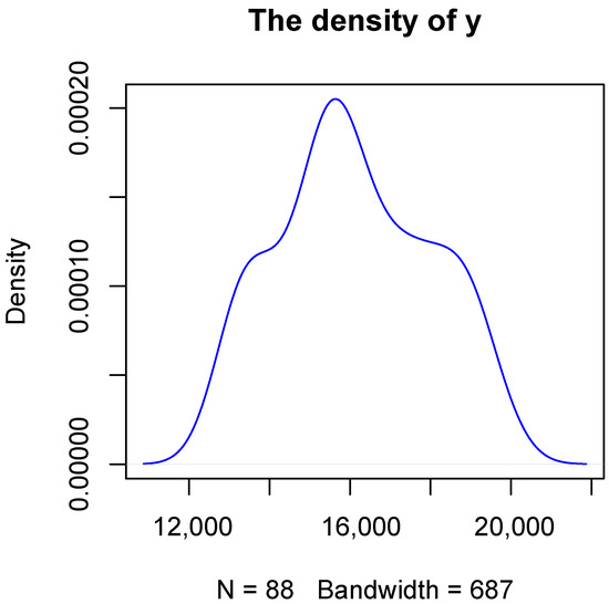
Figure 1. The density of the response.

The results are presented in Table 15. From the result, we can see that the model sizes of Farvsqr are 18, 19, 38, and 38 for the quantile $\tau =0.1,\tau =0.5,\tau =0.75,$ and $\tau =0.9$, respectively; however, the model sizes of LASSO are 241, 176, 207, and 222 for the quantile $\tau =0.1,\tau =0.5,\tau =0.75,$ and $\tau =0.9$, respectively. The LASSO prefers to choose more related variables. For instance, for $\tau =0.1,\tau =0.5,\tau =0.75,$ and $\tau =0.9$, all LASSO models include both Real PCE expenditures: durable goods, Real PCE: services, Real PCE: nondurable goods, Real gross private domestic investment, Real private fixed investment, Real gross private domestic investment: fixed investment: nonresidential: equipment, and Real private fixed investment: nonresidential because of the strong correlation between them. Moreover, all LASSO models also include both Number of civilians unemployed for less than 5 weeks, Number of civilians unemployed from 5 to 14 weeks, and Number of civilians unemployed from 15 to 26 weeks because of the strong correlation between them. Many other related variables are included by LASSO. The elapsed times of Farvsqr are 7.6209, 8.2036, 8.3589, and 8.3493 for the quantile $\tau =0.1,\tau =0.5,\tau =0.75,$ and $\tau =0.9$ respectively, while the elapsed times of LASSO are 9.8736, 13.8031, 10.6616, and 10.1012 for the quantile $\tau =0.1,\tau =0.5,\tau =0.75,$ and $\tau =0.9$, respectively; so we can say that the algorithm efficiency of LASSO for our real data is much lower than that of Farvsqr. It may be because LASSO selects too many redundant explanatory variables, which not only affects the estimation accuracy of the model but also affects the efficiency of the algorithm. For the $R^2$, Farvsqr is better than LASSO except for $\tau =0.1$. So, we can see that Farvsqr is more suitable for this data set. Furthermore, we can say that for the data set with strong correlation between explanatory variables, Farvsqr is more suitable for use.

Table 15. The results of the real data.

	${\mathit{R}}^2$		Model Size		Elapsed Time (Seconds)
$\mathit{\tau }$	Farvsqr	LASSO	Farvsqr	LASSO	Farvsqr	LASSO
$\tau =0.1$	0.9988	0.9993	18	241	7.6209	9.8736
$\tau =0.5$	0.9998	0.9996	19	176	8.2036	13.8031
$\tau =0.75$	0.9998	0.9995	38	207	8.3589	10.6616
$\tau =0.9$	0.9998	0.9993	38	222	8.3493	10.1012

7. Conclusions

In this paper, we are aimed at the data set, which has heavy-tailed distribution, high dimension, and high correlations within the blocks of the covariates. By generalizing the factor-adjusted regularized variable selection for mean regression to the quantile regression, we proposed the method of factor-augmented regularized variable selection for quantile regression ( Farvsqr). In order to analyze the theoretical analysis and improve estimation accuracy and computational efficiency for fitting large-scale linear quantile regression models, we use the convolution-type smoothed quantile regression to estimate the quantile regression coefficients. The paper gives the theoretical result of the estimators. At the same time, from the simulation and the real data analysis, we can see that our method is better than LASSO. In the future, we will continue to study the missing data variable selection for quantile regression with the high correlations within the blocks of the covariates.

Appendix A.1. Proof of Lemma 1

Let $\mathbf{V}={\left({\mathbf{v}}_1,\cdots ,{\mathbf{v}}_n\right)}^{\mathrm{T}}$ and ${\mathit{\theta }}^{*}={\left({\left({\mathit{\beta }}^{*}\right)}^{\mathrm{T}},{\left({\mathit{\beta }}^{*}\right)}^{\mathrm{T}}{\mathbf{\Lambda }}_0\right)}^{\mathrm{T}}$. Note that

$$\begin{array}{cc}\hfill & \nabla E\left[R\left(\mathbf{y},\mathbf{V}\mathit{\theta }\right)\right]=E\left\{\frac{1}{n}\sum _{i=1}^n[{\mathcal{K}}_h\left(\left(1,{\mathbf{x}}_i^{\mathrm{T}}\right)\mathit{\beta }-y_i\right)-\tau ]{\left(1,{\mathbf{x}}_i^{\mathrm{T}}\right)}^{\mathrm{T}}\right\}\hfill \\ \hfill & =E\left\{[{\mathcal{K}}_h\left(\left(1,{\mathbf{x}}_1^{\mathrm{T}}\right)\mathit{\beta }-y_1\right)-\tau ]{\left(1,{\mathbf{x}}_1^{\mathrm{T}}\right)}^{\mathrm{T}}\right\}\hfill \\ \hfill & =E\left\{[{\mathcal{K}}_h\left({\mathbf{v}}_1^{\mathrm{T}}\mathit{\theta }-y_1\right)-\tau ]{\mathbf{v}}_1\right\}\hfill \end{array}$$

and ${\mathbf{v}}_i^{\mathrm{T}}{\mathit{\theta }}^{*}=\left(1,{\mathbf{x}}_i^{\mathrm{T}}\right){\mathit{\beta }}^{*}$. So the conclusion can be proved by

$$\begin{array}{cc}\hfill & \nabla E\left[R\left(\mathbf{y},\mathbf{V}\mathit{\theta }\right)\right]{|}_{\mathit{\theta }={\mathit{\theta }}^{*}}\hfill \\ \hfill & =E\left\{[{\mathcal{K}}_h\left({\mathbf{v}}_1^{\mathrm{T}}{\mathit{\theta }}^{*}-y_1\right)-\tau ]{\mathbf{v}}_1\right\}\hfill \\ \hfill & =E\left\{[{\mathcal{K}}_h\left(\left(1,{\mathbf{x}}_1^{\mathrm{T}}\right){\mathit{\beta }}^{*}-y_1\right)-\tau ]{\mathbf{v}}_1\right\}\hfill \\ \hfill & =E\left[{\eta }_1{\mathbf{v}}_1\right]={\mathbf{0}}_{p+1+k}\hfill \end{array}$$

Appendix A.2. Proof of Theorem 1

In order to proof the theorem 1, let us introduce the Lemma A1 from Fan et al. [18] first. When we assume that the last k variables are not penalized, let $R(·):{\mathbb{R}}^{p+1+k}\to \mathbb{R}$ be a convex function, ${\mathit{\theta }}^{*}$ and ${\mathit{\beta }}^{*}={\mathit{\theta }}_{[p+1]}^{*}$ be the sparse sub-vector of interest. Then, ${\mathit{\theta }}^{*}$ and ${\mathit{\beta }}^{*}$ are estimated by

$$\begin{array}{cc}\hfill & \widehat{\mathit{\theta }}=argmin\{R\left(\mathit{\theta }\right)+\lambda \parallel {\mathit{\theta }}_{[p+1]}{\parallel }_1\}\hfill \\ \hfill & \widehat{\mathit{\beta }}={\widehat{\mathit{\theta }}}_{[p+1]}\hfill \end{array}$$

Let $L=supp\left({\mathit{\theta }}^{*}\right),L_1=supp\left({\mathit{\beta }}^{*}\right),L_2=[p+1+k]\backslash L$. Then, we can obtain the Lemma A1 as follows:

Assumption A1

(Smoothness). $R\left(\mathit{\theta }\right)\in C^2\left({\mathbb{R}}^{p+k+1}\right)$ and there exist $A>0,W>0$ such that $\parallel {\nabla }_{·L}^{2}R\left(\mathit{\theta }\right)-{\nabla }_{·L}^{2}R\left({\mathit{\theta }}^{*}\right){\parallel }_{\infty }\le W{\parallel \mathit{\theta }-{\mathit{\theta }}^{*}\parallel }_2$ whenever $supp\left(\mathit{\theta }\right)\in L$ and $\parallel \mathit{\theta }-{\mathit{\theta }}^{*}{\parallel }_2\le A$;

Assumption A2

(Restricted strong convexity). There exist ${\rho }_2>{\rho }_{\infty }>0$ such that $\parallel {\left[{\nabla }_{LL}^{2}R\left({\mathit{\theta }}^{*}\right)\right]}^{-1}{\parallel }_{\infty }\le \frac{1}{2{\rho }_{\infty }}$ and $\parallel {\left[{\nabla }_{LL}^{2}R\left({\mathit{\theta }}^{*}\right)\right]}^{-1}{\parallel }_2\le \frac{1}{2{\rho }_2}$;

Assumption A3

(Irrepresentable condition). $\parallel {\nabla }_{L_{2}L}^{2}R\left({\mathit{\theta }}^{*}\right){\left[{\nabla }_{LL}^{2}R\left({\mathit{\theta }}^{*}\right)\right]}^{-1}{\parallel }_{\infty }\le 1-\gamma$ for some $\gamma \in (0,1)$;

Lemma A1.

Under Assumptions A1–A3, if

$$\frac{7}{\gamma }{\parallel \nabla R\left({\mathit{\theta }}^{*}\right)\parallel }_{\infty }<\lambda <\frac{{\rho }_2}{4L}minA,\frac{{\rho }_{\infty }\gamma }{3W}$$

then $supp\left(\widehat{\mathit{\theta }}\right)\subset L$ and

$$\begin{array}{cc}\hfill & \parallel \widehat{\mathit{\theta }}-{\mathit{\theta }}^{*}{\parallel }_{\infty }\le \frac{3}{5{\rho }_{\infty }}\left(\parallel {\nabla }_{L}R\left({\mathit{\theta }}^{*}\right){\parallel }_{\infty }+\lambda \right)\hfill \\ \hfill & \parallel \widehat{\mathit{\theta }}-{\mathit{\theta }}^{*}{\parallel }_2\le \frac{2}{{\rho }_2}\left(\parallel {\nabla }_{L}R\left({\mathit{\theta }}^{*}\right){\parallel }_2+\lambda \sqrt{L_1}\right)\hfill \\ \hfill & \parallel \widehat{\mathit{\theta }}-{\mathit{\theta }}^{*}{\parallel }_1\le min\frac{3}{5{\rho }_{\infty }}\left(\parallel {\nabla }_{L}R\left({\mathit{\theta }}^{*}\right){\parallel }_1+\lambda \sqrt{L_1}\right),\frac{2\sqrt{L}}{{\rho }_2}\left(\parallel {\nabla }_{L}R\left({\mathit{\theta }}^{*}\right){\parallel }_2+\lambda \sqrt{L_1}\right).\hfill \end{array}$$

Next, we will give the proof of the Theorem 1.

Proof of Theorem 1.

As we know, $\widehat{\mathit{\theta }}=argmi{n}_{\mathit{\theta }}\{R(\mathbf{y},\widehat{\mathbf{V}}\mathit{\theta })+\lambda \parallel {\mathit{\theta }}_{[p+1]}{\parallel }_1\}$. From Assumption 4, we know that ${\mathbf{M}}_0$ is nonsingular and $\mathbf{M}=\left(\begin{array}{cc}{\mathbf{I}}_{p+1}& {\mathbf{0}}_{(p+1)\times k}\\ {\mathbf{0}}_{(p+1)\times k}& {\mathbf{M}}_0\end{array}\right)$. Let $\overline{\mathbf{V}}=\widehat{\mathbf{V}}\mathbf{M},\overline{\mathit{\theta }}={\mathbf{M}}^{-1}\widehat{\mathit{\theta }},{\widehat{\mathbf{\Lambda }}}_0={\left({\mathbf{0}}_k^{\mathrm{T}},{\widehat{\mathbf{\Lambda }}}^{\mathrm{T}}\right)}^{\mathrm{T}},{\widehat{\mathit{\theta }}}^{*}=\left(\begin{array}{c}{\mathit{\beta }}^{*}\\ {\widehat{\mathbf{\Lambda }}}_0{\mathit{\beta }}^{*}\end{array}\right),{\overline{\mathit{\theta }}}^{*}={\mathbf{M}}^{-1}{\widehat{\mathit{\theta }}}^{*}$. So, we can see that $\widehat{\mathit{\beta }}={\widehat{\mathit{\theta }}}_{[p+1]}={\overline{\mathit{\theta }}}_{[p+1]}$ and $\overline{\mathit{\theta }}=argmi{n}_{\mathit{\theta }}\{R(\mathbf{y},\overline{\mathbf{V}}\mathit{\theta })+\lambda \parallel {\mathit{\theta }}_{[p+1]}{\parallel }_1\}$. So, $supp\left(\widehat{\mathit{\beta }}\right)=supp\left({\overline{\mathit{\theta }}}_{[p+1]}\right)$ and $\parallel \widehat{\mathit{\beta }}-{\mathit{\beta }}^{*}\parallel =\parallel {\overline{\mathit{\theta }}}_{[p+1]}-{\overline{\mathit{\theta }}}_{[p+1]}^{*}\parallel \le \parallel \overline{\mathit{\theta }}-{\overline{\mathit{\theta }}}^{*}\parallel$ for any norm.

Then, we can change to study $\overline{\mathit{\theta }}$ and the objective function $R\left(\mathbf{y},\overline{\mathbf{V}}\mathit{\theta }\right)$ in order to study the theoretical properties of $\widehat{\mathit{\beta }}$. We will give the Theorem A1 which means all the assumptions in Lemma A1 are fulfilled.

Let ${\mathbf{v}}_i^{\mathrm{T}}$ and ${\overline{\mathbf{v}}}_i^{\mathrm{T}}$ be the $i-$th row of $\mathbf{V}$ and $\overline{\mathbf{V}}$, respectively. We can see that $R\left(\mathbf{y},\overline{\mathbf{V}}\mathit{\theta }\right)=\frac{1}{n}{\sum }_{i=1}^n{\mathcal{L}}_h(y_i-{\overline{\mathbf{v}}}_i^{\mathrm{T}}\mathit{\theta }),\nabla R\left(\mathbf{y},\overline{\mathbf{V}}\mathit{\theta }\right)=\frac{1}{n}{\sum }_{i=1}^n\{{\mathcal{K}}_h\left({\overline{\mathbf{v}}}_i^{\mathrm{T}}\mathit{\theta }-y_i\right)-\tau \}{\overline{\mathbf{v}}}_i$, $\overline{\mathbf{V}}{\overline{\mathit{\theta }}}^{*}=\mathbf{X}{\mathit{\beta }}^{*}$. Hence $\parallel \nabla R\left(\mathbf{y},\overline{\mathbf{V}}{\overline{\mathit{\theta }}}^{*}\right){\parallel }_{\infty }=\omega$. From the properties of the vector norm, we can obtain $\parallel {\nabla }_{L}R\left(\mathbf{y},\overline{\mathbf{V}}{\overline{\mathit{\theta }}}^{*}\right){\parallel }_{\infty }\le \omega ,\parallel {\nabla }_{L}R\left(\mathbf{y},\overline{\mathbf{V}}{\overline{\mathit{\theta }}}^{*}\right){\parallel }_2\le \omega \sqrt{L},{\parallel {\nabla }_{L}R\left(\mathbf{y},\overline{\mathbf{V}}{\overline{\mathit{\theta }}}^{*}\right)\parallel }_1\le \omega L$. In addition, let $\lambda >\frac{7\omega }{\gamma }\ge \omega$. From Lemma A1, we can obtain that Theorem 1 is true.  □

Theorem A1.

Based on all the Assumptions 2–4, define $W=W_0^3{W}_3{L}^{3/2}$, then

$$\begin{array}{cc}\hfill & \left(i\right)\parallel {\nabla }_{·L}^{2}R\left(\mathbf{y},\overline{\mathbf{V}}\mathit{\theta }\right)-{\nabla }_{·L}^{2}R\left(\mathbf{y},\overline{\mathbf{V}}{\overline{\mathit{\theta }}}^{*}\right){\parallel }_{\infty }\le W{\parallel \mathit{\theta }-{\overline{\mathit{\theta }}}^{*}\parallel }_2,\hfill \\ \hfill & \left(ii\right)\parallel {\left[{\nabla }_{LL}^{2}R\left(\mathbf{y},\overline{\mathbf{V}}{\overline{\mathit{\theta }}}^{*}\right)\right]}^{-1}{\parallel }_{\infty }\le \frac{1}{2{\rho }_{\infty }},\hfill \\ \hfill & \left(iii\right)\parallel {\left[{\nabla }_{LL}^{2}R\left(\mathbf{y},\overline{\mathbf{V}}{\overline{\mathit{\theta }}}^{*}\right)\right]}^{-1}{\parallel }_2\le \frac{1}{2{\rho }_2},\hfill \\ \hfill & \left(iv\right)\parallel {\nabla }_{L_{2}L}^{2}R\left(\mathbf{y},\overline{\mathbf{V}}{\overline{\mathit{\theta }}}^{*}\right){\left[{\nabla }_{LL}^{2}R\left(\mathbf{y},\overline{\mathbf{V}}{\overline{\mathit{\theta }}}^{*}\right)\right]}^{-1}{\parallel }_{\infty }\le 1-\gamma .\hfill \end{array}$$

Proof. 

(i) $\mathbf{V}{\mathit{\theta }}^{*}=\overline{\mathbf{V}}{\overline{\mathit{\theta }}}^{*}=\mathbf{X}{\mathit{\beta }}^{*}$, then

$$\begin{array}{cc}\hfill & {\nabla }^{2}R\left(\mathbf{y},\mathbf{V}{\mathit{\theta }}^{*}\right)=\frac{1}{n}\sum _{i=1}^n\left\{K_h\left({\overline{\mathbf{v}}}_i^{\mathrm{T}}{\overline{\mathit{\theta }}}^{*}-y_i\right)\right\}{\mathbf{v}}_i{\mathbf{v}}_i^{\mathrm{T}},\hfill \\ \hfill & {\nabla }^{2}R\left(\mathbf{y},\overline{\mathbf{V}}{\overline{\mathit{\theta }}}^{*}\right)=\frac{1}{n}\sum _{i=1}^n\left\{K_h\left({\overline{\mathbf{v}}}_i^{\mathrm{T}}{\overline{\mathit{\theta }}}^{*}-y_i\right)\right\}{\overline{\mathbf{v}}}_i{\overline{\mathbf{v}}}_i^{\mathrm{T}}.\hfill \end{array}$$

For any $j,t\in [p+1+k]$ and $supp\left(\mathit{\theta }\right)\in L$, we have

$$\begin{array}{cc}\hfill & \left|{\nabla }_{jt}^{2}R\left(\mathbf{y},\overline{\mathbf{V}}\mathit{\theta }\right)-{\nabla }_{jt}^{2}R\left(\mathbf{y},\overline{\mathbf{V}}{\overline{\mathit{\theta }}}^{*}\right)\right|\hfill \\ \hfill & =\frac{1}{n}\left|\sum _{i=1}^n{K}_h\left({\overline{\mathbf{v}}}_i^{\mathrm{T}}\mathit{\theta }-y_i\right){\overline{v}}_{ij}{\overline{v}}_{it}-\sum _{i=1}^n{K}_h\left({\overline{\mathbf{v}}}_i^{\mathrm{T}}{\overline{\mathit{\theta }}}^{*}-y_i\right){\overline{v}}_{ij}{\overline{v}}_{it}\right|\hfill \\ \hfill & =\frac{1}{n}\left|\sum _{i=1}^n[K_h\left({\overline{\mathbf{v}}}_i^{\mathrm{T}}\mathit{\theta }-y_i\right)-K_h\left({\overline{\mathbf{v}}}_i^{\mathrm{T}}{\overline{\mathit{\theta }}}^{*}-y_i\right)]{\overline{v}}_{ij}{\overline{v}}_{it}\right|\hfill \\ \hfill & \le \frac{1}{n}\sum _{i=1}^n\left|K_h\left({\overline{\mathbf{v}}}_i^{\mathrm{T}}\mathit{\theta }-y_i\right)-K_h\left({\overline{\mathbf{v}}}_i^{\mathrm{T}}{\overline{\mathit{\theta }}}^{*}-y_i\right)\right|\left|{\overline{v}}_{ij}{\overline{v}}_{it}\right|\hfill \\ \hfill & \le \frac{1}{n}\sum _{i=1}^n{W}_3\left|{\mathbf{v}}_i^{\mathrm{T}}\left(\mathit{\theta }-{\mathit{\theta }}^{*}\right)\right|{\parallel \overline{\mathbf{V}}\parallel }_{max}^2\hfill \end{array}$$

(A1)

By the Cauchy–Schwarz inequality and $\parallel \overline{\mathbf{V}}{\parallel }_{max}\le {\parallel \mathbf{V}\parallel }_{max}+{\parallel \overline{\mathbf{V}}-\mathbf{V}\parallel }_{max}\le W_0$, so for $i\in \left[n\right]$, we have $\left|{\overline{\mathbf{v}}}_i^{\mathrm{T}}\left(\mathit{\theta }-{\overline{\mathit{\theta }}}^{*}\right)\right|=\left|{\overline{\mathbf{v}}}_{iL}^{\mathrm{T}}{\left(\mathit{\theta }-{\overline{\mathit{\theta }}}^{*}\right)}_L\right|\le \parallel {\overline{\mathbf{v}}}_{iL}{\parallel }_2\parallel \mathit{\theta }-{\overline{\mathit{\theta }}}^{*}{\parallel }_2\le \sqrt{L}{W}_0{\parallel \mathit{\theta }-{\overline{\mathit{\theta }}}^{*}\parallel }_2$. Plugging this result back to (A1), we can obtain

$$\begin{array}{cc}\hfill & \left|{\nabla }_{jt}^{2}R\left(\mathbf{y},\overline{\mathbf{V}}\mathit{\theta }\right)-{\nabla }_{jt}^{2}R\left(\mathbf{y},\overline{\mathbf{V}}{\overline{\mathit{\theta }}}^{*}\right)\right|\le \sqrt{L}{W}_3{W}_0^3{\parallel \mathit{\theta }-{\overline{\mathit{\theta }}}^{*}\parallel }_2,\forall j,t\in [p+1+k]\hfill \\ \hfill & \parallel {\nabla }_{·L}^{2}R\left(\mathbf{y},\overline{\mathbf{V}}\mathit{\theta }\right)-{\nabla }_{·L}^{2}R\left(\mathbf{y},\overline{\mathbf{V}}{\overline{\mathit{\theta }}}^{*}\right){\parallel }_{\infty }\le L^{3/2}{W}_3{W}_0^3\parallel \mathit{\theta }-{\overline{\mathit{\theta }}}^{*}{{\parallel }_2=M\mathit{\theta }-{\overline{\mathit{\theta }}}^{*}\parallel }_2.\hfill \end{array}$$

(ii) For any $t\in [p+1+k]$, we have

$$\begin{array}{cc}\hfill & \parallel {\nabla }_{tL}^{2}R\left(\mathbf{y},\overline{\mathbf{V}}{\overline{\mathit{\theta }}}^{*}\right)-{\nabla }_{·L}^{2}R\left(\mathbf{y},\mathbf{V}{\mathit{\theta }}^{*}\right){\parallel }_{\infty }=\frac{1}{n}{\parallel \sum _{i=1}^n{K}_h({\overline{\mathbf{v}}}_i^{\mathrm{T}}{\overline{\mathit{\theta }}}^{*}-y_i)({\overline{v}}_{it}{\overline{\mathbf{v}}}_{iL}^{\mathrm{T}}-v_{it}{\mathbf{v}}_{iL}^{\mathrm{T}})\parallel }_{\infty }\hfill \\ \hfill & \le \frac{1}{n}\sum _{i=1}^n{K}_h({\overline{\mathbf{v}}}_i^{\mathrm{T}}{\overline{\mathit{\theta }}}^{*}-y_i)\parallel {\overline{v}}_{it}{\overline{\mathbf{v}}}_{iL}^{\mathrm{T}}-v_{it}{\mathbf{v}}_{iL}^{\mathrm{T}}{\parallel }_{max}\le \frac{W_2\sqrt{L}}{n}\sum _{i=1}^n{\parallel {\overline{v}}_{it}{\overline{\mathbf{v}}}_{iL}^{\mathrm{T}}-v_{it}{\mathbf{v}}_{iL}^{\mathrm{T}}\parallel }_2.\hfill \end{array}$$

With ${\parallel \mathbf{V}\parallel }_{max}\le W_0/2,{\parallel \overline{\mathbf{V}}\parallel }_{max}\le W_0$, we can obtain

$$\begin{array}{cc}\hfill & \parallel {\overline{v}}_{it}{\overline{\mathbf{v}}}_{iL}^{\mathrm{T}}-v_{it}{\mathbf{v}}_{iL}^{\mathrm{T}}{\parallel }_2={\parallel {\overline{v}}_{it}{\overline{\mathbf{v}}}_{iL}^{\mathrm{T}}-v_{it}{\mathbf{v}}_{iL}^{\mathrm{T}}+v_{it}{\overline{\mathbf{v}}}_{iL}^{\mathrm{T}}-v_{it}{\overline{\mathbf{v}}}_{iL}^{\mathrm{T}}\parallel }_2\hfill \\ \hfill & \le \parallel v_{it}{({\overline{\mathbf{v}}}_{iL}-{\mathbf{v}}_{iL})}^{\mathrm{T}}{\parallel }_2+{\parallel ({\overline{v}}_{it}-v_{it}){\overline{\mathbf{v}}}_{iL}^{\mathrm{T}}\parallel }_2\hfill \\ \hfill & \le \left|v_{it}\right|\parallel {\overline{\mathbf{v}}}_{iL}-{\mathbf{v}}_{iL}{\parallel }_2+\left|{\overline{v}}_{it}-v_{it}\right|{\parallel {\overline{\mathbf{v}}}_{iL}^{\mathrm{T}}\parallel }_2\hfill \\ \hfill & \le {\parallel \mathbf{V}\parallel }_{max}\parallel {\overline{\mathbf{v}}}_{iL}-{\mathbf{v}}_{iL}{\parallel }_2+\left|{\overline{v}}_{it}-v_{it}\right|\sqrt{L}{\parallel \overline{\mathbf{V}}\parallel }_{max}\hfill \\ \hfill & \le \frac{W_0}{2}{\parallel {\overline{\mathbf{v}}}_{iL}-{\mathbf{v}}_{iL}\parallel }_2+W_0\sqrt{L}\left|{\overline{v}}_{it}-v_{it}\right|.\hfill \end{array}$$

From Assumption 4, we know that $\sigma =ma{x}_{j\in [p+1+k]}{\left(\frac{1}{n}{\sum }_{i=1}^n{\left|{\overline{v}}_{ij}-v_{ij}\right|}^2\right)}^{1/2}$. By Jensen’s inequality, $\forall J\subseteq [p+1+k]$, we have

$$\begin{array}{cc}\hfill & \frac{1}{n}\sum _{i=1}^n{\parallel {\overline{\mathbf{v}}}_{iJ}-{\mathbf{v}}_{iJ}\parallel }_2\le {\left(\frac{1}{n}\sum _{i=1}^n{\parallel {\overline{\mathbf{v}}}_{iJ}-{\mathbf{v}}_{iJ}\parallel }_2^2\right)}^{1/2}\hfill \\ \hfill & \le {\left(\frac{J}{n}ma{x}_{j\in [p+1+k]{\sum }_{i=1}^n}\left|{\overline{v}}_{ij}-v_{ij}\right|\right)}^{1/2}\le \sqrt{L}\sigma .\hfill \end{array}$$

So

$$\begin{array}{cc}\hfill & \parallel {\nabla }_{·L}^{2}R\left(\mathbf{y},\overline{\mathbf{V}}{\mathit{\theta }}^{*}\right)-{\nabla }_{·L}^{2}R\left(\mathbf{y},\mathbf{V}{\mathit{\theta }}^{*}\right){\parallel }_{\infty }\hfill \\ \hfill & =L·ma{x}_{j\in [p+1+k]}{\parallel {\nabla }_{jL}^{2}R\left(\mathbf{y},\overline{\mathbf{V}}{\mathit{\theta }}^{*}\right)-{\nabla }_{jL}^{2}R\left(\mathbf{y},\mathbf{V}{\mathit{\theta }}^{*}\right)\parallel }_{\infty }\hfill \\ \hfill & \le L\frac{W_2\sqrt{L}}{N}\sum _{i=1}^n\left(\frac{W_0}{2}{\parallel {\overline{\mathbf{v}}}_{iL}-{\mathbf{v}}_{iL}\parallel }_2+W_0\sqrt{L}\left|{\overline{v}}_{ij}-v_{ij}\right|\right)\hfill \\ \hfill & =\frac{W_0{W}_2\sqrt{L}}{2}\frac{1}{n}\sum _{i=1}^n{\parallel {\overline{\mathbf{v}}}_{iL}-{\mathbf{v}}_{iL}\parallel }_2+W_0{W}_2{L}^2\frac{1}{n}\sum _{i=1}^n\left|{\overline{v}}_{ij}-v_{ij}\right|\hfill \\ \hfill & \le \frac{W_0{W}_2{L}^2}{2}\sigma +W_0{W}_2{L}^2\sigma \hfill \\ \hfill & =\frac{3}{2}{W}_0{W}_2{L}^2\sigma .\hfill \end{array}$$

(A2)

Let $\kappa =\parallel {\left({\nabla }_{LL}^{2}R\left(\mathbf{y},\mathbf{V}{\mathit{\theta }}^{*}\right)\right)}^{-1}[{\nabla }_{LL}^{2}R\left(\mathbf{y},\overline{\mathbf{V}}{\overline{\mathit{\theta }}}^{*}\right)-{\nabla }_{LL}^{2}R\left(\mathbf{y},\mathbf{V}{\mathit{\theta }}^{*}\right)]{\parallel }_{\infty }$, then we can obtain

$$\begin{array}{cc}\hfill & \kappa \le \parallel {\left({\nabla }_{LL}^{2}R\left(\mathbf{y},\mathbf{V}{\mathit{\theta }}^{*}\right)\right)}^{-1}{\parallel }_{\infty }{\parallel {\nabla }_{LL}^{2}R\left(\mathbf{y},\overline{\mathbf{V}}{\overline{\mathit{\theta }}}^{*}\right)-{\nabla }_{LL}^{2}R\left(\mathbf{y},\mathbf{V}{\mathit{\theta }}^{*}\right)\parallel }_{\infty }\hfill \\ \hfill & \le \frac{3}{8{\rho }_{\infty }}{W}_0{W}_2{L}^2\sigma \hfill \\ \hfill & \le \frac{1}{2}\hfill \end{array}$$

(A3)

And

$$\begin{array}{cc}\hfill & \parallel {\left({\nabla }_{LL}^{2}R\left(\mathbf{y},\overline{\mathbf{V}}{\overline{\mathit{\theta }}}^{*}\right)\right)}^{-1}-{\left({\nabla }_{LL}^{2}R\left(\mathbf{y},\mathbf{V}{\mathit{\theta }}^{*}\right)\right)}^{-1}{\parallel }_{\infty }\hfill \\ \hfill & \le \parallel {\left({\nabla }_{LL}^{2}R\left(\mathbf{y},\mathbf{V}{\mathit{\theta }}^{*}\right)\right)}^{-1}{\parallel }_{\infty }\frac{\kappa }{1-\kappa }\hfill \\ \hfill & \le \frac{1}{4{\rho }_{\infty }}\hfill \end{array}$$

So

$$\begin{array}{cc}\hfill & \parallel {\left({\nabla }_{LL}^{2}R\left(\mathbf{y},\overline{\mathbf{V}}{\overline{\mathit{\theta }}}^{*}\right)\right)}^{-1}{\parallel }_{\infty }\hfill \\ \hfill & \le \parallel {\left({\nabla }_{LL}^{2}R\left(\mathbf{y},\mathbf{V}{\mathit{\theta }}^{*}\right)\right)}^{-1}{\parallel }_{\infty }+\frac{1}{4{\rho }_{\infty }}\hfill \\ \hfill & \frac{1}{2{\rho }_{\infty }}\hfill \end{array}$$

(A4)

(iii) The third conclusion can be obtained easily from (A4). Since for any symmetric matrix B, ${\parallel B\parallel }_2\le {\parallel B\parallel }_{\infty }$ is satisfied. We can obtain $\parallel {\left({\nabla }_{LL}^{2}R\left(\mathbf{y},\overline{\mathbf{V}}{\overline{\mathit{\theta }}}^{*}\right)\right)}^{-1}-{\left({\nabla }_{LL}^{2}R\left(\mathbf{y},\mathbf{V}{\mathit{\theta }}^{*}\right)\right)}^{-1}{\parallel }_2\le \frac{1}{4{\rho }_{\infty }}\le \frac{1}{4{\rho }_2}$, and thus

$$\parallel {\left({\nabla }_{LL}^{2}R\left(\mathbf{y},\overline{\mathbf{V}}{\overline{\mathit{\theta }}}^{*}\right)\right)}^{-1}{\parallel }_2\le \frac{1}{2{\rho }_2}$$

(iv)

$$\begin{array}{cc}\hfill & \parallel {\nabla }_{L_{2}L}^{2}R\left(\mathbf{y},\overline{\mathbf{V}}{\overline{\mathit{\theta }}}^{*}\right){\left({\nabla }_{LL}^{2}R\left(\mathbf{y},\overline{\mathbf{V}}{\overline{\mathit{\theta }}}^{*}\right)\right)}^{-1}-{\nabla }_{L_{2}L}^{2}R\left(\mathbf{y},\mathbf{V}{\mathit{\theta }}^{*}\right){\left({\nabla }_{LL}^{2}R\left(\mathbf{y},\mathbf{V}{\mathit{\theta }}^{*}\right)\right)}^{-1}{\parallel }_{\infty }\hfill \\ \hfill & =\parallel {\nabla }_{L_{2}L}^{2}R\left(\mathbf{y},\overline{\mathbf{V}}{\overline{\mathit{\theta }}}^{*}\right){\left({\nabla }_{LL}^{2}R\left(\mathbf{y},\overline{\mathbf{V}}{\overline{\mathit{\theta }}}^{*}\right)\right)}^{-1}+{\nabla }_{L_{2}L}^{2}R\left(\mathbf{y},\mathbf{V}{\mathit{\theta }}^{*}\right){\left({\nabla }_{LL}^{2}R\left(\mathbf{y},\overline{\mathbf{V}}{\overline{\mathit{\theta }}}^{*}\right)\right)}^{-1}\hfill \\ \hfill & -{\nabla }_{L_{2}L}^{2}R\left(\mathbf{y},\mathbf{V}{\mathit{\theta }}^{*}\right){\left({\nabla }_{LL}^{2}R\left(\mathbf{y},\overline{\mathbf{V}}{\overline{\mathit{\theta }}}^{*}\right)\right)}^{-1}-{\nabla }_{L_{2}L}^{2}R\left(\mathbf{y},\mathbf{V}{\mathit{\theta }}^{*}\right){\left({\nabla }_{LL}^{2}R\left(\mathbf{y},\mathbf{V}{\mathit{\theta }}^{*}\right)\right)}^{-1}{\parallel }_{\infty }\hfill \\ \hfill & \le \parallel {\nabla }_{L_{2}L}^{2}R\left(\mathbf{y},\overline{\mathbf{V}}{\overline{\mathit{\theta }}}^{*}\right)-{\nabla }_{L_{2}L}^{2}R\left(\mathbf{y},\mathbf{V}{\mathit{\theta }}^{*}\right){\parallel }_{\infty }{\parallel {\left({\nabla }_{LL}^{2}R\left(\mathbf{y},\overline{\mathbf{V}}{\overline{\mathit{\theta }}}^{*}\right)\right)}^{-1}\parallel }_{\infty }\hfill \\ \hfill & +\parallel {\nabla }_{L_{2}L}^{2}R\left(\mathbf{y},\mathbf{V}{\mathit{\theta }}^{*}\right)[{\left({\nabla }_{LL}^{2}R\left(\mathbf{y},\overline{\mathbf{V}}{\overline{\mathit{\theta }}}^{*}\right)\right)}^{-1}-{\left({\nabla }_{LL}^{2}R\left(\mathbf{y},\mathbf{V}{\mathit{\theta }}^{*}\right)\right)}^{-1}]{\parallel }_{\infty }\hfill \end{array}$$

From the conclusion (ii) and (A2), we can obtain that

$$\parallel {\nabla }_{L_{2}L}^{2}R\left(\mathbf{y},\overline{\mathbf{V}}{\overline{\mathit{\theta }}}^{*}\right)-{\nabla }_{L_{2}L}^{2}R\left(\mathbf{y},\mathbf{V}{\mathit{\theta }}^{*}\right){\parallel }_{\infty }{\parallel {\left({\nabla }_{LL}^{2}R\left(\mathbf{y},\overline{\mathbf{V}}{\overline{\mathit{\theta }}}^{*}\right)\right)}^{-1}\parallel }_{\infty }\le \frac{3}{4{\rho }_{\infty }}{W}_0{W}_2{L}^2\sigma$$

On the other hand, we can take $A={\nabla }_{L_{2}L}^{2}R\left(\mathbf{y},\mathbf{V}{\mathit{\theta }}^{*}\right),B={\nabla }_{LL}^{2}R\left(\mathbf{y},\mathbf{V}{\mathit{\theta }}^{*}\right),C={\nabla }_{LL}^{2}R\left(\mathbf{y},\overline{\mathbf{V}}{\overline{\mathit{\theta }}}^{*}\right)-{\nabla }_{LL}^{2}R\left(\mathbf{y},\mathbf{V}{\mathit{\theta }}^{*}\right)$. By Assumption 4, $\parallel A{B}^{-1}{\parallel }_{\infty }\le 1-2\gamma \le 1$, and we have

$$\begin{array}{cc}\hfill & \parallel {\nabla }_{L_{2}L}^{2}R\left(\mathbf{y},\mathbf{V}{\mathit{\theta }}^{*}\right){[{\left({\nabla }_{LL}^{2}R\left(\mathbf{y},\overline{\mathbf{V}}{\overline{\mathit{\theta }}}^{*}\right)\right)}^{-1}-{\left({\nabla }_{LL}^{2}R\left(\mathbf{y},\mathbf{V}{\mathit{\theta }}^{*}\right)\right)}^{-1}\parallel }_{\infty }\hfill \\ \hfill & =\parallel A[{(B+C)}^{-1}-B^{-1}]{\parallel }_{\infty }\hfill \\ \hfill & \le \parallel A{B}^{-1}{\parallel }_{\infty }\frac{\parallel C{B}^{-1}{\parallel }_{\infty }}{1-\parallel C{B}^{-1}{\parallel }_{\infty }}\hfill \\ \hfill & \le \frac{{\parallel C\parallel }_{\infty }{\parallel B^{-1}\parallel }_{\infty }}{1-{\parallel C\parallel }_{\infty }{\parallel B^{-1}\parallel }_{\infty }}\hfill \end{array}$$

From Formula (A3), we can obtain ${\parallel C\parallel }_{\infty }{\parallel B^{-1}\parallel }_{\infty }\le \frac{3}{8{\rho }_{\infty }}{W}_0{W}_2{L}^2\sigma \le \frac{1}{2}$. As a result,

$$\parallel {\nabla }_{L_{2}L}^{2}R\left(\mathbf{y},\mathbf{V}{\mathit{\theta }}^{*}\right){[{\left({\nabla }_{LL}^{2}R\left(\mathbf{y},\overline{\mathbf{V}}{\overline{\mathit{\theta }}}^{*}\right)\right)}^{-1}-{\left({\nabla }_{LL}^{2}R\left(\mathbf{y},\mathbf{V}{\mathit{\theta }}^{*}\right)\right)}^{-1}\parallel }_{\infty }\le \frac{3}{4{\rho }_{\infty }}{W}_0{W}_2{L}^2\sigma$$

By combining these estimates, we have

$$\begin{array}{cc}\hfill & \parallel {\nabla }_{L_{2}L}^{2}R\left(\mathbf{y},\overline{\mathbf{V}}{\overline{\mathit{\theta }}}^{*}\right){\left({\nabla }_{LL}^{2}R\left(\mathbf{y},\overline{\mathbf{V}}{\overline{\mathit{\theta }}}^{*}\right)\right)}^{-1}-{\nabla }_{L_{2}L}^{2}R\left(\mathbf{y},\mathbf{V}{\mathit{\theta }}^{*}\right){\left({\nabla }_{LL}^{2}R\left(\mathbf{y},\mathbf{V}{\mathit{\theta }}^{*}\right)\right)}^{-1}{\parallel }_{\infty }\hfill \\ \hfill & \le \frac{3}{4{\rho }_{\infty }}{W}_0{W}_2{L}^2\sigma +\frac{3}{4{\rho }_{\infty }}{W}_0{W}_2{L}^2\sigma \hfill \\ \hfill & \le \frac{3}{2{\rho }_{\infty }}{W}_0{W}_2{L}^2\sigma \hfill \\ \hfill & \le \gamma \hfill \end{array}$$

Therefore, $\parallel {\nabla }_{L_{2}L}^{2}R\left(\mathbf{y},\overline{\mathbf{V}}{\overline{\mathit{\theta }}}^{*}\right){\left({\nabla }_{LL}^{2}R\left(\mathbf{y},\overline{\mathbf{V}}{\overline{\mathit{\theta }}}^{*}\right)\right)}^{-1}{\parallel }_{\infty }\le (1-2\gamma )+\gamma =1-\gamma$.  □

References

- Tibshirani, R. Regression shrinkage and selection via the lasso. J. R. Stat. Soc. Ser. B Stat. Methodol. 1996, 58, 267–288. [Google Scholar] [CrossRef]
- Fan, J.; Li, R. Variable selection via nonconcave penalized likelihood and its oracle properties. J. Am. Stat. Assoc. 2001, 96, 1348–1360. [Google Scholar] [CrossRef]
- Zou, H.; Hastie, T. Regularization and variable selection via the elastic net. J. R. Stat. Soc. Ser. B Stat. Methodol. 2005, 67, 301–320. [Google Scholar] [CrossRef]
- Candes, E.; Tao, T. The Dantzig selector: Statistical estimation when p is much larger than n. Ann. Stat. 2007, 35, 2313–2351. [Google Scholar]
- Donoho, D.L.; Elad, M. Optimally sparse representation in general (nonorthogonal) dictionaries via l1 minimization. Proc. Natl. Acad. Sci. USA 2003, 100, 2197–2202. [Google Scholar] [CrossRef]
- Fan, J.; Peng, H. On non-concave penalized likelihood with diverging number of parameters. Ann. Stat. 2004, 32, 928–961. [Google Scholar] [CrossRef]
- Efron, B.; Hastie, T.; Johnstone, I.; Tibshirani, R. Least angle regression. Ann. Stat. 2004, 32, 407–499. [Google Scholar] [CrossRef]
- Meinshausen, N.; Bühlmann, P. High-dimensional graphs and variable selection with the lasso. Ann. Stat. 2006, 34, 1436–1462. [Google Scholar] [CrossRef]
- Zhao, P.L.; Yu, B. On model selection consistency of Lasso. J. Mach. Learn. Res. 2006, 7, 2541–2563. [Google Scholar]
- Fan, J.; Lv, J. Sure independence screening for ultrahigh dimensional feature space. J. R. Stat. Soc. Ser. B Stat. Methodol. 2008, 70, 849–911. [Google Scholar] [CrossRef] [PubMed]
- Zou, H.; Li, R. One-step sparse estimates in nonconcave penalized likelihood models. Ann. Stat. 2008, 36, 1509–1533. [Google Scholar]
- Bickel, P.J.; Ritov, Y.A.; Tsybakov, A.B. Simultaneous analysis of lasso and dantzig selector. Ann. Stat. 2009, 37, 1705–1732. [Google Scholar] [CrossRef]
- Wainwright, M.J. Sharp thresholds for high-dimensional and noisy sparsity recovery using-constrained quadratic programming (lasso) quadratic programming (Lasso). IEEE Trans. Inform. Theory 2009, 55, 2183–2202. [Google Scholar] [CrossRef]
- Zhang, C.H. Nearly unbiased variable selection under minimax concave penalty. Ann. Stat. 2010, 38, 894–942. [Google Scholar] [CrossRef]
- Stock, J.; Watson, M. Forecasting using principal components from a large number of predictors. J. Am. Stat. Assoc. 2002, 97, 1167–1179. [Google Scholar] [CrossRef]
- Bai, J.; Ng, S. Determining the number of factors in approximate factor models. Econometrica 2002, 70, 191–221. [Google Scholar] [CrossRef]
- McCracken, M.; Ng, S. FRED-QD: A Quarterly Database for Macroeconomic Research; Federal Reserve Bank of St. Louis: St. Louis, MO, USA, 2021. [Google Scholar]
- Fan, J.; Ke, Y.; Wang, K. Factor-Adjusted Regularized Model Selection. J. Econom. 2020, 216, 71–85. [Google Scholar] [CrossRef]
- Koenker, R.; Bassett, G. Regression quantiles. Econometrica 1978, 46, 33–50. [Google Scholar] [CrossRef]
- Koenker, R. Quantile Regression; Cambridge University Press: Cambridge, UK, 2005. [Google Scholar]
- Koenker, R.; Chernozhukov, V.; He, X.; Peng, L. Handbook of Quantile Regression; CRC Press: New York, NY, USA, 2017. [Google Scholar]
- Ando, T.; Tsay, R.S. Quantile regression models with factor-augmented predictors and information criterion. Econom. J. 2011, 14, 1–24. [Google Scholar] [CrossRef]
- Hirzel, A.H.; Hausser, J.; Chessel, D.; Perrin, N. Ecological-niche factor analysis: How to compute habitat-suitability maps without absence data? Ecology 2002, 83, 2027–2036. [Google Scholar] [CrossRef]
- Hochreiter, S.; Clevert, D.A.; Obermayer, K. A new summarization method for affymetrix probe level data. Bioinformatics 2006, 22, 943–949. [Google Scholar] [CrossRef] [PubMed]
- Gonalves, K.; Silva, A. Bayesian quantile factor models. arXiv 2020, arXiv:2002.07242. [Google Scholar]
- Chang, J.; Guo, B.; Yao, Q. High dimensional stochastic regression with latent factors, endogeneity and nonlinearity. J. Econom. 2015, 189, 297–312. [Google Scholar] [CrossRef]
- Chamberlain, G.; Rothschild, M. Arbitrage, factor structure, and mean–variance analysis on large asset markets. Econometrica 1982, 51, 1305–1324. [Google Scholar] [CrossRef]
- Bai, J. Inferential theory for factor models of large dimensions. Econometrica 2003, 71, 135–171. [Google Scholar] [CrossRef]
- Lam, C.; Yao, Q. Factor modeling for high-dimensional time series: Inference for the number of factors. Ann. Stat. 2012, 40, 694–726. [Google Scholar] [CrossRef]
- Fan, J.; Liao, Y.; Mincheva, M. Large covariance estimation by thresholding principal orthogonal complements. J. R. Stat. Soc. Ser. (Stat. Methodol.) 2013, 75, 603–680. [Google Scholar] [CrossRef] [PubMed]
- Fan, J.; Liu, H.; Wang, W. Large covariance estimation through elliptical factor models. Ann. Stat. 2018, 46, 1383–1414. [Google Scholar] [CrossRef]
- Ando, T.; Bai, J. Quantile co-movement in financial markets: A panel quantile model with unobserved heterogeneity. J. Am. Stat. Assoc. 2020, 115, 266–279. [Google Scholar] [CrossRef]
- He, X.; Pan, X.; Tan, K.M.; Zhou, W.X. Smoothed quantile regression with large-scale inference. J. Econom. 2021; in press. [Google Scholar] [CrossRef]
- Forni, M.; Hallin, M.; Lippi, L. The generalized dynamic factor model: One-sided estimation and forecasting. J. Am. Stat. Assoc. 2005, 100, 830–840. [Google Scholar] [CrossRef]
Publisher’s Note: MDPI stays neutral with regard to jurisdictional claims in published maps and institutional affiliations. |
© 2022 by the authors. Licensee MDPI, Basel, Switzerland. This article is an open access article distributed under the terms and conditions of the Creative Commons Attribution (CC BY) license (https://creativecommons.org/licenses/by/4.0/).