1. Introduction
The aim of any system should be its preservation and development [
1]. Systems mostly compete with each other, and if a system does not pay attention to its current situation and future development, there is a high probability of its failure in favor of other systems. Successful human systems that want to stand out among the competition therefore need to prepare for potential threats. The perpetual analysis of possible failures must be an integral part of risk management [
2]. Studies in the literature [
3,
4,
5] mention many factors contributing to the failure of a human system, such as [
6] its costs (inputs) exceeding its output (performance, revenue); bad management [
7], including bad managerial decisions due to stress [
8]; insufficient output quality [
9] or insufficient logistics [
10]; the system being too small or too big to be able to compete with others [
11,
12,
13]; large redistribution within the system, reducing the willingness of the system members to achieve the optimal system output to enable its further existence [
14], etc.
The stagnation (no development) of a human system does not guarantee its success in competition with other systems, and development seems to be necessary, but not the only condition [
7]. If the system develops (usually extends), it can use two pure ways to determine how to succeed [
15]. The former is purely extensive—it only changes a system’s inputs, and thus, there are no qualitative changes in its outputs. The latter is purely intensive—the number of inputs does not change, but due to changes in their quality, the system is able to generate higher outputs. The extensive form is connected to the law of diminishing marginal yields when, in one moment, an additional unit of input results in a smaller output in comparison to previous units [
16,
17]. This results in a situation where there is no additional output or where the value of a generated output is lower than the value of the inputs necessary for its production. The number of inputs is always further limited, and it cannot be extended to infinity. Even if a further extension of the system is possible, a system achieves a point where it is “too big to be successfully managed” [
12]. The pure extensive method of expansion is therefore only possible for a certain period of time. The intensive form is, on the other hand, usually connected with the invention and discovery of new inputs and thus contains both intensive and extensive factors.
Mathematics can help to express how the intensive and extensive factors that a system uses contribute to its development. The growth accounting approach [
18] is used on the level of the national economy. However, this method has numerous limitations, for instance, it does not cover all possible situations of system’s (country economy) development, and it is not used for companies or other organizations (e.g., firms)—for details, see [
19,
20,
21,
22]. The aim of this article is to present a new method that, unlike growth accounting, intuitively and clearly counts how two different factors (e.g., extensive and intensive) contribute to achieving a certain value of the system output and to changing this value in time using minimal data. These methods can be used not only in the case of measuring the impact of extensive and intensive factors on system behavior, but for many other situations—e.g., determining how a change in (total) revenue depends on the change in output and price. Economists usually use a math expression called elasticity [
17]. Its interpretation can, however, sometimes be difficult. The approach introduced in our article provides a comparison with elasticity as well as easily interpretable results, and it can thus contribute to a better decision-making process. Behavioral economics emphasizes that if the addressees of the results must use a lot of cognitive effort to understand them, then they will use simpler procedures (heuristics) that may lead to misinterpretation and erroneous conclusions [
23,
24]. Risk management is no exception. Risk managers typically must process a lot of information, make decisions under stress, and have little time to make decisions [
2]. The tendency to simplify decisions has logical reasons, but it leads to mistakes. It is thus necessary to look for ways to eliminate them. The method introduced in our article offers a better approach to the risks and uncertainties connected with managerial decisions concerning the intensity and extensity of system development or the elasticity of price changes and the evaluation of these risks.
2. Definition of the Issue
This article deals with the behavior of a general dynamical system. In our case, we will not solve the issue of the system structure. The behavior of the system is manifested by changes in the input quantities provided by the sequences intt and output quantities provided by the sequence outt.
Definition 1. Input and output sequence: Both the input sequence int and the output sequenceoutt have n + 1 members: t = 0; 1; 2; …; n − 1; n. The index t is called the moment of the sequence. The input sequence represents the time series n + 1 of real positive numbers R+, and the output sequence is represented by the time series n + 1 for non-negative real numbers R+. For the first member of the sequence, t = 0. For the last number of the sequence, t = n. The number of members in the sequence n is a natural number. The time interval between the individual members of both the input and output sequences is the same for both sequences and is constant, and it is called a step. The step can be a minute, an hour, a year, etc.
Definition 2. Efficiency: The share of corresponding members of the output and input sequence at the moment t is defined as the efficiency:
We do not predict zero inputs, but the value of the output can be zero; thus,
EfficiencyEft expresses the number of units per unit of inputs at moment t. According to the specific interpretation of the inputs and outputs, efficiency takes the form of productivity, effectiveness, or speed if the input is time and the output is the path traveled, or the price if the input is the number of units sold and the output is revenue, etc. The time series of the efficiency values defined by Equation (3) represents the sequence of efficiency.
Definition 3. Profit: Profit is defined as the difference Rt of members of the output and input sequences at moment t.
The domain of a function of profit is all real numbers The time series of profits defined by Equation (5) represents the sequence of profits. However, in many specific cases, profit does not have a real interpretation.
Definition 4. Operator: An operator expresses changes in the time development of members of an input sequence or output sequence or efficiency or profit. We define three different operators. (1) absolute change Δ; (2) coefficient α; and (3) relative change β. The definition of an operator is made using an example of the input sequence int (similar relations apply for output outt, efficiency Eft, and the profit Rt):
This applies to each sequence: the number of operators corresponding to one step is n, while there are n + 1 members of the sequence. The expressions of the operators also determine the relations between these operators. It is clear from Equation (9) that the relative change at moment t is equal to the absolute change at moment t divided by a member of the sequence at moment t−1. It is further clear from Equation (8) that the coefficient at moment t is equal to the relative change at moment t plus the value 1. The relative change at moment t is equal to the coefficient at the same moment as t minus the value 1.
For the coefficients, it can be derived from Equations (1) and (2):
and for relative change:
Theorem 1. The relation between the operators of relative change in the input sequence, output sequence, and efficiency sequence:The relative change in the members of the sequence of outputs at the moment tcan be expressed from Equations (3) and (9) as a function of the relative changes in the members of the sequence of inputs and the relative changes in the members of the sequence of efficiency:
Theorem 2. The relations between the operators of the coefficients of the input sequence, output sequence, and efficiency sequence:From Equations (3) and (8), the following relation can be derived between the coefficients of the input, output, and efficiency sequences at momentt:
The operators in Definition 4 are defined for one step since t only changes by one sequence member there. The same relations apply to the multi-step operators, where t grows by more than 1:
In this case, it is also possible to define the average operator. The definition of the average operator is expressed in the example of the input sequence int.
Equations (17)–(19) can be used both for the members of the input sequence int and the output sequence outt as well as for the members of the efficiency sequence Eft. If the average operator over the entire period n is multiplied by the first member of the sequence, then the value of the last member of that sequence, i.e., in period n, must be obtained.
Definition 6. Purely extensive development: Purely extensive development during a step or a period occurs if there is no change in the value of efficiency at that step/period. In this case, the values of the input sequence change at the same rate as the output sequence values do, i.e., they have the same coefficientsand the same relative changes Thus, for purely extensive development Definition 7. Purely intensive development: Purely intensive development during a step or a period occurs if the values of the input sequence do not change at all, but there is a change in the values of the output sequence. Then, changes in the output only happen due to efficiency. Then, apply Thus, for purely extensive development,
Purely extensive or purely intensive development can be either concurrent growth or a concurrent decrease in the values of the sequence of outputs and the values of another sequence (in the case of purely extensive development, it is the sequence of inputs; in the case of purely intensive development, it is the sequence of efficiency). Pure development means that the values of the third sequence (in the case of a purely extensive development, it is the sequence of efficiency; in the case of purely intensive development, it is the sequence of inputs) do not change. It must be emphasized that neither purely extensive nor purely intensive development are as frequent as developments where both extensive and intensive factors act simultaneously on and somehow contribute to the changes in the values of the sequence of outputs. The problem solved by this article is finding a way to calculate the share (percentage) expressing how much a change in outputs is caused by extensive factors and how much is caused by intensive factors.
3. The Typology of the System Development
An appropriate way of expressing how both a change in system inputs (extensive factors) and how a change in their quality or efficiency (intensive factors) contribute to a change in the system outputs represents dynamic indicators of extensity and intensity. Before deriving them, we created a typology of development. It shows all of the possible combinations of values for the growth, decrease, and stagnation in the sequence of inputs, sequence of outputs, and sequence of efficiency and assigns them a specific name. In real life, the values of a sequence of inputs or outputs can grow, decrease, or stagnate. The specific development of both sequences results in the relevant development of the efficiency sequence.
Definition 8. Typology of developments: The typology of developments is the complete expression of all possible relations between the development of the members of the input sequence int of the system, the output sequence outt of the system, and the sequence of efficiency Eft, which is determined by Equation (3), in which it is alwayst = 1; …; n.
Definition 9. Default relation for deriving the typology of developments: The default relation for deriving the development typology is the expression of the members of the output sequence outt as the product of the members of the input sequence int and the members of the efficiency sequencewhich can be derived from Equation (3). Equation (22) shows the growth, decrease, or stagnation in the members of the output sequence outt, which are denoted by the change in the members of just one of the sequences on the right side, with no size changes being observed in the members of the remaining sequences. Both sequences may also change. If members of both sequences change, both changes may be in the same direction as the change in output (e.g., both the members of the input sequence and the members of the efficiency sequence grow). However, the changes in the members of the input sequence and the members of the efficiency sequence can occur in opposite directions. This can result in output stagnation, in which the members of one sequence grow while the members of the other sequence decrease such that there is no change in the members of the output sequence.
Definition 10. Dynamization of the default relation for deriving the typology of developments:To quantify the effect of a change in the members of the input sequence int (extensive factors) or a change in the members of the efficiency sequence Eft (intensive factors) on the change in the members of the output sequence outt, it is necessary to dynamize Equation (22), that is, to find an analogy to Equation (24) for the operators, which is called the coefficient.
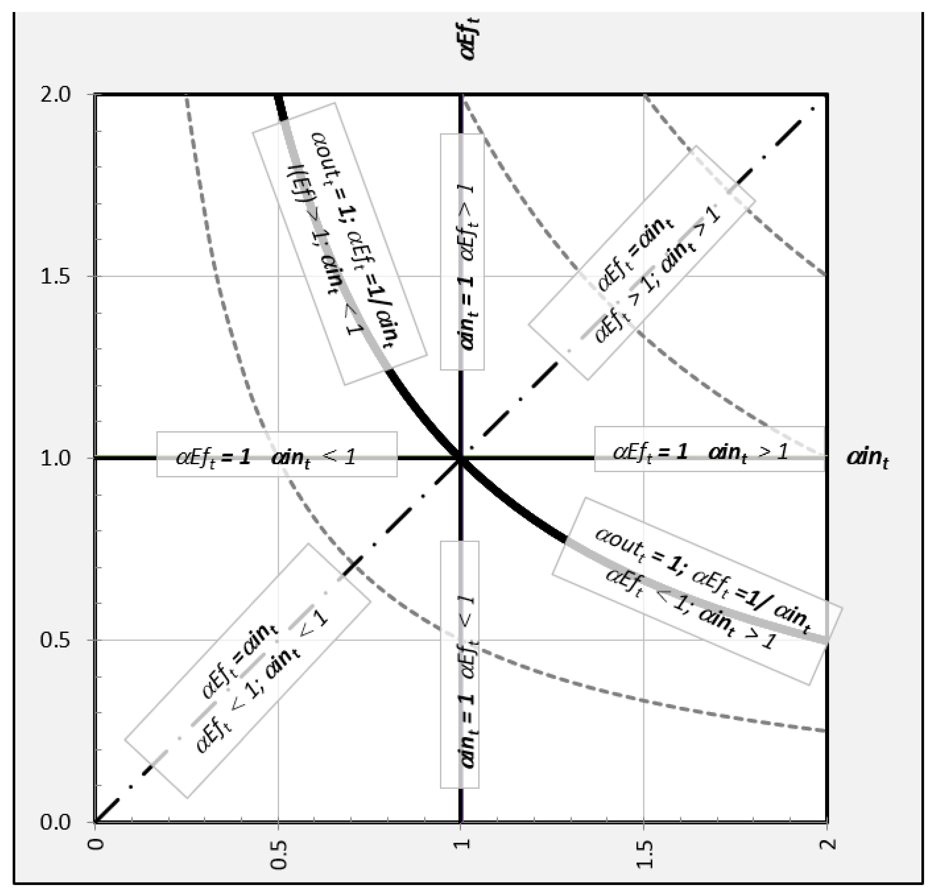
Definition 11. Space for displaying the typology of developments: The relations between the changes in the extensive and intensive factors and the changes in the members of the output sequence αoutt can be effectively expressed using a figure of the coordinates for αint on the x-axis and the coordinates for αEft on the y-axis—see Figure 1. The figure also contains the isoquants of αoutt, i.e., the isoquants representing all of values of αEft and αint, which lead to αoutt having the same specific value (here, 0.5; 1; 2; and 3). These isoquants can be expressed by the relation It is clear from Equation (24) and
Figure 1 that the isoquants of the steady (same) development of output
αoutt are equal–axial hyperbolas. There is constant elasticity on these hyperbolas. Of particular importance is the hyperbola of output stagnation, which passes through the origin of the coordinates (1; 1). All of the isoquants above represent output growth, and all of the isoquants below represent a decrease. For example, the isoquant with value of 2 in
Figure 1 shows all of the combinations of
αint a
αEft, which results in the doubling of the outputs.
Figure 1 illustrates all of the basic types of relations between the development of extensive and intensive factors on the one hand and the development of output on the other. These basic types of relations (basic developments) include:
Definition 12. Pure developments: These are located on the coordinate axes of Figure 1. Growth or decreases in output occur solely due to one of the factors considered, either a purely extensive factor or purely intensive factor. The second factor does not change, i.e.,αint = 1 (for a purely intensive change) orαEft = 1 (for a purely extensive change).
Definition 13. Balanced developments: There are two factors that are considered to act the same, i.e.,αint =αEft. These developments are located in quadrants I and III on a line at a 45-degree angle that intersects the origin of the coordinate axes, i.e., point (1; 1).
Definition 14. Compensation developments: Here both considered factors completely compensate for output stagnation, i.e.,αoutt = 1; therefore,αEft = 1/αint. These developments are found on the hyperbolic isoquant of the stagnation outputs (see above).
Definition 15. Complete stagnation: Complete stagnation (zero development) is characterized byαoutt =αint =αEft = 1, i.e., none of the considered quantities changed during the given period. This situation corresponds to the origin of the coordinates at point (1; 1).
If we characterize each of these developments in greater detail, the following applies:
Definition 16. Pure extensive growth and decline: Pure developments can be differentiated into pure growth and pure decline. For a pure extensive development, whereαEft = 1, pure extensive growth (αint > 1) is found on the positive ray of the x-axis, and pure extensive decline (αint < 1) is represented by the negative ray of the x-axis. For pure intensive development,αint = 1; then, the following applies analogously: pure intensive growth (αEft > 1) is shown by the positive ray of the y-axis, and pure intensive decline (αEft < 1) is shown by the negative ray of the y-axis.
Definition 17. Balanced intensive–extensive growth and decline: For balanced developments (αEft =αint), intensive–extensive growth (αoutt > 1) is represented by the positive part of the line below the 45° angle intersecting the origin of the coordinate axes (i.e., the part in quadrant I), and intensive–extensive decline (αoutt < 1) is represented by the negative part of the line at a 45° angle intersecting the origin of the coordinate axes (i.e., the part in quadrant III).
Definition 18. Intensive–extensive and extensive–intensive compensation. For compensatory development (αoutt = 1, soαEft = 1/αint), it can be distinguished by intensive–extensive compensation—observed in the upper half of the stagnation hyperbola, whereαEft > 1 andαint < 1 apply, or by extensive–intensive compensation—observed in the lower half of the stagnation hyperbola, whereαEft < 1 andαint > 1 apply.
The basic types of developments are crucial for deriving the general typology of the developments, but they are rare in reality. It is not very likely that the output of a system would grow or decline purely intensively or purely extensively or that both factors (
αint and
αEft) would act on the growth or decline of the output exactly at the same rate, nor is it frequent that the output does not change at all (
αoutt = 1) because of the fully compensatory action of both factors. Therefore, it is necessary to focus on mixed types of developments. These are all of the other situations that can arise apart from the basic ones that have just been defined. Graphically, it applies for those with representations in
Figure 1 that lie outside the coordinate axes, outside the line at a 45-degree angle in quadrants I and III intersecting the origin of the coordinate axes, and outside the hyperbolic isoquant for stagnation. These are eight separate spaces that can always be characterized by a triad of inequalities that concurrently determine whether the product grows or not, i.e.,
αoutt > 1 or
αoutt < 1. The first one of the three inequalities determines the relation between
αEft and
αint or (for compensatory development) between one quantity and the inverted value of the other. The second inequality determines whether there is growth or a decrease in the inputs
int, i.e.,
αint > 1 or
αint < 1. The third inequality determines whether there is growth or a decline in the efficiency
Eft, i.e.,
αEft > 1 or
αEft < 1, for example, a space in which
αoutt > 1 and concurrently
αEft > 1/
αint where
αEft > 1 and
αint < 1 is applied represents mixed development, as shown on the area between the positive direction of the
y-axis and the top of the stagnation hyperbola. It expresses the situation of the output growth even though inputs are decreasing. This means that the growth of
Eft not only compensates for the decline
int, but is also sufficient to be the cause of output growth, i.e.,
αoutt > 1.
The relations
αEft and
αint for all of the basic and mixed development types are shown in
Figure 2 and in
Table 1.
The individual spaces shown in
Figure 2 are named so that the names convey reality as accurately as possible. The nomenclature of all of the basic and mixed developments types is based on the following principles:
- -
The nomenclature must cover all development types.
- -
If output grows, the term growth is used; if it falls, the term decline is used; if it does not change, the term pure compensation is used.
- -
All basic developments are referred to as pure.
- -
If both factors (both intensive and extensive) act on growth or if both act on a decline in output, but not equally, the word mainly or predominantly is used, whereas the name of the predominant factor is also used, i.e., mainly intensive growth shows a situation where both factors (αint and αEft) act on growth, but the influence of intensive factors is greater than the influence of extensive factors. Similarly, the term mainly extensive decline describes a situation where both factors (αint and αEft) decline, yet the influence of extensive factors is greater than the influence of intensive factors.
- -
In the designation of opposite developments, where one factor acts on the growth and the other acts on the decline in output, the words compensation or compensatory are used.
- -
If the words intensive and extensive are used in the case of mixed compensatory or pure compensatory developments, the first one used is the one that acts on the growth, and the second one acts on the decline. As an example, the term intensive–extensive compensatory growth thus refers to the situation where intensive factors grow so rapidly that they even compensate for the decline in extensive factors, and they contribute to the output growth, such as in the above-mentioned situation where αoutt > 1 at the same time as αEft > 1/αint while αint < 1 and αEft > 1. Similarly, an intensive–extensive compensatory decline reflects a situation where intensive factors increase while extensive factors decrease at a higher rate, which results in a decline in the output. Pure intensive–extensive compensation using this logic then reflects a state where the intensive factors act on the growth and the extensive factors act on a decline at the same time, such that the result is the stagnation of the output (pure extensive–intensive compensation defines the situation when extensive factors act on growth and intensive factors act on decline such that they once again result in the stagnation of the output).
The names of all of the basic and mixed developments are provided in
Figure 3, which also contains the value of the dynamic intensity indicator and the dynamic extensity indicator (which are derived and explained in
Section 4) related to the development. To make the figure clear, we use the following symbols:
i represents the dynamic intensity indicator, and
e represents the dynamic extensity indicator.
Depending on the location of the point in the appropriate combination of zones, the development of the analyzed system can be clearly characterized.
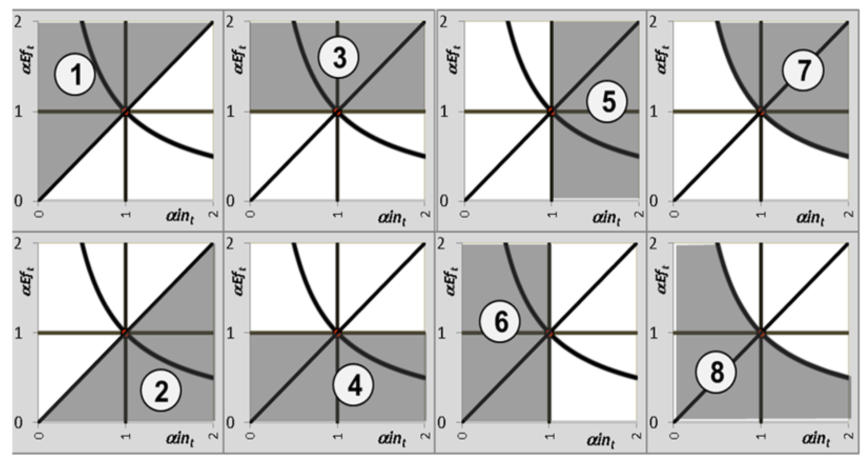
Figure 4 expresses the main different zones qualitatively in the form of eight spaces displaying the quality of the development. The analyzed zone is always displayed in gray and marked with a number. The pictures in the columns (the first one is above the remaining picture, and the second one is below the remaining picture) show zones that complement each other.
Definition 19. Characteristics and definition of the zones of a system development.
Zone 1: intt ≥ expt; intensive factors exceed extensive ones or are equal at the diagonal boundary of the zones;
Zone 2: intt ≤ expt; extensive factors exceed intensive ones or are equal at the diagonal boundary of the zones;
Zone 3: intt ≥ 0; intensive factors contribute to the output growth or are zero at the horizontal boundary of the zones;
Zone 4: intt ≤ 0; intensive factors contribute to the output decline or are zero at the horizontal boundary of the zones;
Zone 5: expt ≥ 0; extensive factors contribute to the output growth or are zero at the vertical boundary of the zones;
Zone 6: expt ≤ 0; extensive factors contribute to the output decline or are zero at the vertical boundary of the zones;
Zone 7: αoutt ≥ 1 or βoutt ≥ 0; output grows or stagnates at the hyperbolic boundary of the zones;
Zone 8: αoutt ≤ 1 or βoutt ≤ 0; output decreases or stagnates at the hyperbolic boundary of the zones.
Each specific point is always located in four zones. For example, if there is a point in the overlap of zones 1, 3, 6, and 7, this means that the output growth is the result of efficiency. The growth of the intensive factors (efficiency) not only compensates for the decline in extensive factors (inputs), but results in output growth.
4. Derivation of Dynamic Indicators of Extensity and Intensity Based on the Identity of the Coefficients
As mentioned in the previous section, dynamic intensity and extensity indicators express how the changes in intensive factors (the change in efficiency,
Ef) or extensive factors (the change in inputs,
int) contribute to a change in output (
out). The key relation for deriving the indicator is Equation (13), which can be logarithmically converted to the following additive relation (25):
The dynamic intensity indicator expressing the share of the influence of the intensive factor on the system development can be written for situations when both the output as well as the efficiency and inputs grow as:
The extensity indicator can be expressed analogously
or as
Since only output growth
(outt),
(int) i
(Eft) is currently being considered, it is possible to derive the value of the intensity indicator for pure intensive and extensive growth. For pure intensive growth
, the output coefficients
(outt) and the efficiency
(Eft) are equal to
and the value of the intensity indicators
(intt) in Equation (26) should acquire a magnitude of 1 or 100% for pure intensive growth. This is clear from the fact that in Equation (26), the numerator and denominator will be identical, and therefore,
intt = 1. At the same time, it applies
αint = 1, which can only be fulfilled using Equation (28) when extensity
extt = 0 or 0%, i.e., the numerator of Equation (28) is equal to 0, whereas the denominator is not equal to zero.
For pure extensive growth, the following applies:
the value of the extensity indicator
(extt) in Equation (28) for a pure extensive development must have the value of 1 or 100%. The numerator and denominator of Equation (28) are identical in situations with pure extensive development. At the same time,
αEft = 1, which can only be fulfilled as part of Equation (26) in cases where
intt = 0 or when the intensity is 0%. This is because Equation (26) has a null numerator and a non-zero denominator.
For symmetric pure intensive–extensive growth,
the value of the intensity indicator
(intt) in Equation (26) is 0.5 or 50% for this development, meaning that the extensity indicator
(extt) in Equation (28) will have a magnitude of 0.5 or 50%.
If we also analyze declines using the same logic, we can once again start from Equations (26) and (28). Only one factor is involved in the fall of both pure declines and causes the output (outt) to decrease. In a way, pure intensive decline is the opposite of pure intensive growth, which has been assigned values of intt = 1, i.e., 100%, and extt = 0, i.e., 0%. The opposite development should be expressed with the opposite indicator value, and once again, only the intensive factor contributes 100% to its development, albeit by its decline. Thus, Equations (26) and (28) must be adjusted so as not to change the very logical results for growth, but so that the equations generate intt = −1, i.e., −100%, and extt = 0 for the pure intensive decrease. In Equations (26) and (28), we can use the αoutt from Equation (25) once again, whereas we assigned both logarithms in the denominator to have an absolute value. This does not change anything with the previous results, but for the pure intensive decrease, the equations that have been adjusted in this way will generate the required values for the intensity indicator, i.e., intt = −1.
Definition 20. Dynamic intensity indicator.
Definition 21. Dynamic extensity indicator.
We will now verify whether Equations (33) and (34) will generate values of the dynamic intensity and extensity indicators in the remaining developments according to the general typology of developments. For a pure extensive decrease, which is subject to the equation
Equations (33) and (34) generate dynamic indicator values of
intt = 0 and
extt = −1, i.e., −100 %. An intensive–extensive decrease caused by the same decrease in both factors is subject to the equation
and Equations (27) and (29) transition into the relations in Equations (37) and (38), which differ from Equations (27) and (29) by the sign of the exponent. Equations (37) and (38) apply to all of the points in quadrant III:
It remains to be seen which values both indicators take in cases of complete compensation (on the compensatory hyperbola,
αoutt = 1
= αint ⋅ αEft), in which the following equation in applied:
In pure intensive–extensive compensation, there is a positive expression, ln αEft, and a negative expression, ln αint. With pure extensive–intensive compensation, it is the opposite. If the sum of the logarithms of αEft and αint equal 0, then they must be equal in terms of their absolute value. Therefore, in Equations (33) and (34), the denominator is always twice the value in the numerator. The values of the dynamic indicators (intt) and (extt) always take values of 0.5 with pure compensations, and the sign is determined by the numerator. For pure intensive– extensive compensation, intt = 0.5, i.e., 50%, and extt = −0.5, i.e., −50%. For pure extensive–intensive compensation, intt = −0.5, i.e., −50%, and extt = 0.5, i.e., 50%.
Figure 5 shows the values of the intensity and extensity indicators for all of the basic and mixed developments in relation to each other. The indicator (
extt) is drawn on the
x-axis, and the indicator (
intt) is drawn on the
y-axis. The figure is based on the relation between the indicators resulting from Equations (33) and (34), which takes the following form:
The derivation of the indicators comes from the nonlinear model of reality. It is clear from
Figure 5 that the magnitude of the dynamic indicators of intensity
intt and extensity
extt is normed at an interval of (−1; 1). For all of the basic developments, it is possible for the values of both dynamic indicators to be any of the following numbers: −1, −0.5, 0, 0.5, or 1, and in all cases, the values correspond to the derived typology of developments. The values of the indicators are symmetrically distributed around the axis of quadrants I and III. The indicators can be used wherever there are the changes (different values) in the output and input variables and where there are the changes in efficiency that are measurable by changes in the shares of the outputs and inputs. The only fundamental prerequisite is that the values of the members of the time sequence of the inputs must be positive rational numbers, i.e., 0 <
int, and that the values of the members of the time sequence of the outputs must also be non-negative, i.e., 0 ≤
outt.
These indicators can be used as a suitable base for decision-making models. Contemporary models (see, e.g., [
25] for details) do not pay sufficient attention to issues of intensity and extensity during system development. The intensity of a system can be seen as proof of appropirate system development, and it should be added to inventories of other signs of successful development, such as system reliability. It is not sufficient to rely only on efficiency as defined by Equation (3). The value of efficiency can, for instance, still be the same, but the number of inputs and outputs decrease proportionally. In that case, the system shrinks and may be too small to be able to compete with other systems. These indicators generally describe what happens in a system. If the correct number of inputs and outputs is used, then the indicators are able to reveal the positive/negative development of the system as well as major events within the system, including periods of system development to be investigated by the theory of catastrophes (see, [
26,
27,
28] for details). Long periods of time in which the dynamic intensity indicator has a value of zero or a negative value indicates that the system was hit or has experienced problems, including serious catastrophes such as sudden sharp changes in the price of the inputs or outputs, [
29], traffic accidents [
30], etc.
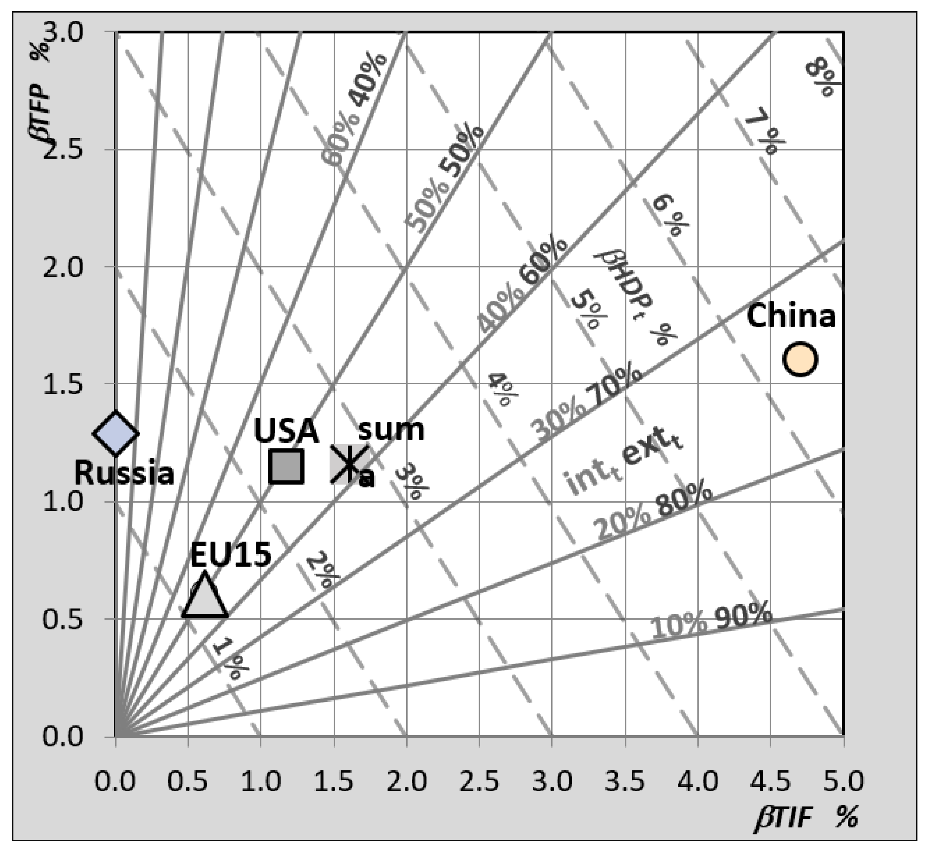
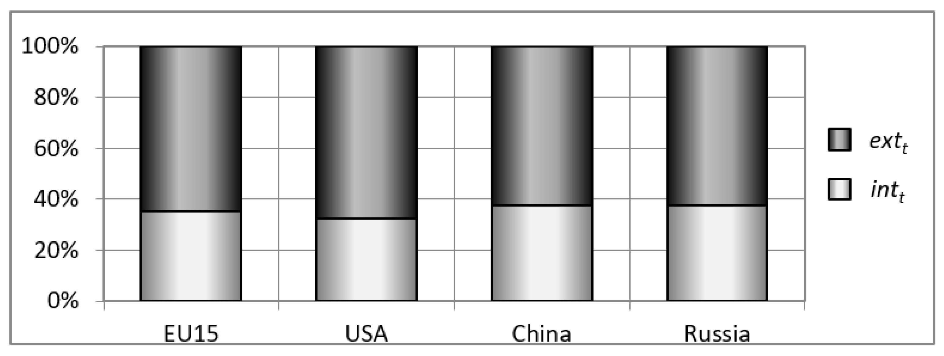
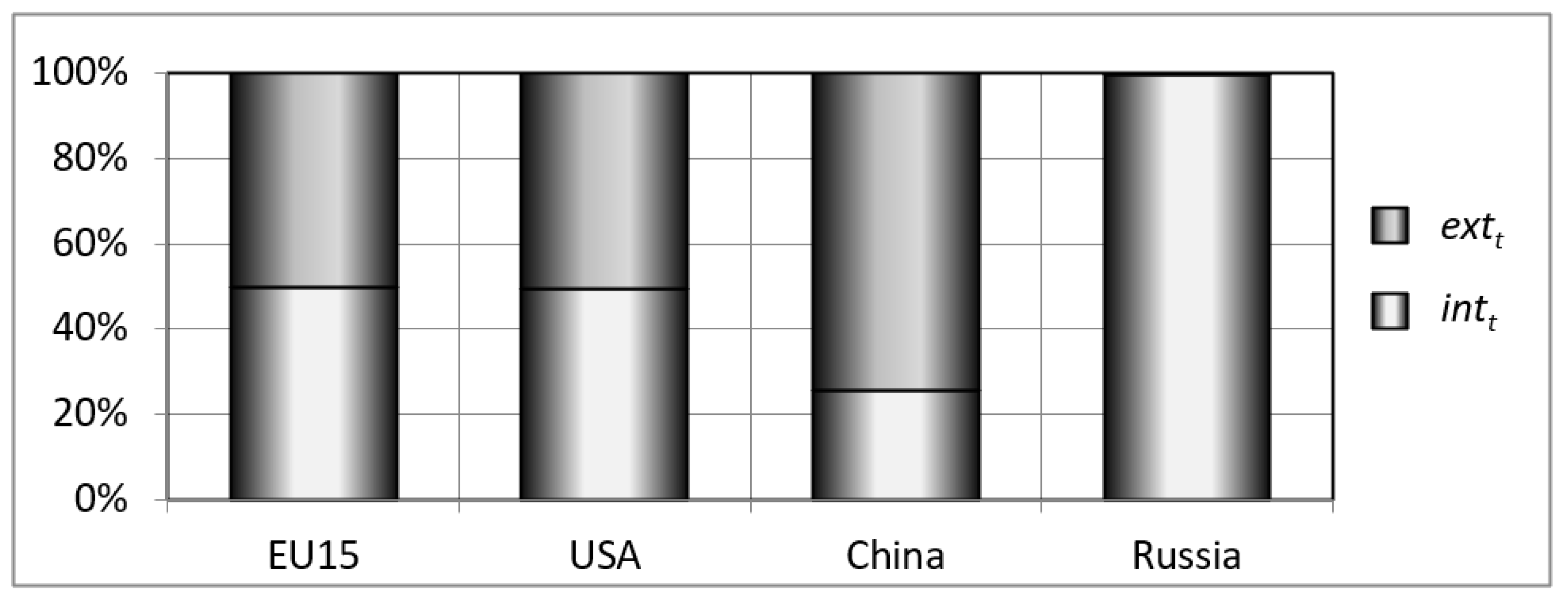
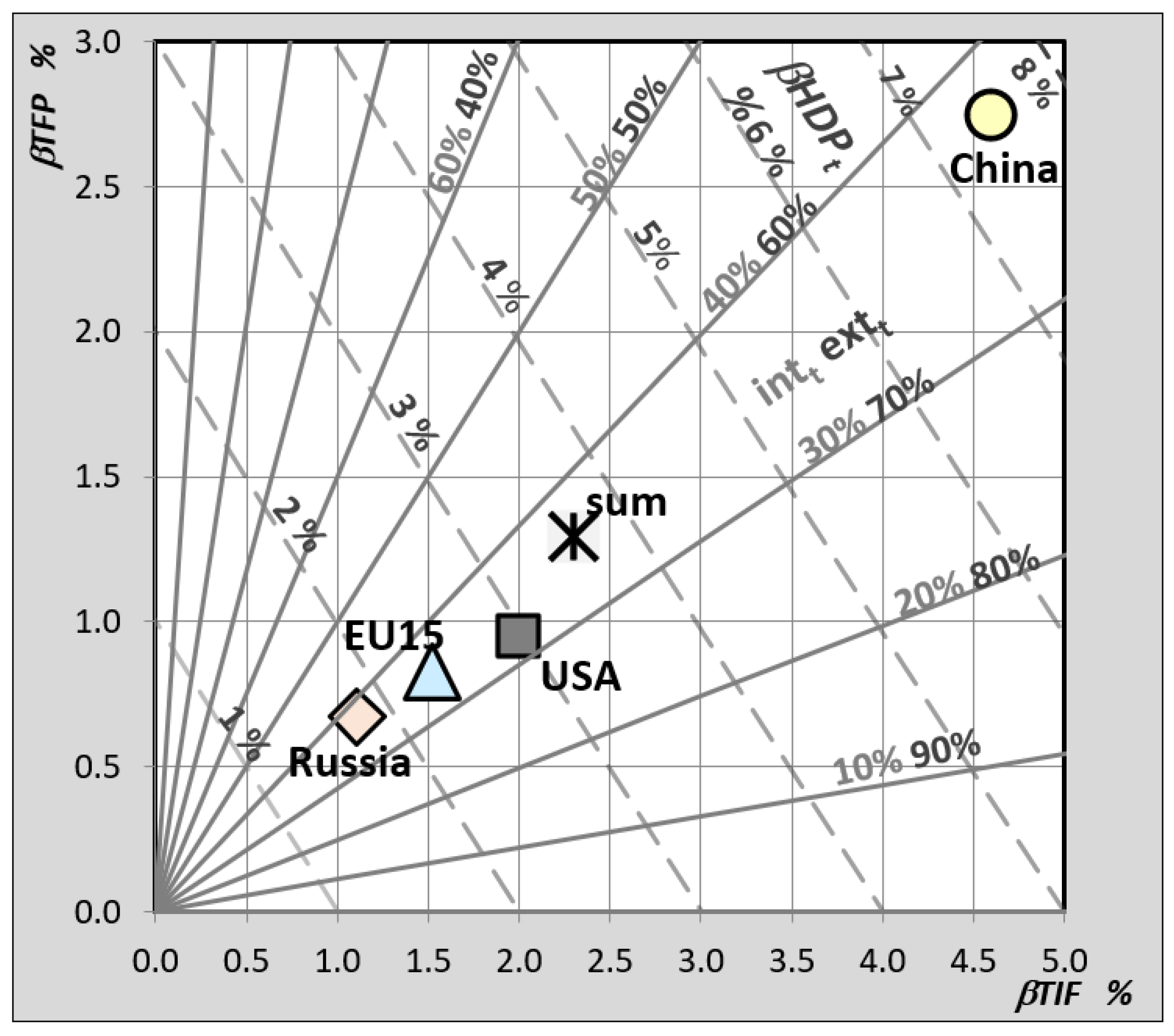
6. Discussion
How accurate are the dynamic intensity and extensity indicators? Our article shows that indicators can easily and understandably describe how a system develops and if the change in its output mainly depends on the change in the number of inputs (the quantitative or extensive change) or the quality of inputs (the qualitative or intensive changes). To be able to clearly state that a system is mainly developing extensively or intensively, it is necessary to analyze not only the quantities (amount) of outputs and inputs, but also their quality. It is possible that neither the outputs nor inputs for a specific period are comparable to the outputs and inputs for another period. This can lead to situations where the indicators do not provide accurate results. In cases where the inputs grow faster than outputs, the dynamic intensity indicator is negative. However, when the quality of the outputs improves significantly, and even when there is a smaller amount of output, greater satisfaction can be achieved for system members or other subjects. Overall, this kind of development can be considered as intensive, but the intensity indicator shows the opposite. The solution in these situations lies in the appropriate choice of output. These should not be just physical units, but units embodying a quality. However, especially in cases of economic systems with inputs and outputs that are usually expressed in monetary units, their value can be biased by inflation or other factors. To obtain accurate values of the dynamic intensity and extensity indicators, stable input and output prices should be used, or other adjustments reflecting the processes in the given economic system and leading to the correct values of input and output should be realized. Other suitable data can include research and development expenditure, patent applications, high-technology exports, the number of researchers in R&D, etc. We did not use these data in our investigation in
Section 5 due to the difficulty of obtaining them. However, it is necessary to emphasize that the indicators that come from data can only correctly describe whether a system has developed intensively or extensively if the data accurately and truthfully describe reality.
Questionable results can be also achieved if the changes in the inputs and outputs of a system are quite small. Just imagine a situation where the output changes from 2 to 2.2 (by 10%) and where the input grows from 1 to 1.02 (by 2%). Indicators mainly indicate intensity development, with the dynamic indicator achieving intensity levels of 88.39%. However, such small absolute change cannot confirm that the change is due to effects of intensive factors. If there is almost no system development, then there cannot be reliable intensity or extensity values.
Another problem is if the analysis focuses on changes in the short run period. In the case of the analysis, if the output of a company or the country’s GDP changed intensively or extensively, then misleading values mainly come from the changes between the next periods (e.g., year-on-year). The inputs of economic systems are mostly fixed, and they cannot be changed in a short period of time. The amount of output depends on the demand for system products. If demand falls for a reason beyond the system’s control and the number of inputs does not change, the intensity indicator is negative. However, this may be a short-term fluctuation that does not require special attention. Indicators truthfully describe that something has happened, but they depend on other assessment to determine whether the system should respond to the event and how.
The above-mentioned situations show that values of the indicators collected over a long period of time (in the case of economic systems, 3 or more years) are much more accurate. Generally, it must be emphasized that the value of dynamic intensive indicators should be positive in the long run. A negative value in long run clearly indicates that the system is not developing optimally and will face, sooner or later, serious problems.
Our classification demonstrates that the development of a system’s performance may be positive and its output increases, even when the value of dynamic intensity indicator is negative. This situation is shown in row 6 of
Table 1 (extensive–intensive compensatory growth)—the decline in intensive factors is offset by an increase in extensive factors. Similarly, the situation shown in row 8 of
Table 1 (pure intensive–extensive compensation) is also dangerous, as intensive factors are declining, but extensive factors are increasing at the same rate, thereby offsetting the decline in intensive factors. In this case, the system’s output does not change. The management of the system can remain complacent in both situations, resulting in the belief that everything is in order. Neither extensive–intensive compensatory growth nor pure intensive–extensive compensation is sustainable in the long run. As we already mentioned, the amount of the inputs will become depleted at some point, and the system will not have other resources for its development. Other situations described in
Table 1 may also be alarming, such as the situation in row 4, especially if the value of the dynamic extensity parameter is a much higher rate than the value of the dynamic intensity parameter in the long term. This situation indicates possible stagnation and the probability of the failure in the competition with other systems.
Row 11 of
Table 1 shows a situation where the growth of extensive factors cannot offset the decline in intensive factors; rows 12 and 14 show a decline in both intensive and extensive factors; while row 15 describes a decline in extensive factors and no change in intensive factors. All of these situations mean a decrease in the system’s output. In that case, a system should consider steps to increase the value of the dynamic intensity parameter. If the system is a firm, it must be emphasized that standard business evaluation methods such as financial analysis (e.g., [
32]) need not reveal that the firm has not developed intensively (for details see [
33]). Therefore, the indicators should be used as an additional source for the firm’s analysis.
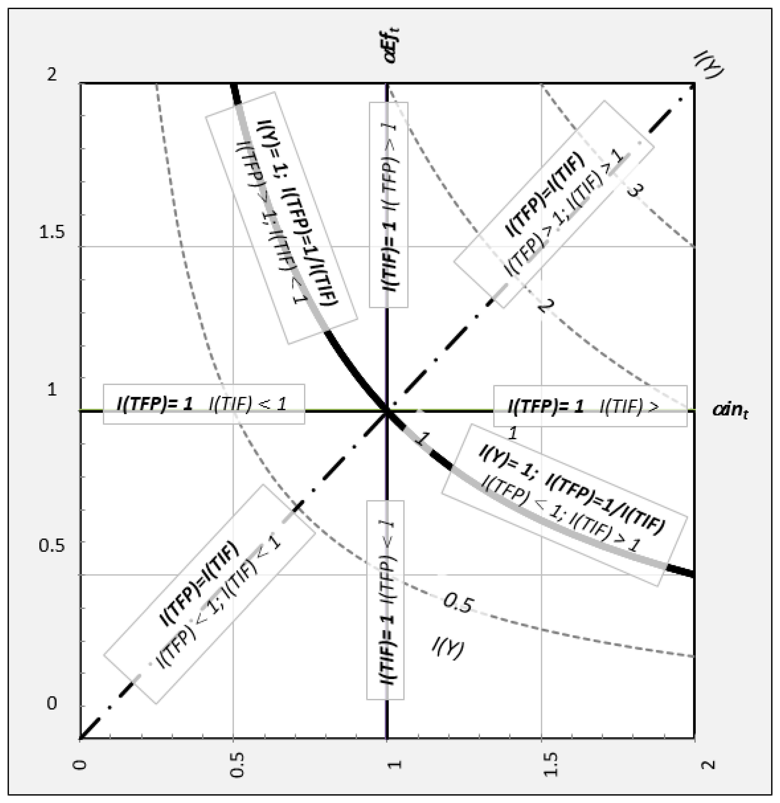
Indicators can be also used for other issues. If a firm wants to know how changes in output and price contribute to the change in total revenues (TR), one parameter (e.g., dynamic intensity indicator) can express the impact of the price changes, and the second one can express the impact of quantity changes. The results are, again, compared to the elasticity that is used for this task, easily understandable, and cover all possible situations, such as if price decreased but quantity increased, resulting in the TR increasing, or if price increased but quantity also increased thus, increasing TR. Another example of using the parameters is investigating how changes in speed (speed can be seen as an intensity parameter) contributes to changes in distance.


