Abstract
A system of mathematical equations was developed for the calculation of the natural frequencies of helical springs, its predictions being compared with finite element simulation with ANSYS®. Authors derive the general equations governing the helical spring vibration relative to the Frenet trihedral representing the normal, binormal and tangent unit vectors to the spring medium line. The dispersion relation has been obtained to model a wave traveling along the axis of the wire.
MSC:
70B15
1. Introduction
Helical springs are one of the most frequently used elastic elements in mechanical engineering. They are used in the most diverse structures as elastic energy accumulators supplementing damping devices, e.g., automobile or railroad suspensions, and in advance and return devices, e.g., camshafts and valves of internal combustion engines (Wahl [1], Shigley [2]; Kobelev [3]). One of the spring failure modes is caused by resonance vibration that occurs when the spring is excited with a periodic signal of frequency equal to its natural frequency.
Love [4] develops equations to study the static response of helical springs subjected to large deformations. Stokes [5] investigates vibrations in the case of a spring subjected to shock loads. Gironnet and Louradour [6] determine more precise expressions for the calculation of the natural frequencies of the helical spring. There are several numerical methods to determine the natural frequencies, the main ones being: the transfer matrix method (Yildirim [7]), the dynamic stiffness formulation (Lee [8]), and the pseudo-spectral method (Lee [9]). Becker [10] determines with the transfer matrix method the resonant frequencies of a spring subjected to an axial compression load. Jiang [11] studies forced vibrations and wave propagation in springs using the Laplace transform.
Wahl [1] already proposed in the middle of the 20th century the equations that are widely used today for the design of springs. Among these equations, Equation (1), which provides the stiffness constant of the spring subjected to an axial force, and Equation (2), which provides the natural frequency of the spring placed between two parallel flat plates, stand out.
where kWahl is the spring axial stiffness, G is the shear modulus of elasticity, d is the wire diameter, D is the helix diameter and N is the number of active coils.
Where f is the natural harmonic frequencies of a spring in Hz, and W is the mass of the spring in kg. The fundamental frequency is determined for and is usually the most important frequency in practice. Replacing in Equation (2) the value of the axial stiffness we obtain Equation (3) also called Harignx’s equation [12], who experimentally verified its validity.
R being the helix radius and ρ the density of the material.
Equation (3) indicates that for a given material, the fundamental frequency of a helical spring is proportional to the wire diameter and inversely proportional to the product of the helix diameter and the number of active coils, i.e., the resonance frequency of the spring depends on all the spring design parameters. If a higher frequency is desired for the same spring diameter, it is sufficient to increase the wire diameter (this increases the spring stiffness), and vice versa. If you want to vary the resonance frequency while keeping the wire diameter constant, just change the spring diameter or the number of coils of the spring. All the expressions shown above are raised with respect to an inertial reference system whose main X axis coincides with the symmetry axis of the helical spring.
By design of the machine itself, the spring is always inserted between two masses in relative oscillatory motion and its function is to keep them away from each other ensuring at all times that they do not come into contact. The design of the helical spring depends directly on the inertia between the masses at any given moment. In addition to the diameter of the wire and the spring itself, the number of coils and the pitch are responsible for achieving non-interaction between the mechanical elements in relative motion.
It is interesting to note that the behavior of the spring changes radically when its operation is associated with a mass much greater than that of the spring itself. For example, in the damping systems of a railway bogie such as the one in Figure 1. In that case, the mass of the spring is much lower than the mass of the railway car it is supporting and Equations (2) and (3) are no longer valid. Den Hartog [13] shows that in that configuration the natural frequency follows Equation (4).
where g is the gravitational constant and δest is the static deflection of the spring under the weight of the suspended load.
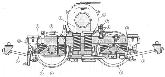
Figure 1.
Damping springs of a railway bogie (Díaz [14]).
Sauvage [15] and Campedelli [16] studied in detail the behavior of the springs of a bogie and simulated in finite elements the anomaly presented by the springs during axial compression called “effort de chasse”. This anomaly consists of a rotation and a lateral displacement appearing on the bearing surface of the spring. The “effort de chasse”, also called transverse flexibility of the spring, is caused by the forces and moments that appear at the ends of the spring during its axial compression. Campedelli [16] determines that the transverse flexibility is determined by both the geometry of the spring end and the way in which the gap between the coils closes during axial compression. The “effort de chasse” is an interesting anomaly in railway suspension springs since in their displacement the springs could interfere with other mechanical elements of the bogie generating interferences and breakages. To avoid this, the railway standard [17] requires a test for the springs of the highest category according to the scheme in Figure 2a. From the test, both the direction and the transverse bowing force (Φc) of the spring subjected to a defined axial load are obtained. The direction of the transverse direction is marked on the spring by a permanent system to take it into account in its mounting on the bogie. Figure 2b shows an example of a bogie spring assembly compensating for the spring bowing forces.
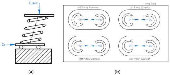
Figure 2.
“Effort de chasse” or transverse flexibility: (a) schematic of the test device; (b) mounting on a spring bogie compensating the “effort de chasse”.
Kobelev [18] also studies another type of anomaly in the behavior of springs such as the transverse vibration of the spring once it enters into oscillations close to resonant frequencies. Kobelev [18] found that the fundamental natural frequency of transverse oscillations turns to be to zero when the lateral buckling of the spring occurs.
Yildirim [19] demonstrates that Equation (1), which is usually used to determine the spring stiffness, is only valid for spring angles α ≤ 10°. Figure 3a shows the spring geometry indicating the position of the angle α.
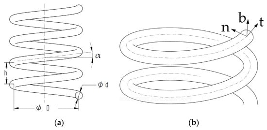
Figure 3.
Helical spring: (a) geometrical parameters; (b) Frenet trihedral.
Yildirim [19] indicates that Equations (1) and (2) only take into account the effect of the torsion of the spring section when compressing it. However, as Yildirim [19] points out when the axial compression force acts, both stresses due to torsion and bending moment and forces normal and shear to the section appear. These last three effects are negligible for spring angles α ≤ 10° where the torsional effect dominates. Yildirim [19] proposes a global equation to determine the deformation of the spring subjected to an axial force. Additionally, Kato [20] proposes recently an equation outside the elastic range to determine large spring deformations.
In general, the previous authors focus the study of the spring behavior using a conventional Cartesian system in which the static or dynamic displacements are referred to as the first axis of symmetry of the helical spring, X. With this methodology the global behavior of a spring as a whole can be known with precision, i.e., constituted by a series of coils of a certain diameter and a certain thickness of the wire, contemplating in some of the occasions the ending effect.
This type of methodology, therefore, allows us to analyze the elastic effect of the spring as a whole, but it is not able to explain some mechanical behaviors intrinsic to its own constitution, i.e., it does not study the phenomenon occurring in the coil itself. In this way, anomalous spring behaviors such as those described above cannot be fully explained.
In order to achieve a reference system that meets these needs, the Frenet trihedral is used in this article, since it is intrinsic to the wire of the spring itself, configuring a reference system positioned according to the neutral line of the helix of the coil as shown in Figure 3b.
In the present study, the equations of motion of the coil of a helical spring are obtained in order to determine its modes of vibration. This is an original and novel approach since the usual practice is to obtain the modes of vibration of the complete spring referred to as a reference system according to its joint motion. Additionally, a sensitivity analysis has been performed for the main geometrical parameters of the coil: i.e., the helix diameter, the wire diameter and pitch. The obtained vibration modes have been validated satisfactorily with finite element calculations with ANSYS® R17 (release 17).
2. Model of Coupled Bending and Torsional Oscillation in a Spring
2.1. Frenet’s Trihedral
For the approach of the oscillation model of the coil, the coordinate system formed by the Frenet trihedral, intrinsic to the neutral line of the spring, has been considered.
Figure 4 shows a differential element of the length of the curve defined by the midline of the coil of a helical spring. The Frenet trihedral or intrinsic trihedral is positioned on it. It is an orthonormal trihedron () whose components are named tangent, normal and binormal. The tangent vector is oriented to the neutral line of the loop. The normal is directed towards the bending center of curvature of the loop. The binormal vector follows the orientation defined by the other two. The vectors t and n form a tangent plane to the loop, containing the element ds, and perpendicular to the binormal vector which is directed towards the bending curvature of this element.
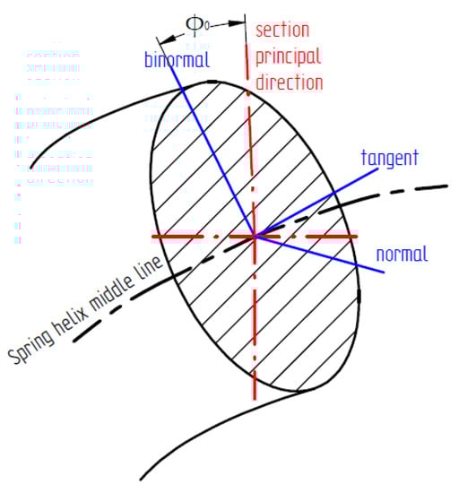
Figure 4.
Intrinsic trihedral and principal directions of inertia of the section.
Considering as a scalar variable the arc length of the midline of the loop(s), we obtain the well-known Frenet–Serret equations, Equation (5), which give us the derivative with respect to s of the components of the trihedral as a function of the curvature of the midline of the coil.
where , and . Where is the bending curvature, the torsional curvature and the angle formed by the principal directions of inertia with the Frenet trihedron.
Equation (5) can be expressed as a function of the vector product of the Darboux vector by the components of the intrinsic trihedron obtaining Equation (6).
where the Darboux vector is defined according to Equation (7):
The variation of any vector function, for example, the rotation and translation of the section, with respect to the length s of the arc follows the expression of Equation (8a) that we will simplify using the notation of Equation (8b) where we will call the tensor associated with the operation .
where is the derivative calculated as if the Frenet trihedron were fixed along the curve. That is, the variation of the function along the curve has two terms, the first represents the variation of the vector within the basis itself and the second represents the variation of the basis itself along the curve.
2.2. Rotation of the Spring Cross-Section
The spring in its natural geometrical configuration undergoes a deformation caused by external forces and moments. The plane cross-section remains plane and we neglect its small deformation. As shown in Figure 5, the cross-section of the deformed part is obtained by a translation of the center and a rotation of the section. Therefore, the point the intersection of the cross-section with the midline, will be transformed into the point (where ) and the perpendicular axes (j,k), coinciding with the normal and binormal of the intrinsic trihedron before the deformation, will become the axes which we also assume to be perpendicular to each other. The axis is obtained as the vector product of the previous ones, .
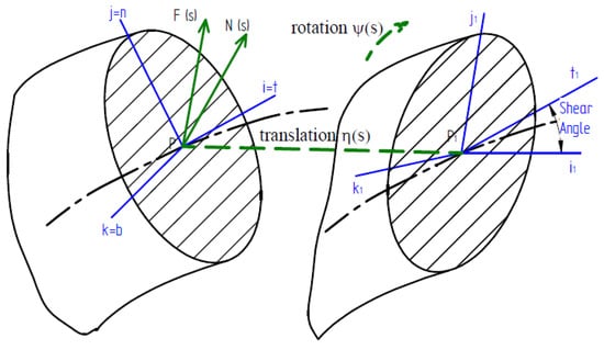
Figure 5.
Schematic of the oscillations of the spring section.
Due to the shear produced by the shear forces, the i-axis is not transformed into the i-axis1 by rotation and translation. Consequently, the tangent vector to a point on the midline of the part will no longer coincide with the first axis of the trihedron as it did in the initial equilibrium state but will form an angle , called the shear angle, proportional to the shear stress. If we do not consider the deformation due to the shear stress, the shear angle is canceled, so that the tangent to the midline of the part will be perpendicular to the section, or what is the same, will coincide with the first axis of the trihedron.
The derivative of with respect to s is given to first order by Equation (9a,b).
where is the tensor associated with the torsional-flector torque increment, E is the modulus of elasticity, G is the shear modulus of elasticity, Ii is the geometric moment of inertia and k1 is the torsion constant. is the vector of internal torque increase. Its first component is the torsional moment, and the other two components are the bending moments in the normal and binormal directions. is the torsional stiffness, is the bending stiffness along the normal axis, and is the bending stiffness along the binormal axis.
2.3. Translation of the Spring Cross-Section
The derivative of the displacement vector with respect to s is given to first order by Equation (10a–c).
where MF is the tensor associated with the forces and ki the shear constants, or the so-called Timoshenko’s k-factors [21]. Being for symmetric sections . is the vector of internal force increment. Its first component is the axial force, and the other two components are the shear forces according to the normal and binormal. is the axial stiffness and is the shear stiffness.
Equations (9a,b) and (10a–c) constitute a system of six scalar equations for the twelve components of . The remaining six equations are obtained from the dynamic study of the system for which the equations of the linear momentum and angular momentum of the part element comprised between s and s + ds are posed.
2.4. Linear Momentum
Considering the linear momentum, the derivative of with respect to s is given by Equation (11).
where is the linear density per unit length.
2.5. Angular Momentum
Considering the angular momentum, the derivative of with respect to s is given by Equation (12a,b), which takes into account the effects of rotational inertia introduced by Rayleigh [22].
Table 1 summarizes the complete system of equations obtained and which describes the behavior of the spring coil subjected to bending and torsion. It consists of four vector equations in linear partial derivatives, non-homogeneous and of second order.

Table 1.
System of Vectorial Equations to model spring behavior.
2.6. Dispersion Relation
If in the Table 1 system of equations we change the variable using Equation (13a–d), we can simulate the movements in time of the spring and then perform a vibration analysis of its oscillatory behavior in the vector variables . We will assume a wave traveling along the axis of the wire. Thus
The new parameters introduced are the wavenumber, k, and the angular velocity of the wave, ω (rad/s). Where the wavenumber k, is related to the length λ of the vibrating wave, with Equation (14).
Substituting the system of equations in Table 1 we arrive at the following system in Equation (15a–d).
where the matrix follows the expression of Equation (16).
Solving for in Equation (15a) and replacing it in Equation (15b), and similarly solving for in Equation (15c) and replacing in Equation (15d) we obtain the following vector Equation (17a,b):
where the matrices are calculated with Equations (18) and (19).
Equation (17a,b) constitutes a system of six equations with six unknowns () and with null independent terms. It is therefore a homogeneous system and for it to have a solution other than the trivial, null solution, it must be verified that its determinant is null, i.e., Equation (20).
Operating the determinant and simplifying we obtain the alphanumerical Equation (21), which would be the dispersion relation, , which relates the length of a wave with its oscillation frequency in the spring coil.
where the coefficients of the polynomial are calculated according to the expressions given in Equation (A1) of Appendix A.
The real roots in of Equation (21) will give us the number of branches of the dispersion equation for each value of the wavenumber k.
If in the dispersion relation obtained for the spring we cancel the independent term, (which is equivalent to making ), we will have the solutions of the wave number shown in Equation (22a,b).
That is to say, there exists a value of the wave number k different from zero (to which corresponds, therefore, a finite wavelength) for which one of the real and positive roots of the dispersion relation (degree 12) cancels, so that the branch corresponding to this solution, for any value of k, is tangent to the x-axis in .
If we do we will obtain the number of branches of the dispersion relation (which will be equivalent to the number of real roots of the equation). For this case, the real and positive branches are determined by Equation (23a–c):
The wave numbers k obtained from Equation (23a–c) are indicators of the spring oscillation modes. Equation (23b) represents the bending oscillations of a differential element of spring length in plane 1, 2 determined by the principal directions of inertia of a cross-section (Figure 6). Equation (23c) represents the torsional oscillations of the differential element around the principal direction 1 of Figure 6. These oscillation modes will be explained also later in the finite elements section.
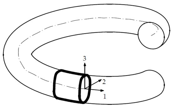
Figure 6.
Spring Oscillation Modes.
The result of the oscillation is bending accompanied by torsion which tends to make the ends of the coil open and close in time, oscillating according to the movement. This is composed of two modes: opening and closing of the ends, the coil remaining at all times inscribed in the original helix of the spring (of diameter D) and the other mode consists of the ends of the coil entering and leaving the original helix of diameter D, forming an ellipse. This last mode responds to the reason why the springs, under certain dynamic conditions, pull the coils out of their original helix, and may impact other elements of the machine, thus affecting its operation. Authors consider this can explain part of the “Effort de Chasse” anomaly described in Section 1.
In this article, we are in the case of a freely oscillating coil. In the case of several coils joined together, it would be necessary to consider the ligatures of their ends as shown in Figure 7 for the end of a squared and ground spring. That is to say, with a helix angle of zero degrees and a flat seat, which allows a better load transfer. The assembly thus defined becomes an oscillatory mode in which the spring as a whole adopts the barrel configuration. Pearson [23] studies the important contribution of the ends to the calculation of the spring natural frequencies.
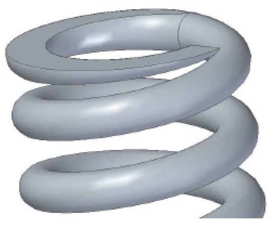
Figure 7.
The end of squared and ground helical spring.
The dispersion relation allows us to obtain the normal modes of oscillation by applying the appropriate boundary conditions. For example, in the case of a helical spring with one end clamped and the other free, the boundary conditions would be as follows: the rotation vector and the translation vector cancel out at the clamped end and the internal torque and the internal stress cancel at the free end. Assuming the clamped end for s = 0 and the free end for s = L, Equation (24) is satisfied which implies that the wave number k takes the values of Equation (25).
Entering the value of k calculated according to Equation (25) in the dispersion Equation (21), the natural oscillation frequencies for the helical spring are obtained.
In order to validate the proposed theoretical model, a comparison with finite elements and with the experimental tests of a helical spring is made below.
3. Application of Finite Elements
The previous calculation performed to obtain the natural frequencies of the system has been compared with the results of the resonance frequencies obtained by numerical simulation. In addition, a complete modal analysis is performed. In order to compare the results, the oscillation modes of the one spring turn are calculated using standard computational methods. The simulations have been carried out by modeling the spring geometry by Finite Elements using ANSYS® software.
A three-dimensional geometry of the helicoid representing the neutral fiber of a helical spring has been faithfully reproduced. The three-dimensional geometry has been generated from SOLID EDGE software, and it has been imported by the FEM software in the *.iges format. The SOLID EDGE software provides flexibility in the modelization and facilitates the actual geometrical definition compared to the CAD tool integrated in ANSYS. The spring is thus reproduced volumetrically.
We proceed to calculate in both cases, i.e., the theoretical model proposed in the previous section with one solved in finite elements, in order to compare the results.
In finite elements, a meshing has been performed using extruded hexahedral elements of 2 mm characteristic size, which represents the circumference of the wire cross-section (10 mm diameter) with 16 nodes in its contour. This results in 6000 nodes per turn, 54,000 nodes for the complete spring and 162,000 degrees of freedom.
The meshing strategy used consists of an extrusion method from the two-dimensional meshing (with quadrilaterals) of the cross-section, which guarantees a regular meshing that avoids geometric distortions of the elements and achieves a low bandwidth for the stiffness matrix, resulting in a better performance of the iterative methods of resolution.
The SOLID185 element has been selected in its homogeneous form, which is frequently used to model three-dimensional structures in ANSYS. The element consists of eight nodes with three degrees of freedom per node: translations in the three directions of space. SOLID185 uses the reduced selective integration method.
The material has been modeled linearly, with steel properties considering Young’s modulus and Poisson’s ratio.
The problem has been plausibly solved using the Lanczos method for the determination of eigenfrequencies and eigenmodes.
In free-free solid conditions, the different natural frequencies of one spring turn belonging to a helical spring, with different helix diameters and wire thickness have been calculated. In all cases, the pitch of the helix has always been the same.
In all cases, the corresponding oscillation modes are studied. Table 2 shows the results. Columns 4 to 9 show the frequency and the mode of vibration. Essentially, the first mode corresponds to an opening between ends, such that the original helix is transformed into an ellipsoidal helix (Figure 8a). In this case, the predominant deformation of the helix is bending. The second mode corresponds to the relative motion between these ends (Figure 8b) but preserves the circumference of the helix, which corresponds to a mode in which the torsional effect of the helix is more predominant than its bending. In this second case, the pitch of the coil would increase significantly.
Table 2.
FEM calculation of the first natural frequencies (Hz) of helical spring.
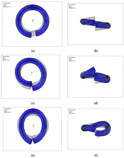
Figure 8.
Modes of vibration of a spring: (a) Bending 1; (b) Torsional 1; (c) Bending 2; (d) Torsional 2; (e) Bending 3; (f) Torsional 3.
From these two basic modes, the deformation profiles are reproduced with increasing inflection points. The third (Figure 8c) and fifth (Figure 8e) modes constitute double bending and triple bending, respectively. Always without leaving the imaginary plane that would contain the spiral if it were a ring in a plane and not helical, but distorting the circumference that defines it. The fourth (Figure 8d) and sixth (Figure 8f) modes constitute double torsion (with one inflection point) and triple torsion (with two inflection points), respectively.
If we continue to search for natural modes at increasing frequencies, increasingly complex deformation profiles with small displacements and numerous inflection points appear.
With respect to the results shown in Table 2, it can be deduced that, in the case of the first resonance mode (bending), keeping the helix diameter constant and varying the wire thickness, the resonance frequency increases with increasing thickness. This is logical because the stiffness of the spring increases. Figure 9 shows this trend. Moreover, as shown in Figure 9, as the diameter of the helix increases, the resonance frequency decreases. Despite maintaining the stiffness, the loop flexes with lower frequency values. A similar situation occurs with the first torsional mode.
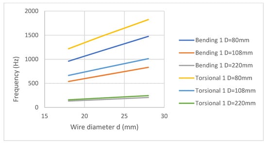
Figure 9.
Sensitivity of the first resonance modes to the wire diameter, d.
Proceeding analogously for the first bending mode, the wire thickness is now kept constant, and the average diameter of the helix is varied (Figure 10). The frequencies decrease as the helix diameter increases. Moreover, as the wire diameter increases, the resonant frequency increases. The situation is repeated for the first torsional mode of vibration. It is a situation analogous to that of the previous paragraph.
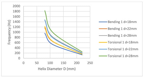
Figure 10.
Sensitivity of the first resonance modes to the helix diameter, D.
Analyzing the variation of the frequency as a function of the variation of the average diameter of the helix, it is observed (Figure 10) that the first bending and torsional mode of the spring decrease as the mass increases due to a higher helix diameter. This has to do with the wire diameter/helix diameter ratio and it can be seen that there is a certain characteristic value of this ratio that linearizes the resonant behavior.
As shown in Figure 9 the relationship between frequencies and wire diameter (d) is linear. This result is consistent with Equation (3).
It has also been considered whether the pitch of the spring can be an influential design parameter when calculating resonances. Figure 11 shows that the pitch variation does not affect the frequencies. Figure 11 shows the different modes obtained and commented.
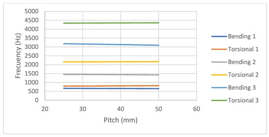
Figure 11.
Sensitivity of the first resonance modes to the pitch of the helix.
Table 3 includes a comparison for the first harmonic of the results obtained with the finite element simulation and the numerical model presented in this paper. The results of the numerical model are obtained by solving in Equation (21) with the wavenumber k calculated with Equation (22b) or Equation (25). In general, it is observed that the numerical model overestimates the frequency values with an average difference of 3%.
Table 3.
Comparison of the numerical model with FEM for the first harmonic (Hz).
4. Conclusions
The study of a single coil has been proposed since, in general, the authors who propose equations to model the vibration behavior of a spring consider the spring as a whole, including its ends, but do not analyze the behavior of the coil itself. From the analysis of a single coil, the singular behavior of the spring known as “effort de chasse” described in the introduction could be justified.
For the study of the vibratory behavior of a spring, an analytical model has been developed based on a reference system consisting of a Frenet trihedron whose tangent vector is the midline of the coil. One of the results obtained from the model is the dispersion relation that relates the wavelength to its oscillation frequency, . Applying the appropriate boundary conditions the dispersion relation allows us to calculate the normal modes of oscillation.
Another of the results obtained is that there is a value of the wavenumber for which the roots of the dispersion equation cancel out. Being and the torsional curvature and the bending curvature, respectively.
Two clear modes of oscillation have been characterized, one in which the coil moves according to the torsion of the cross-section increasing the pitch of the coil, and another bending mode in which it moves by making an opening of its ends so that the original helix is transformed into an ellipsoidal helix.
A spring has been modeled by finite elements with ANSYS® software in order to contrast results with the numerical model, obtaining an average difference of 3% in the fundamental oscillation frequency.
Author Contributions
Individual contributions are as follows: original concept: L.P., A.Q., A.M.G.A. and V.D.; mathematical development: L.P. and A.M.G.A.; implementation, simulation and draft preparation: L.P., A.M.G.A., A.Q. and V.D.; review, editing, validation, and formal analysis: L.P., A.Q., A.M.G.A. and V.D. All authors have read and agreed to the published version of the manuscript.
Funding
This research received no external funding.
Institutional Review Board Statement
Not applicable.
Informed Consent Statement
Not applicable.
Data Availability Statement
Not applicable.
Conflicts of Interest
The authors declare no conflict of interest.
Appendix A
In this appendix, the expressions for the calculation of the coefficients of Equation (21) are indicated. Equation (A1a–g) contains the expressions for the calculation of mi
With Equation (A2a–m) for the calculation of the parameters of the
With Equation (A3a–f) for the calculation of the parameters of the
With Equation (A4a–f) for the calculation of the parameters of the
With Equation (A5a–f) for the calculation of the parameters of the
where Equation (A6a–i) indicates the calculation of the parameters
where Equation (A7a–f) indicates the calculation of the parameters
where Equation (A8a–c) indicates the calculation of the parameters
References
- Wahl, A.M. Mechanical Spring, 2nd ed.; McGraw-Hill: New York, NY, USA, 1963. [Google Scholar]
- Shigley, J.E. Mechanical Engineering Design, 10th ed.; McGraw-Hill: New York, NY, USA, 2015. [Google Scholar]
- Kobelev, V. Durability of Springs; Springer: Berlin/Heidelberg, Germany, 2018. [Google Scholar]
- Love, A.E.H. A Treatise on the Mathematical Theory of Elasticity, 4th ed.; Dover Publications: Mineola, NY, USA, 1927. [Google Scholar]
- Stokes, V.K. On the dynamic radial expansion of helical springs due to longitudinal impact. J. Sound Vib. 1974, 35, 77–99. [Google Scholar] [CrossRef]
- Gironnet, B.; Louradour, G. Comportement Dynamique des Resorts; Techniques de l’Ingénieur: Paris, France, 1983. [Google Scholar]
- Yldirim, V. An efficient numerical method for predicting the natural frequencies of cylindrical helical springs. Int. J. Mech. Sci. 1999, 41, 919–939. [Google Scholar] [CrossRef]
- Lee, J.; Thompson, D.J. Dynamic stiffness formulation, free vibration and wave motion of helical springs. J. Sound Vib. 2001, 239, 297–320. [Google Scholar] [CrossRef]
- Lee, L. Free vibration analysis of cylindrical helical springs by the pseudo spectral method. J. Sound Vib. 2007, 302, 185–196. [Google Scholar] [CrossRef]
- Becker, L.E.; Chassie, G.G.; Cleghorn, W.L. On the natural frequencies of helical compression springs. Int. J. Mech. Sci. 2002, 44, 825–841. [Google Scholar] [CrossRef]
- Jiang, W.; Wang, T.L.; Jones, W.K. The forced vibration of helical spring. Int. J. Mech. Sci. 1992, 34, 549–562. [Google Scholar] [CrossRef]
- Haringx, J.A. On highly compressible helical springs and rubber rods, and their application for vibration-free mountings. Philips Res. Rep. 1949, 4, 49–80. [Google Scholar]
- Den Hartog, J.P. Mechanical Vibrations; Dover Civil and Mechanical Engineering; Courier Corporation: Chelmsford, MA, USA, 1956. [Google Scholar]
- Díaz, V. Automóviles y Ferrocarriles; Universidad Nacional de Educación a Distancia: Madrid, Spain, 2012; p. 287. ISBN 978-84-362-6568-2. [Google Scholar]
- Sauvage, G. Determining the Characteristics of Helican Springs: A simplification for Application in Railway Suspensions. Veh. Syst. Dyn. Int. J. Veh. Mech. Mobil. 1984, 13, 43–59. [Google Scholar]
- Campedelli, J. Modelisation Globale Statique des Systemes Mecaniques Hyperstatiques Pre-Charges Application a un Bogie Moteur. Ph.D. Thesis, INSA Lyon, Lyon, France, 2002. [Google Scholar]
- UNE-EN 13298; Railway Applications. Suspension Components. Helical Suspension Springs, Steel. The European Committee for Standardisation: Brussels, Belgium, 2003.
- Kovelev, V. Effect of static axial compression on the natural frequencies of helical springs. Multidiscip. Model. Mater. Struct. 2014, 10, 379. [Google Scholar] [CrossRef]
- Yildirim, V. Axial Static Load Dependence Free Vibration Analysis of Helical Springs Based on the Theory of Spatially Curved Barx. Lat. Am. J. Solids Struct. 2016, 13, 2852–2875. [Google Scholar] [CrossRef] [Green Version]
- Kato, H.; Suzuki, H. Nonlinear deflection analysis of helical spring in elastic-perfect plastic material: Application to the plastic extension of piano wire spring. Mech. Mater. 2021, 160, 103971. [Google Scholar] [CrossRef]
- Timoshenko, S.P. On the correction for shear of the differential equation for transverse vibrations of prismatic bars. Philos. Mag. 1921, 41, 744–746. [Google Scholar] [CrossRef] [Green Version]
- Rayleigh, J.W.S. The Theory of Sound; Dover Publications: Mineola, NY, USA, 1945. [Google Scholar]
- Pearson, D. Modelling the ends of compression helical springs for vibration calculations. Proc. Inst. Mech. Eng. 1986, 200, 3–11. [Google Scholar] [CrossRef]
Publisher’s Note: MDPI stays neutral with regard to jurisdictional claims in published maps and institutional affiliations. |
© 2022 by the authors. Licensee MDPI, Basel, Switzerland. This article is an open access article distributed under the terms and conditions of the Creative Commons Attribution (CC BY) license (https://creativecommons.org/licenses/by/4.0/).