Representation Theorem and Functional CLT for RKHS-Based Function-on-Function Regressions

Abstract

We investigate a nonparametric, varying coefficient regression approach for modeling and estimating the regression effects caused by two functionally correlated datasets. Due to modern biomedical technology to measure multiple patient features during a time interval or intermittently at several discrete time points to review underlying biological mechanisms, statistical models that do not properly incorporate interventions and their dynamic responses may lead to biased estimates of the intervention effects. We propose a shared parameter change point function-on-function regression model to evaluate the pre- and post-intervention time trends and develop a likelihood-based method for estimating the intervention effects and other parameters. We also propose new methods for estimating and hypothesis testing regression parameters for functional data via reproducing kernel Hilbert space. The estimators of regression parameters are closed-form without computation of the inverse of a large matrix, and hence are less computationally demanding and more applicable. By establishing a representation theorem and a functional central limit theorem, the asymptotic properties of the proposed estimators are obtained, and the corresponding hypothesis tests are proposed. Application and the statistical properties of our method are demonstrated through an immunotherapy clinical trial of advanced myeloma and simulation studies.

1. Introduction

Modern biomedical technology has made it possible to measure multiple patient features during a time interval or intermittently at several discrete time points to review underlying biological mechanisms. Functional data also arise in genetic studies—a massive amount of gene expression data is recorded for each subject and could be treated as a functional curve [1]. Functional data analysis provides distinct features related to the dynamics of cellular responses and activity and other biological processes. Existing methods, such as projection, dimension-reduction, and functional linear regression analysis, are not adapted for such data. Overviews can be found in the book by Horváth and Kokoszka [2] and some recently published papers such as Yuan et al. [3] and Lai et al. [4].

Ramsay and Silverman [5], Clarkson et al. [6], and Ferraty and Vieu [7] introduced some basic tools and widely accepted methods for functional data analysis; Horváth and Kokoszka [2] established some fundamental methods for estimation and hypothesis testing on mean functions and covariance operators of functional data. The topics are broad and the results are in depth. Conventionally, each data curve is assumed to be observed over a dense set of points, often over thousands of points, then smoothing techniques are used to produce continuous curves, and these curves are treated as completely observed functional data for statistical inference. In contrast with those assumptions, we consider the more practical issues in which the data curves are only observed at some (not dense) time points, and the observed data curves are actually interpolations at those observed points. Of course, a relatively large sample size is needed for sparse observations. The effects of both number of observation points and sample size are also considered in our analysis.

For analyzing longitudinal data, Zeger and Diggle [8] considered a semiparametric regression model of the form, with longitudinal observations

$$Y\left(t\right)=X^{\prime }\left(t\right)\beta +\theta \left(t\right)+ϵ\left(t\right),t\in \mathcal{T},$$

(1)

where $Y\left(t\right)$ is the response variable, $X\left(t\right)$ is the $p\times 1$ covariate vector at time t, $\beta$ is a $p\times 1$ constant vector of unknown regression coefficients, $\theta \left(t\right)$ is an unspecified baseline function, $ϵ\left(t\right)$ is a zero-mean stochastic process, and $\mathcal{T}$ represents the observation interval. Under this model, Lin and Ying [9] estimated $\beta$ via a weighted least squares estimator based on the theory of counting processes; Fan and Li [10] further studied this model using a weighted difference-based estimator and a weighted local linear estimator followed by statistical inference, as discussed in Xue and Zhu [11].

For functional data analysis, the data are often represented by $(y_i,x_i(·))$$(i=1,\dots ,n)$, and the model is [12,13,14]

$$y_i={\int }_{\mathcal{T}}\beta \left(t\right)x_i\left(t\right)dt+{ϵ}_i.$$

(2)

Some researchers considered the following model [2,5,15]

$$y_i\left(t\right)={\int }_{\mathcal{T}}\beta (s,t)x_i\left(s\right)ds+{ϵ}_i\left(t\right).$$

(3)

To estimate $\beta (·,·)$, assume there are basis $\left\{{\xi }_k\right\}$ and $\left\{{\eta }_k\right\}$, which span the spaces of the $\left\{x_i(·)\right\}$ and $\left\{y_i(·)\right\}$, respectively. The estimate of $\beta (·,·)$ of the form is given by

$$\widehat{\beta }(s,t)=\sum _{i=1}^k\sum _{j=1}^r{b}_{ij}{\xi }_i\left(s\right){\eta }_j\left(t\right),$$

and $b_{ij}$ is estimated by minimizing the residual sum of squares ${\sum }_{i=1}^n\left|\right|y_i-\int \widehat{\beta }(s,t)x_i\left(s\right)ds{\left|\right|}^2$. Although the resulting estimator is useful, a representation theorem for such an estimator is hard to obtain, and hence the asymptotic distribution of this approach is not clear. Yao, et al. [15] investigated a functional principle component method for estimation of model (3) and obtained consistent results. Müller and Yao [16] studied a variation of the above model in the conditional expectation format.

The smoothing spline method is popular for curve estimation. The function curves can be estimated at any point, followed by the computation of coefficients. However, the asymptotic property of estimators based on the spline method is tough to handle. For natural polynomial splines, the number of knots is the number of untied observations, which is sometimes redundant and undesirable. B-splines only require a few (the degree of the polynomial plus two) basis functions and are easy to implement [17,18,19]. Another method is local linear fit [20,21,22], but the difficulty is in choosing the bandwidth, especially when the observation points are uneven. Therefore, in this paper we employ reproducing kernel Hilbert space (RKHS), a special form of spline method in which the turning point from curve estimation to point estimation Yuan and Cai [12] explored its application on functional linear regression problem, and Lei and Zhang [23] extented it to RKHS-based partially functional linear models. In general, one needs to choose a set of (orthogonal) basis functions and the number of basis for functional estimations, while with RKHS one only needs to determine the kernel(s) of RKHS. Furthermore, the Riesz presentation theorem shows that any bounded linear function can be reproduced as a representer based on the RKHS kernel with a closed form.

However, existing RKHS methods often meet obstacles when choosing different norms and the corresponding optimization procedures. Although using a carefully selected norm in the optimization criterion has the advantage of interpretation, it suffers in that the resulting regression estimator generally needs the computation of an inversion of a large matrix (the same as the sample size). Moreover, most of the existing methods, including the aforementioned RKHS methods, are designed for the case where the observed data are sampled from a dense rate and are limited to models in which either the response or predictors are functions. New methods for estimation and hypothesis testing of regression parameters for the more general case where both the response and predictors are functions with sparsely observed data are needed. To address these problems, we propose a new RKHS method with a unified norm to characterize the RKHS and the optimization criterion for function-on-function regression. Although the statistical interpretation of this optimization criterion is not fully clear, with a simple closed form of the estimated regressors under a general function-on-function regression model, this optimization is more computationally reliable and applicable without the need of computing the inverse of a massive matrix. By establishing a representation theorem and a functional central limit theorem based on the proposed model, we obtain the asymptotic distribution of the estimators. Hypothesis testing of the underlying curves is proposed accordingly.

The remainder of this paper is organized as follows. Section 2 describes the proposed method for the estimation and hypothesis testing of regression parameters for functional data via the reproducing kernel Hilbert space and establishes some theoretical properties. Simulation studies and a real-data example to demonstrate the effectiveness of our proposed method are given in Section 3 and Section 4, respectively. Section 5 gives some concluding remarks, and all technical proofs are left in the Appendix A.

2. The Proposed Method

We consider the observed data $\left\{(y_i\left(t_{ij}\right),{\mathbf{x}}_i\left(t_{ij}\right)),j=1,\dots ,m_i;i=1,\dots ,n\right\}$. The underlying data curves $(y_i(·),{\mathbf{x}}_i(·))$ are iid copies from $\left(y\right(·),\mathbf{x}(·\left)\right)$, where $y(·)$ and $\mathbf{x}(·)={(x_1(·),\dots ,x_d(·))}^{\prime }$ are random curves on some region T. The observation times $t_{ij}\in (0,T]$ are generally assumed to be different for each subject i for some $0<T<\infty$. We assume that time points $m_i$ ($i=1,\dots ,n$) are iid copies from some integer-valued random variable m, and given $m_i$, the time points $t_{ij}$ for ($j=1,\dots ,m_i$) are iid copies from a positive random variable G, with its support on $(0,T]$. For each individual, the observed data $(y_i,{\mathbf{x}}_i)$ can be interpolated as curves $({\widehat{y}}_i,{\widehat{\mathbf{x}}}_i)$ on T. We assume the following model for the observed data

$$y_i\left(t\right)={\mathbf{\beta }}^{\prime }\left(t\right){\mathbf{x}}_i\left(t\right)+{ϵ}_i\left(t\right),E\left[{ϵ}_i\left(t\right)\right]=0,(i=1,\dots ,n),$$

(4)

where $\mathbf{\beta }(·)={({\beta }_1(·),\dots ,{\beta }_d(·))}^{\prime }$ are the true regression coefficient functions for the covariates ${\mathit{x}}_i(·)$’s, and the ${ϵ}_i(·)$’s are random errors. In general, ${ϵ}_i\left(s\right)$ and ${ϵ}_i\left(t\right)$ are non-independent for $s\ne t$, e.g., ${ϵ}_i(·)$ being a zero-mean Gaussian process with some covariance function $\Gamma (s,t)$, known or unknown. Note that model (4) is more general than (2) and is more straightforward than model (3) in describing the relationship between the responses $y_i(·)$-th and the covariates ${\mathit{x}}_i(·)$. Typically, we set $x_1(·)\equiv 1$, and so ${\beta }_1(·)$ is the baseline function. Since $t_{ij}$ and $t_{kj}$ may be different even for the same j, there may be no observation or just a few observations at each time point t.

To estimate the regression coefficient function $\mathbf{\beta }(·)$, the simplest way is the point-wise least squares estimate or any other non-smoothing (i.e., without roughness penalty) functional estimates. However, those estimates have some undesirable properties, often with wiggly shape and large variances in the area with sparse observations. An established performance measure for functional estimation is the mean square error (MSE),

$$\mathrm{MSE}={\mathrm{Bias}}^2+\mathrm{Sampling} \mathrm{variance}.$$

Non-smoothed estimates often have small bias but large sampling variance, while smoothed estimates are the other way around, with much smoother shape by adjusting the shape from neighboring data, but with larger bias. To better balance the trade-off between bias and sampling variance and optimize the MSE, a regularized smooth estimate is preferred, in which a smoothing parameter could control the degree of penalty.

Existing smoothing methods all suffer different aspects of weakness. Functional principal component analysis [15] is computationally intensive. General spline and kernel smoothing methods [24] do not fit the problem under research due to their constant choice of bandwidth. It is known that for non-smoothing methods, computation complexity is often of the order $O\left(n\right)$, where n is the data sample size, while for smoothing methods the amount of computation may substantially exceeds $O\left(n\right)$ and even become computationally prohibitive. Thus, for smoothing methods, it is important to find a method with $O\left(n\right)$ computation load. To achieve this with spline methods, the basis should have only local support (i.e., nonzero only locally). Recently, a popular method in functional estimation is using the reproducing kernel Hilbert space (RKHS). RKHS is a special spline method that has this property, and can achieve the $O\left(n\right)$ computation for many functional estimation problems [5,12].

For functional estimate with RKHS, we define two norms (inner products) on the same RKHS $\mathbb{H}$: one, denoted by $<·,·>$, defines the objective optimization criterion, and another one, denoted by $<·,·{>}_{\mathbb{H}}$, is for the RKHS $\mathbb{H}$. Different from a general Hilbert space, in an RKHS $\mathbb{H}$ of functions on T, the point evaluation functional ${\rho }_t\left(h\right)=h\left(t\right)(h\in \mathbb{H})$ is a continuous linear map, so that by the Riesz representation theorem, there is a bi-variate function $k(·,·)$ on T such that

$${\rho }_t\left(h\right)=h\left(t\right)=<h(·),k(·,t){>}_{\mathbb{H}},\forall h\in \mathbb{H}.$$

Take $h(·)=k(·,s)$, we also get

$$k(t,s)=<k(·,s),k(·,t){>}_{\mathbb{H}}.$$

The above two properties yield the name RKHS.

Note that for a given Hilbert space $\mathbb{H}$, a collection of functions on some domain T with a given inner product $<·,·{>}_{\mathbb{H}}$, its reproducing kernel K may not be unique. In fact, for any mapping $G:T\mapsto {\ell }_2\left(T^2\right)$, $K(s,t)=<G(s,·),G(t,·){>}_{\mathbb{H}}$ is a reproducing kernel for $\mathbb{H}$, and any reproducing kernel of $\mathbb{H}$ can be expressed in this form (Berlinet and Thomas-Agnan, 2004), and it has a one-to-one correspondence with a covariance function on ${\mathbb{H}}^2$. The choice of a kernel is mainly for convenience. However, a reproducing kernel under one inner product may not be a reproducing kernel under another inner product on the same space $\mathbb{H}$. Assume $\mathbf{\beta }\in {\mathbb{H}}^d$, with $\mathbb{H}$ being some RKHS and a known kernel $K(·,·)$, both are to be specified later. Let $<·,·>$ be another inner product on $\mathbb{H}$ (typically $<f,g\ge {\int }_{T}f\left(t\right)g\left(t\right)dt$ and ${\left|\right|h\left|\right|}^2=<h,h>$ for all $h\in \mathbb{H}$). With the observed curves $({\widehat{y}}_i,{\widehat{\mathit{x}}}_i)$$(i=1,\dots ,n)$, ideally an optimization procedure for estimating $\mathbf{\beta }(·)$ in (4) will be of the form

$${\widehat{\mathbf{\beta }}}_{n,\lambda }(·)=arg\underset{\mathbf{\beta }\in {\mathbb{H}}^d}{inf}\left(\frac{1}{n}\sum _{i=1}^n\left|\right|{\widehat{y}}_i-{\mathbf{\beta }}^{\prime }{\widehat{\mathit{x}}}_i{\left|\right|}^2+\lambda J\left(\mathbf{\beta }\right)\right),$$

where $J(·)$ is a penalty functional, and $\lambda >0$ is the smoothing parameter. The penalty term $J(·)$ can be significantly simplified via the RKHS as shown in the proof of Theorem 1 below. If $\lambda =0$, the above procedure gives the unsmoothed estimate with some undesirable properties such as overfitting and large variance.

For model (2) with one covariate variable, Yuan and Cai [12] considered penalized estimate $\widehat{\beta }$ of $\beta (·)$. The corresponding estimator $\widehat{\beta }(·)$ has a closed form of being linear in $x_i(·)$, but the computation involves the inverse of an $(n+2)$ matrix. For model (1) with d covariates, we first consider estimator of $\mathbf{\beta }(·)$ in the form of linear in ${\mathit{x}}_i(·)$. It turns out that the estimator has a closed form but also involves the inverse of a $d(n+2)$ matrix, which is computationally infeasible in general.

Consider an estimator of $\mathbf{\beta }$ in the form of a linear combination of $({\widehat{\mathit{x}}}_1(·),\dots ,{\widehat{\mathit{x}}}_n(·))$. For any $f\in \mathbb{H}$, denote $\left(K_{0}f\right)\left(t\right)=<K_0(t,·),f(·){>}_{\mathbb{H}}$, and for any $\mathbf{f}={(f_1,\dots ,f_d)}^{\prime }\in {\mathbb{H}}^d$, denote $\left(K_0\mathbf{f}\right)\left(t\right)={(\left(K_0{f}_1\right)\left(t\right),\dots ,\left(K_0{f}_d\right)\left(t\right))}^{\prime }$ and similarly for $K_1\mathbf{f}$. For $d\times n$ matrix $\mathit{B}$ and $n\times d$ matrix $\mathit{Z}$, let ${\mathit{b}}_1,\dots ,{\mathit{b}}_d$ be the d rows of $\mathit{B}$, ${\mathit{z}}_1,\dots ,{\mathit{z}}_d$ be the d columns of $\mathit{Z}$, and define $\mathit{B}\odot \mathit{Z}={({\mathit{b}}_1{\mathit{z}}_1,\dots ,{\mathit{b}}_d{\mathit{z}}_d)}^{\prime }$ a d-column vector. Since ${\widehat{\mathit{x}}}_i=K_0{\widehat{\mathit{x}}}_i+K_1{\widehat{\mathit{x}}}_i$, and $K_0{\widehat{\mathit{x}}}_i\in {\mathbb{H}}_0^d$, ${\mathbb{H}}_0$ has a basis $\mathit{g}={(g_1(·),\dots ,g_k(·))}^{\prime }$, we consider estimate $\widehat{\beta }(·)$ of ${\beta }_0(·)$ with the form $\mathit{A}\mathit{g}+\mathit{B}\odot {\mathit{Z}}_n$, where $\mathit{A}$ is a $d\times k$ matrix, $\mathit{B}$ is a $d\times n$ matrix, and ${\mathit{Z}}_n(·)={(K_1{\widehat{\mathit{x}}}_1(·),\dots ,K_1{\widehat{\mathit{x}}}_n(·))}^{\prime }$ is $n\times d$. With ${\left|\right|h\left|\right|}^2={\int }_T{h}^2\left(t\right)dt$, for fixed $\lambda$ an RKHS estimator of ${\mathbf{\beta }}_0(·)$ is of the form

$${\widehat{\mathbf{\beta }}}_{n,\lambda }(·)=\widehat{\mathit{A}}\mathit{g}+\widehat{\mathit{B}}\odot {\mathit{Z}}_n(·),$$

where

$$(\widehat{\mathit{A}},\widehat{\mathit{B}})=arg\underset{(\mathit{A},\mathit{B})}{inf}\left(\frac{1}{n}\sum _{i=1}^n\left|\right|{\widehat{y}}_i-{\widehat{\mathit{x}}}_i^{\prime }(\mathit{A}\mathit{g}+\mathit{B}\odot {\mathit{Z}}_n){\left|\right|}^2+\lambda J(\mathit{A}\mathit{g}+\mathit{B}\odot {\mathit{Z}}_n)\right).$$

(5)

For the penalty, let $\mathbf{D}$ be a pre-specified $d\times d$ symmetric positive definite constant matrix; we define

$$J\left(\mathbf{h}\right)=<{\mathbf{h}}^{\prime }{\left({\mathbf{D}}^{1/2}\right)}^{\prime },{\mathbf{D}}^{1/2}\mathbf{h}{>}_{\mathbb{H}}=<{\mathbf{h}}^{\prime }\mathbf{D},\mathbf{h}{>}_{\mathbb{H}}:={\left|\right|\mathbf{h}\left|\right|}_{\mathbb{H}}^2,\mathbf{h}\in {\mathbb{H}}^d$$

and

$${\mathbb{H}}_0^d=\{\mathbf{h}\in {\mathbb{H}}^d:J\left(\mathbf{h}\right)=0\}=\{\mathbf{h}\in {\mathbb{H}}^d{:\left|\right|\mathbf{h}\left|\right|}_{\mathbb{H}}^2=0\}\subset {\mathbb{H}}^d$$

as the null space for the penalty, and ${\mathbb{H}}_1^d$ is its orthogonal complement (with respect to the inner product $<·\mathbf{D},·{>}_{\mathbb{H}}$). Then, ${\mathbb{H}}^d={\mathbb{H}}_0^d\oplus {\mathbb{H}}_1^d$. That is, $\forall \mathbf{h}\in {\mathbb{H}}^d$; it has the decomposition $\mathbf{h}={\mathbf{h}}_0+{\mathbf{h}}_1$, with ${\mathbf{h}}_0\in {\mathbb{H}}_0^d$ and ${\mathbf{h}}_1\in {\mathbb{H}}_1^d$. Here, ${\mathbb{H}}_1$ is also an RKHS with some reproducing kernel $K_1(·,·)$ on ${\mathbb{H}}_1$. With RKHS, $K_0\mathbf{h}\in {\mathbb{H}}_0^d$ for all $\mathbf{h}\in {\mathbb{H}}^d$, which implies that $<{\left(K_0\mathbf{h}\right)}^{\prime }\mathbf{D},K_0\mathbf{h}{>}_{\mathbb{H}}=0$. Further, $K_1\mathbf{h}\in {\mathbb{H}}_1^d$ for all $\mathbf{h}\in {\mathbb{H}}^d$, and $<{\left(K_0\mathbf{h}\right)}^{\prime }\mathbf{D},K_1\mathbf{h}{>}_{\mathbb{H}}=0$. Thus

$$\begin{gathered} J\left(\mathbf{h}\right)=<{\mathbf{h}}^{\prime }\mathbf{D},\mathbf{h}{>}_{\mathbb{H}}=<{(K_0\mathbf{h}+K_1\mathbf{h})}^{\prime }\mathbf{D},K_0\mathbf{h}+K_1\mathbf{h}{>}_{\mathbb{H}}=<{\left(K_0\mathbf{h}\right)}^{\prime }\mathbf{D},K_0\mathbf{h}{>}_{\mathbb{H}} \\ +2<{\left(K_0\mathbf{h}\right)}^{\prime }\mathbf{D},K_1\mathbf{h}{>}_{\mathbb{H}}+<{\left(K_1\mathbf{h}\right)}^{\prime }\mathbf{D},K_1\mathbf{h}{>}_{\mathbb{H}}=<{\left(K_1\mathbf{h}\right)}^{\prime }\mathbf{D},K_1\mathbf{h}{>}_{\mathbb{H}}. \end{gathered}$$

Typically, $\mathbf{D}$ is chosen to be a $d\times d$ identity matrix. The choices of $K_0$, $K_1$, and the inner product $<·\mathbf{D},·{>}_{\mathbb{H}}$ will be addressed latter.

For a function $a(·)$ and a vector of functions $\mathit{b}(·)={(b_1(·),\dots ,b_k(·))}^{\prime }$, denote $<a,\mathit{b}\ge {(<a,b_1>,\dots <a,b_k>)}^{\prime }$; for a matrix $\mathit{B}(·)={\left(b_{ij}(·)\right)}_{d\times k}$, denote $<a,\mathit{B}\ge {(<a,b_{ij}>)}_{d\times k}$, and similarly for the notations $<a,\mathit{b}{>}_{\mathbb{H}}$ and $<a,\mathit{B}{>}_{\mathbb{H}}$. The following representation theorem shows that the estimator given in (5) is computationally feasible for many applications.

Theorem 1.

Assume ${\mathbf{\beta }}_0(·)\in {\mathbb{H}}^d$, $({\widehat{y}}_i(·),{\widehat{\mathit{x}}}_i(·))\in {\mathbb{H}}^{d+1}$ for $i=1,\dots ,n$. Then for the given penalty functional $J\left(\mathbf{\beta }\right)=\left|\right|K_1\left(\mathbf{\beta }\right){\left|\right|}_{\mathbb{H}}^2$ and fixed λ, there are constant matrices $\widehat{\mathbf{A}}={\left(a_{ij}\right)}_{d\times k}$ and $\widehat{\mathbf{B}}={\left(b_{ij}\right)}_{d\times n}$ such that ${\widehat{\mathbf{\beta }}}_{n,\lambda }$ given in (5) has the following representation

$${\widehat{\mathbf{\beta }}}_{n,\lambda }\left(t\right)=\widehat{\mathit{A}}\mathit{g}\left(t\right)+\widehat{\mathit{B}}\odot {\left(K_1\widehat{\mathit{x}}\right)}_n\left(t\right),t\in (0,T]$$

where ${\left(K_1\widehat{\mathit{x}}\right)}_n(·)={(K_1{\widehat{\mathit{x}}}_1(·),\dots ,K_1{\widehat{\mathit{x}}}_n(·))}^{\prime }$, and in vector form $(\widehat{\mathit{a}},\widehat{\mathit{b}})$ of $(\widehat{\mathit{A}},\widehat{\mathit{B}})$

$$\left(\begin{array}{c}\widehat{\mathit{a}}\\ \widehat{\mathit{b}}\end{array}\right)={\left(\begin{array}{cc}\mathit{O}& \mathit{R}\\ {\mathit{R}}^{\prime }& \mathit{S}+\lambda \mathit{W}\end{array}\right)}^{-1}\left(\begin{array}{c}\mathit{u}\\ \mathit{v}\end{array}\right),$$

where the matrices $\mathit{R}$ ($dk\times dn$), $\mathit{O}$ ($dk\times dk$), $\mathit{S}$$(dn\times dn$), and $\mathit{W}$$(dn\times dn)$, and the vectors $\mathit{u}$ and $\mathit{v}$ are given in the proof.

For the ordinary regression model $y={\mathbf{\beta }}^{\prime }\mathit{x}+ϵ$, with ${\mathit{X}}_n={({\mathit{x}}_1,\dots ,{\mathit{x}}_n)}^{\prime }$ and ${\mathit{y}}_n={(y_1,\dots ,y_n)}^{\prime }$, the least squares method yields the estimation of $\mathbf{\beta }$ as $\widehat{\mathbf{\beta }}={\left({\mathit{X}}_n^{\prime }{\mathit{X}}_n\right)}^{-1}{\mathit{X}}_n^{\prime }{\mathit{y}}_n$. Since ${\left({\mathit{X}}_n^{\prime }{\mathit{X}}_n\right)}^{-1}$ is of order $n^{-1}$ (a.s.), $\widehat{\mathbf{\beta }}$ can be viewed as approximately a linear form $n^{-1}{\mathit{X}}_n^{\prime }{\mathit{y}}_n$. Let ${\widehat{\mathit{X}}}_n(·)={({\widehat{\mathit{x}}}_1(·),\dots ,{\widehat{\mathit{x}}}_n(·))}^{\prime }$ and ${\widehat{\mathit{y}}}_n(·)={({\widehat{y}}_1(·),\dots ,{\widehat{y}}_n(·))}^{\prime }$. Now we consider estimate $\widehat{\mathbf{\beta }}(·)$ of ${\mathbf{\beta }}_0(·)$ with linear form $n^{-1}{\widehat{\mathit{X}}}_n^{\prime }{\widehat{\mathit{y}}}_n$. Since $n^{-1}{\widehat{\mathit{X}}}_n^{\prime }{\widehat{\mathit{y}}}_n=K_0\left(n^{-1}{\widehat{\mathit{X}}}_n^{\prime }{\widehat{\mathit{y}}}_n\right)+K_1\left(n^{-1}{\widehat{\mathit{X}}}_n^{\prime }{\widehat{\mathit{y}}}_n\right)$, and $K_0\left(n^{-1}{\widehat{\mathit{X}}}_n^{\prime }{\widehat{\mathit{y}}}_n\right)\in {\mathbb{H}}_0^d$, we only need to consider an estimate of the form $\mathit{A}\mathit{g}+\mathit{B}{\widehat{\mathit{z}}}_n$, where $\mathit{A}$ is a $d\times k$ parameter matrix, $\mathit{B}$ is a $d\times d$ parameter matrix, and ${\widehat{\mathit{z}}}_n(·)=n^{-1}\left[K_1\left({\widehat{\mathit{X}}}_n^{\prime }{\widehat{\mathit{y}}}_n\right)\right](·)$ is a d-vector. This allows us to express the estimate via the basis of the RKHS and with a greater degree of flexibility than the linear combination of $n^{-1}{\widehat{\mathit{X}}}_n^{\prime }{\widehat{\mathit{y}}}_n$. Another advantage of using estimates of the form $\mathit{A}\mathit{g}+\mathit{B}{\widehat{\mathit{z}}}_n$ is convenience of hypothesis testing. As typically $\mathit{g}={(1,t)}^{\prime }$, thus testing the hypothesis of linearity of $\mathit{\beta }(·)$ is equivalent to testing $\mathit{B}=\mathbf{0}$.

For any function $h(·)$, we set ${\left|\right|h\left|\right|}^2={\int }_T{h}^2\left(t\right)dt$, and for fixed $\lambda$,

$${\widehat{\mathbf{\beta }}}_{n,\lambda }(·)=\widehat{\mathit{A}}\mathit{g}(·)+\widehat{\mathit{B}}{\widehat{\mathit{z}}}_n(·),$$

where

$$(\widehat{\mathit{A}},\widehat{\mathit{B}})=arg\underset{(\mathit{A},\mathit{B})}{inf}\left(\frac{1}{n}\sum _{i=1}^n\left|\right|{\widehat{y}}_i-{(\mathit{A}\mathit{g}+\mathit{B}{\widehat{\mathit{z}}}_n)}^{\prime }{\widehat{\mathit{x}}}_i{\left|\right|}^2+\lambda J(\mathit{A}\mathit{g}+\mathit{B}{\widehat{\mathit{z}}}_n)\right).$$

(6)

Let $\mathit{a}={(a_{11},\dots ,a_{1k},\dots ,a_{d1},\dots ,a_{dk})}^{\prime }$ be the vector representation of $\mathit{A}$; $\mathit{b}=(b_{11},\dots ,b_{1d},\dots ,b_{d1},\dots ,b_{dd}{)}^{\prime }$ be that of $\mathit{B}$, $\mathit{O}={\mathit{O}}_{dk\times dk}=n^{-1}{\sum }_{i=1}^n<{\mathit{s}}_i,{\mathit{s}}_i^{\prime }>$ with ${\mathit{s}}_i=({\widehat{x}}_{i1}{g}_1,\dots ,{\widehat{x}}_{i1}{g}_k,\dots ,{\widehat{x}}_{id}{g}_1,\dots ,{\widehat{x}}_{id}{g}_k{)}^{\prime }$, ${\mathit{R}}^{\prime }=\mathit{P}={\mathit{P}}_{d^2\times dk}=n^{-1}{\sum }_{i=1}^n<{\mathit{t}}_i,{\mathit{s}}_i^{\prime }>$ with ${\mathit{t}}_i={({\widehat{x}}_{i1}{\widehat{z}}_1,\dots ,{\widehat{x}}_{i1}{\widehat{z}}_d,\dots ,{\widehat{x}}_{id}{\widehat{z}}_1,\dots ,{\widehat{x}}_{id}{\widehat{z}}_d)}^{\prime }$, $\mathit{S}={\mathit{S}}_{d^2\times d^2}=n^{-1}<{\mathit{t}}_i,{\mathit{t}}_i^{\prime }>$, $\mathit{U}=n^{-1}{\sum }_{i=1}^n<{\widehat{y}}_i,{\widehat{\mathit{x}}}_i{\mathit{g}}^{\prime }\ge {\left(u_{ij}\right)}_{d\times k}$ and its vector form $\mathit{u}={(u_{11},\dots ,u_{1k},\dots ,u_{d1},\dots ,u_{dk})}^{\prime }$, $\mathit{V}=n^{-1}{\sum }_{i=1}^n<{\widehat{y}}_i,{\widehat{\mathit{x}}}_i{\widehat{\mathit{z}}}_n^{\prime }\ge {\left(v_{ij}\right)}_{d\times d}$ and its vector form $\mathit{v}={(v_{11},\dots ,v_{1d},\dots ,v_{d1},\dots ,v_{dd})}^{\prime }$; ${\lambda }_1\ge \cdots \ge {\lambda }_d\ge 0$ be all the eigenvalues of D, and ${\mathit{q}}_1,\dots ,{\mathit{q}}_d$ be its normalized eigenvectors, $\mathit{W}={\mathit{W}}_{d^2\times d^2}=n^{-1}{\sum }_{j=1}^n<{\mathit{c}}_j,{\mathit{c}}_j^{\prime }{>}_{\mathbb{H}}$ and ${\mathit{c}}_j={\lambda }_j{(q_{j1}{\widehat{z}}_1,\dots ,q_{j1}{\widehat{z}}_d,\dots ,q_{jd}{\widehat{z}}_1,\dots ,q_{jd}{\widehat{z}}_d)}^{\prime }$.

Theorem 2.

Assume $\mathbf{\beta }(·)\in {\mathbb{H}}^d$, $({\widehat{y}}_i(·),{\widehat{\mathit{x}}}_i(·))\in {\mathbb{H}}^{d+1}$ for $i=1,\dots ,n$. Then for the given penalty functional $J\left(\beta \right)=\left|\right|K_1\left(\beta \right){\left|\right|}_{\mathbb{H}}^2$ and fixed λ, there are constant matrices $\widehat{\mathbf{A}}={\left(a_{ij}\right)}_{d\times k}$ and $\widehat{\mathbf{B}}={\left(b_{ij}\right)}_{d\times d}$ such that ${\widehat{\beta }}_{n,\lambda }(·)$ given in (6) has the following representation

$${\widehat{\beta }}_{n,\lambda }\left(t\right)=\widehat{\mathit{A}}\mathit{g}\left(t\right)+\widehat{\mathit{B}}\left(K_1\left[n^{-1}{\widehat{\mathit{X}}}_n^{\prime }{\widehat{\mathit{y}}}_n\right]\right)\left(t\right),t\in (0,T]$$

and in vector form $(\widehat{\mathit{a}},\widehat{\mathit{b}})$ of $(\widehat{\mathit{A}},\widehat{\mathit{B}})$ when the following inverse exists,

$$\left(\begin{array}{c}\widehat{\mathit{a}}\\ \widehat{\mathit{b}}\end{array}\right)={\left(\begin{array}{cc}\mathit{O}& \mathit{R}\\ {\mathit{R}}^{\prime }& \mathit{S}+\lambda \mathit{W}\end{array}\right)}^{-1}\left(\begin{array}{c}\mathit{u}\\ \mathit{v}\end{array}\right).$$

Below we study asymptotic behavior of ${\widehat{\mathbf{\beta }}}_{n,\lambda }(·)$ given in (6). Denote ${\mathbf{\beta }}_0(·)$ as the true value of $\mathbf{\beta }(·)$, and $\left|\mathbf{M}\right|$ is the determinant of a square matrix $\mathbf{M}$. Lai et al. [25] proved strong consistency of the least squares estimate under general conditions, while Eicker [26] studied its asymptotic normality. The proposed estimators in this paper have some similarity to the least squares estimate, but they also have some different features and require different conditions.

(C1).

${\mathbf{\beta }}_0\in Span\left(E\left[\mathit{x}y\right]\right)$.

(C2).

${inf}_{t\in T}\left|E\left[\mathit{x}\left(t\right){\mathit{x}}^{\prime }\left(t\right)\right]\right|>0$.

(C3).

$E\left(\left|\right|y-{(\mathit{A}\mathit{g}+\mathit{B}\mathit{Z})}^{\prime }\mathit{x}{\left|\right|}^2\right)<\infty$ for all bounded $(\mathit{A},\mathit{B})$, where $\mathit{Z}=E\left[K_1\left(\mathit{x}y\right)\right]$.

(C4).

${lim}_{n\to \infty }{max}_{1\le i\le n}\left|\right|({\widehat{y}}_i,{\widehat{\mathit{x}}}_i)-(y_i,{\mathit{x}}_i)\left|\right|\to 0$ (a.s.).

(C5).

$\lambda ={\lambda }_n\to 0$.

Theorem 3.

Assume conditions (C1)–(C5) hold, then as $n\to \infty$,

$$\left|\right|{\widehat{\mathbf{\beta }}}_{n,\lambda }-{\mathbf{\beta }}_0\left|\right|\to 0,(a.s.).$$

To emphasize the dependence on n, we denote $\lambda ={\lambda }_n$. Let $l^{\infty }\left(T\right)$ be the space of bounded functions on T equipped with the supreme norm, and $\stackrel{D}{\Rightarrow }$ stands for weak convergence in the space $l^{\infty }\left(T\right)$. With the following condition (C6), we obtain the asymptotic normality of ${\widehat{\mathbf{\beta }}}_{n,\lambda }(·)$

(C6).

$\sqrt{n}{\lambda }_n\to 0$.

Theorem 4.

Assume conditions (C1)–(C4) and (C6) hold. Then as $n\to \infty$,

$${\mathbb{W}}_n:=\sqrt{n}\left({\widehat{\mathbf{\beta }}}_{n,\lambda }-{\mathbf{\beta }}_0-o_p\left(1\right)\right)\stackrel{D}{\Rightarrow }\mathbb{W}on{l}^{\infty }\left(T\right),$$

where $\mathbb{W}(·)$ is the zero-mean Gaussian process on T with covariance function $\sigma (s,t)=E\left[\mathbb{W}\right(s\left)\mathbb{W}\right(t\left)\right]$ given in the proof, $s,t\in T$, and $o_p\left(1\right)$ is given in the proof.

Test linearity of ${\mathbf{\beta }}_{\mathbf{0}}$.

It is of interest to test the hypothesis $H_0\left(J\right):J^{\prime }{\mathbf{\beta }}_0\left(t\right)$ is linear in t, where J is a d-dimensional vector with entries 0 or 1, with 1 corresponding to the element of ${\mathbf{\beta }}_0$ to be tested for linearity. The hypothesis $H_0\left(J\right)$ is equivalent to test the corresponding coefficients $J^{\prime }\widehat{\mathit{B}}$ in $\widehat{\mathit{B}}$ be zeros. Let ${\mathit{O}}_0=E<{\mathit{s}}_1,{\mathit{s}}_1^{\prime }>$, ${\mathit{P}}_0=E<{\mathit{t}}_1,{\mathit{s}}_1^{\prime }>$, ${\mathit{S}}_0=E<{\mathit{t}}_1,{\mathit{t}}_1^{\prime }>$, ${\mathit{U}}_0=E<y_1,{\mathit{x}}_1{g}^{\prime }>$, ${\mathit{V}}_0=E<y_1,{\mathit{x}}_1{\mathit{z}}_0^{\prime }>$. Let ${\mathit{u}}_0$ and ${\mathit{v}}_0$ be the vector representations of ${\mathit{U}}_0$ and ${\mathit{V}}_0$, and ${\mathit{w}}_0={({\mathit{u}}_0^{\prime },{\mathit{v}}_0^{\prime })}^{\prime }$. Denote $\mathit{T}=matrix(\mathit{O},\mathit{R};\mathit{P},\mathit{S})$, ${\mathit{T}}_0=matrix({\mathit{O}}_0,{\mathit{R}}_0;{\mathit{P}}_0,{\mathit{S}}_0)$. By Theorem 4, we have

Corollary 1.

Assume the conditions of Theorem 4 hold, under $H_0\left(J\right)$, we have

$$\sqrt{n}(J^{\prime }\widehat{\mathit{B}}-o_p\left(1\right))\stackrel{D}{\to }N(\mathbf{0},\Omega \left(J\right)),$$

where $\Omega \left(J\right)$ is the sub-matrix of ${\mathit{T}}_0^{-1}\Gamma {\mathit{T}}_0^{-1}$ that corresponds to the covariance of $J^{\prime }\widehat{\mathit{B}}$, $o_p\left(1\right)=(\mathit{T}-{\mathit{T}}_0){\mathit{w}}_0$, and Γ is given in the proof of Theorem 4.

The nonzero bias term $o_p\left(1\right)$ in Theorem 4 and Corollary 1 is typical in functional estimation, and often such a bias term is zero for the corresponding Euclidean parameter estimation.

Choice of the smoothing parameter. In nonparametric penalized regression for the model $y\left(t\right)=<\beta ,x>\left(t\right)+ϵ\left(t\right)$, the most commonly-used method for the choice of the smoothing parameter is cross-validation (CV), based on the ideas of Allen (1974) and Stone (1974). This method chooses $\lambda$ by minimizing

$$\frac{1}{n}\sum _{i=1}^n\frac{1}{m_i}\sum _{j=1}^{m_i}{\left[y_i\left(t_{ij}\right)-<{\widehat{\beta }}_{n,\lambda ,i},{\widehat{x}}_i>\left(t_{ij}\right)\right]}^2,$$

where ${\widehat{\beta }}_{n,\lambda ,i}(·)$ is the estimated regression function without using the observations of the ith individual. This method is usually computationally intensive even when the sample size is moderate. An improved version of the method is K-fold cross-validation. This method first randomly partitions the original sample equally into K subsamples, and then the cross-validation process is conducted K times. At each replicate, $K-1$ subsamples are used as the training data to construct the model, while the remaining one is used as the validation datum. The results from K folds are averaged to obtain a single estimation. In notation, let $n_1,\dots ,n_K$ be the sample sizes of the K folds, then the K-fold cross-validation method is to choose the $\lambda$ which minimizes

$$\frac{1}{K}\sum _{J=1}^K\frac{1}{n_J}\sum _{i=1}^{n_J}\frac{1}{m_i}\sum _{j=1}^{m_i}{\left[y_i\left(t_{ij}\right)-<{\widehat{\beta }}_{n,\lambda ,J},{\widehat{x}}_i>\left(t_{ij}\right)\right]}^2,$$

where ${\widehat{\beta }}_{n,\lambda ,J}(·)$ is the estimated regression function without using the data in the Jth fold. In this paper, we set $K=5$, which is also the default setting in much software.

Choices of${\mathit{K}}_{\mathbf{0}}$, ${\mathit{K}}_{\mathbf{1}}$, and$<·,·{>}_{\mathbb{H}}$. For notational simplicity, we consider $T=[0,1]$ without loss of generality. Recall that for a function f on $[0,1]$ with $m-1$ continuous derivatives and $f^{\left(m\right)}(·)\in L_2[0,1]$, it has the following Taylor expansion [27]

$$f\left(t\right)=\sum _{j=0}^{m-1}\frac{f^{\left(j\right)}\left(0\right)}{j!}{t}^j+{\int }_0^1\frac{f^{\left(m\right)}\left(s\right)}{(m-1)!}{(t-s)}_{+}^{m-1}ds,$$

where ${\left(x\right)}_{+}=x$ if $x>0$ and ${\left(x\right)}_{+}=0$ otherwise.

To construct an RKHS $\mathbb{H}$ on $L_2[0,1]$, a common choice for the inner product on ${\mathbb{H}}_0=\{h:h^{\left(2\right)}(·)\equiv 0\}$ is $<f,g{>}_{\mathbb{H},0}$, and the orthogonal complement of ${\mathbb{H}}_0$ is ${\mathbb{H}}_1=\{h:h^{\left(j\right)}\left(0\right)=0,j=0,1;{\int }_0^1{h}^{\left(2\right)}\left(t\right)dt<\infty \}$, with inner product $<f,g{>}_{\mathbb{H},1}$, where

$$<f,g{>}_{\mathbb{H},0}=\sum _{j=0}^1{f}^{\left(j\right)}\left(0\right)g^{\left(j\right)}\left(0\right),<f,g{>}_{\mathbb{H},1}={\int }_0^1{f}^{\left(2\right)}\left(t\right)g^{\left(2\right)}\left(t\right)dt.$$

The inner product on $\mathbb{H}$ is $<·,·{>}_{\mathbb{H}}=<·,·{>}_{\mathbb{H},0}+<·,·{>}_{\mathbb{H},1}$. Kernels for the RKHS with more general $K_0$ for ${\mathbb{H}}_0$ and $K_1$ for ${\mathbb{H}}_1$ with these inner products can be found in [28]. More generalized construction of kernels $K_0$ and $K_1$ can be found in Ramsay and Silverman [5]. For our case,

$$K_0(s,t)=1+st,K_1(s,t)={\int }_0^1{(s-u)}_{+}{(t-u)}_{+}du={(s\wedge t)}^2\left(3(s\vee t)-(s\wedge t)\right)/6.$$

With the above inner product, $K_0$, and $K_1$, let $K=K_0+K_1$, then $\forall h\in \mathbb{H}$, $h\left(t\right)=$$<K(t,·),h(·){>}_{\mathbb{H}}$, and ${\mathbb{H}}_0$ and ${\mathbb{H}}_1$ are orthogonal to each other with respect to $<·,·{>}_{\mathbb{H}}$, but these are not true if $<·,·{>}_{\mathbb{H}}$ is replaced by a different inner product $<·,·>$ on $[0,1]$.

3. Simulation Studies

In this section, we conduct two simulation studies to investigate the finite sample performance of the proposed RKHS method. The first simulation study is designed to compare the RKHS estimator with the conventional smoothing spline and local polynomial model methods in terms of curve fitting. For more details on the implementations of smoothing spline and local polynomial model methods, please refer to the book by Fang, Li, and Sudijianto [24]. The second simulation study is to examine the performance of Corollary 1 for testing the linearity of the regression functions. It turns out that with moderate sample sizes, the proposed RKHS estimator performs very favorably with the competitors, and the type I errors and powers of the testing are satisfactory.

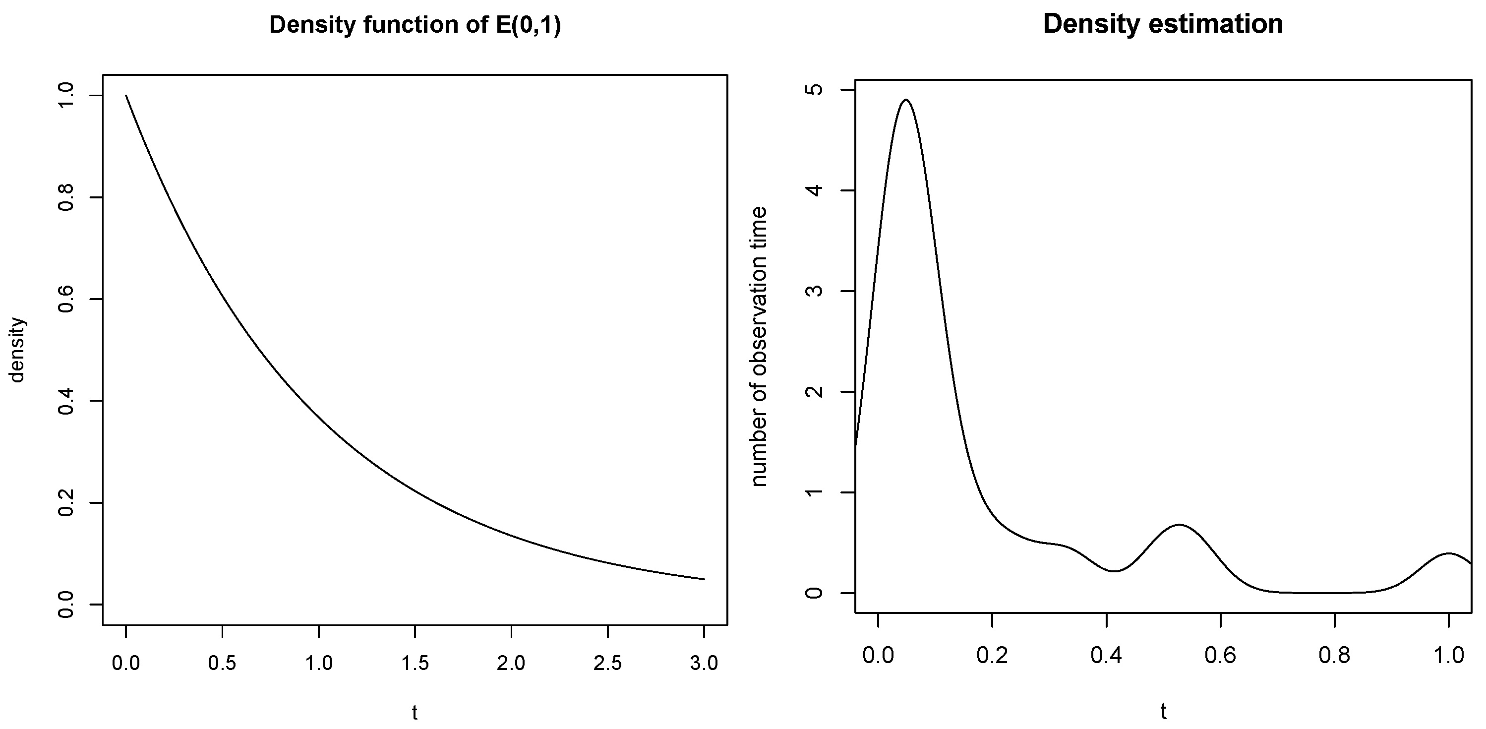
Simulation 1. Assume that the underlying individual curve i at time point $t\in T=[0,1]$ is generated from

$$y_i\left(t\right)={\beta }_0\left(t\right)+{\beta }_1\left(t\right)x_{i1}\left(t\right)+{\beta }_2\left(t\right)x_{i2}\left(t\right)+{ϵ}_i\left(t\right),$$

where ${\beta }_0\left(t\right)\equiv 10,{\beta }_1\left(t\right)=1+t,{\beta }_2\left(t\right)=(1-t)sin\left(2\pi t\right),x_{i1}\left(t\right)=sin\left(100\pi t\right),$$x_{i2}\left(t\right)=cos\left(100\pi t\right)$, and ${ϵ}_i(·)$ is a stationary Gaussian process with zero mean, unit variance, and a constant covariance $0.5$ between any two distinct time points. For each subject i, the number of observation time points $m_i$ is generated from the discrete uniform distribution on $\{5,6,\dots ,30\}$, and the observation time points $t_{ij}$, $j=1,\dots ,m_i$ are independently generated from the exponential distribution $E(0,1)$. The density function of $E(0,1)$ is displayed in the left panel of Figure 1, from which it is easy to see that the density value decreases as t increases.

Figure 1. Left panel visualizes the density function of $E(0,1)$; right panel visualizes the kernel density estimation of the number of observation time of MD001.

Then, we use cubic interpolation to interpolate the $y_i\left(t_{ij}\right)$, $x_{i1}\left(t_{ij}\right)$, and $x_{i2}\left(t_{ij}\right)$ on T to obtain ${\widehat{y}}_i(·)$, ${\widehat{x}}_{i1}(·)$, and ${\widehat{x}}_{i2}(·)$, respectively.

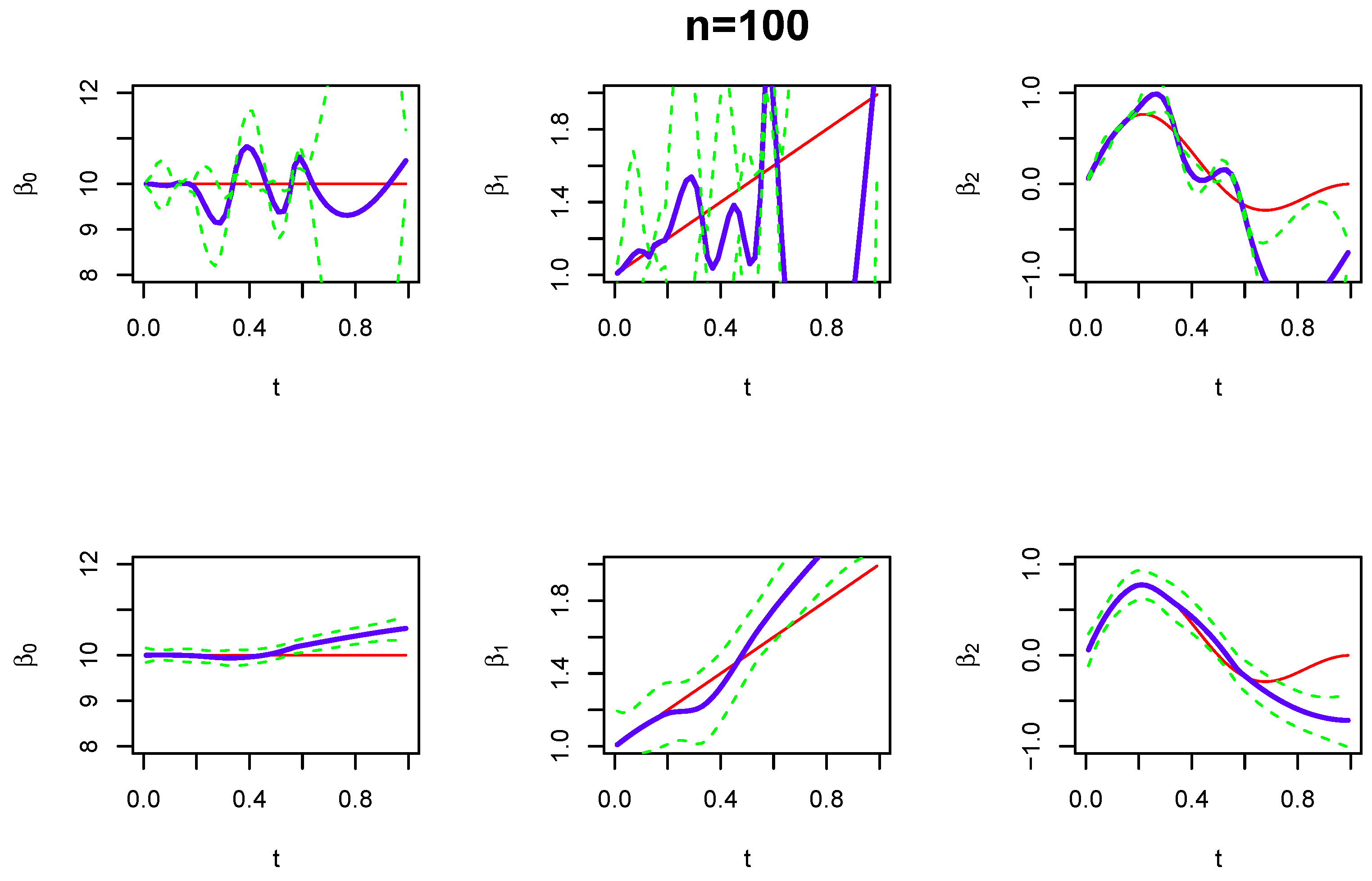
Based on the functions ${\widehat{y}}_i(·)$, ${\widehat{x}}_{i1}(·)$, and ${\widehat{x}}_{i2}(·)$ described above, we use the RKHS introduced in Section 2 to estimate the regression functions ${\beta }_0\left(t\right),{\beta }_1\left(t\right)$, and ${\beta }_2\left(t\right)$, and compare its performance with the spline smoother and local polynomial models. Typical comparisons (the random seed is set to be “set.seed(1)” in R) are given in Figure 2, Figure 3 and Figure 4 with sample sizes of 50, 100, and 200, respectively. The simulation shows that the proposed RKHS method estimates the regression functions well and compares very favorably with the other two methods. Broadly speaking, the RKHS estimator has relatively stable performance and is close to the “true” curve; it has narrower confidence bands at dense sampling regions, and they become wider at sparse sampling regions. On the contrary, the spline smoother and local polynomial model appear to have good fit at dense sampling regions, but they have large bias when the data become sparse.

Figure 2. Performance of curve estimation when the sample size is 50 and the random seed is “set.seed(1)” in R. First row: curve estimation performance of the spline smoother; Second row: curve estimation performance of the local polynomial model; Third row: curve estimation performance of the proposed RKHS method. Solid red line: true curve; Solid blue line: estimated curve; Dotted lower and upper green lines: $95\%$ confidence bands.

Figure 3. Performance of curve estimation when the sample size is 100 and the random seed is “set.seed(1)” in R. First row: curve estimation performance of the spline smoother; Second row: curve estimation performance of the local polynomial model; Third row: curve estimation performance of the proposed RKHS method. Solid red line: true curve; Solid blue line: estimated curve; Dotted lower and upper green lines: $95\%$ confidence bands.

Figure 4. Performance of curve estimation when the sample size is 200 and the random seed is “set.seed(1)” in R. First row: curve estimation performance of the spline smoother; Second row: curve estimation performance of the local polynomial model; Third row: curve estimation performance of the proposed RKHS method. Solid red line: true curve; Solid blue line: estimated curve; Dotted lower and upper green lines: $95\%$ confidence bands.

In order to make a thorough comparison for this simulation, we use the root integrated mean squared prediction error (RIMSPE) to measure the accuracy of the estimates [24]. The RIMSPE for estimate $\widehat{\beta }$ of $\beta$ is given by

$$\mathrm{RIMSPE}\left(\widehat{\beta }\right)=\sqrt{{\int }_0^1{[\beta \left(t\right)-\widehat{\beta }\left(t\right)]}^{2}dt},$$

and the simulation is repeated 1000 times. By using the R software, the CPU time of implementing this simulation is about 84.5 s on a PC with a 1.80 GHz dual-core Intel i5-8265U CPU and 8 GB memory. The boxplots of the RIMSPE values are presented in Figure 5, from which it is clear that RKHS performs much better than the other two methods, because it has much smaller RIMSPE values.

Figure 5. Boxplots of the RIMSPE values. The first row corresponds to sample size 50, the second row corresponds to sample size 100, and the third row corresponds to sample size 200. In each row, the left panel is for estimating ${\beta }_0\left(t\right)$, the middle panel is for estimating ${\beta }_1\left(t\right)$, and the right panel is for estimating ${\beta }_2\left(t\right)$.

Simulation 2. In this simulation study, we examine the performance of Corollary 1 for testing the hypothesis

$$H_0:{\beta }_i\left(t\right)\mathrm{is}\mathrm{linear}\mathrm{in}tVS{H}_1:{\beta }_i\left(t\right)\mathrm{is}\mathrm{not}\mathrm{linear}\mathrm{in}t,\mathrm{for}i=1,2.$$

According to the setting described in Simulation 1, ${\beta }_1\left(t\right)$ is linear in t, whereas ${\beta }_2\left(t\right)$ is apparently not linear in t. Therefore, we will check the type I error for testing ${\beta }_1\left(t\right)$ and the power for testing ${\beta }_2\left(t\right)$. By setting the significance level to $0.05$ and repeating the simulation 1000 times, we use Corollary 1 to derive ${\chi }^2$ testing statistics and list its type I errors and powers in Table 1 for various sample sizes. The results in Table 1 suggest that the type I error of the test is close to the nominal level $0.05$, and the power of the test is not small even with a sample size of 50.

Table 1. Summary of simulation results for linearity testing.

Sample Size	Type I Error (for Testing ${\mathit{\beta }}_0\left(\mathit{t}\right)$)	Power (for Testing ${\mathit{\beta }}_1\left(\mathit{t}\right)$)
50	0.059	0.756
100	0.052	0.865
200	0.051	0.923

The simulation is based on 1000 repetitions.

4. Real Data Analysis

In this section, the proposed method is applied to characterize the relationships in patient immune response in a clinical trial of combination immunotherapy for advanced myeloma. The objective of the original trial was to study whether introducing vaccine-primed T cells early leads to cellular immune responses to the putative tumor antigen hTERT. In this study, 54 patients were recruited and assigned to two treatment arms based on their leukocyte response to human leukocyte antigen A2. Various immune cell parameters (CD3, CD4, CD8), T-cell levels, cytokines (IL7, IL-15), and immunoglobulins (IgA, IgG, IgM) were measured repeatedly to investigate the treatment effect on immune recovery and function. The measurements were taken at nine time points: 0, 2, 7, 14, 40, 60, 90, 100, and 180 days [29]. Moreover, as a subtype of white blood cells in the human immune system, absolute lymphocyte cell (ALC) count was recorded over time during or after patients’ hospitalization up to day 180. Figure 6 shows the trajectories of two individuals, namely “MD001” and “MD002”, in the dataset, with the observation interval scaled to $[0,1]$. The trajectories of all 54 individuals can be found in the paper by Fang et al. [30]. Previous research has shown that the patient’s survival time is associated with the trajectory of the patient’s ALC counts.

Figure 6. Left panel: trajectory of individual “MD001"; right panel: trajectory of individual “MD002". The observation interval has been scaled to $[0,1]$.

In the human immune system, the relationships among various biological features are too complicated and have been topologically described only. For illustrating the performance of our proposed methods with a limited sample size, we only investigate how the levels of a patient’s immunoglobulin IgG and immune cell CD8 dynamically affect the trajectory of the patient’s ALC counts in this section. For simplicity, the observation time points are scaled to the interval $[0,1]$. Let $x_1\left(t\right),x_2\left(t\right)$ and $y\left(t\right)$ be the trajectories of the patient’s IgG, CD8, and ALC counts, respectively. Their relationship can then be described as follows

$$y\left(t\right)={\beta }_0\left(t\right)+{\beta }_1\left(t\right)x_1\left(t\right)+{\beta }_2\left(t\right)x_2\left(t\right)+ϵ\left(t\right),E\left[ϵ\left(t\right)\right]=0,$$

where ${\beta }_0\left(t\right),{\beta }_1\left(t\right)$ and ${\beta }_2\left(t\right)$ are the regression coefficient functions, and $ϵ\left(t\right)$ is the random error function. The purpose of this study is to estimate the regression coefficient functions and test whether ${\beta }_1\left(t\right)$ and ${\beta }_2\left(t\right)$ are linear functions in t.

In the used data, the number of observation times generally becomes sparse as t increases. The right panel of Figure 7 visualizes the kernel density estimation of individual “MD001” in the data. The distribution of observed time points reveals the trend. The proposed RKHS method is used to estimate the regression coefficient functions and test the linearity. By using the R software, the CPU time of implementing the estimation procedure is only about 1.5 s on a PC with a 1.80 GHz dual-core Intel i5-8265U CPU and 8 GB memory. Figure 7 visualizes the estimated curves and their $95\%$ confidence bands. It is observed that ${\beta }_1\left(t\right)$ and ${\beta }_2\left(t\right)$ are apparently nonlinear in t. This observation is also confirmed by the ${\chi }^2$ statistic derived from Corollary 1, which yields p-values less than $0.001$ for both ${\beta }_1\left(t\right)$ and ${\beta }_2\left(t\right)$. It is worth noting that ${\beta }_0\left(t\right)$ is monotone in t, but ${\beta }_1\left(t\right)$ and ${\beta }_2\left(t\right)$ are not monotone in t. The results show that with the immunotherapy of tumor antigen vaccination, a patient’s immunoglobulin IgG enhances the ALC counts. When the increasing CD8 immune cells result in a high ALC count, immunoglobulin IgG inhibits the patient’s ALC counts such that the level of ALC counts is reconverted into the normal interval $(1000,4500)$, and this immunotherapy can potentially improve patient survival time.

Figure 7. The regression coefficient functions estimated by the proposed RKHS method. Solid blue line: estimated curve; dotted lower and upper green lines: $95\%$ confidence bands. The time t has been scaled to the interval $[0,1]$.

5. Concluding Remarks

The existing work on functional data analysis has focused primarily on the case where the observed data are sampled from a dense rate and has been limited to models in which either the response or predictors are functions. In this paper, we consider the more practical situation for functional data analysis where the data are only observed at some (not dense) time points, and we propose a general regression model in which both the response and predictors are functions. This function-on-function regression model, as given by Equation (4), can be viewed as a generalization of multivariate multiple linear regression to allow the response, predictors, and even the regression coefficients to be all functions of t. In order to estimate the underlying regression curves and conduct hypothesis testing on these curves, we use reproducing kernel Hilbert space (RKHS), which only needs to choose the kernel(s) of the RKHS, and enables a closed-form solution for the regression coefficients in terms of the kernel. To the best of our knowledge, this is the first representation of functional regression coefficients with sparsely observed data. Furthermore, the estimator based on RKHS provides a foundation for hypothesis testing, and the asymptotic distribution of the estimator is obtained. Simulation studies show that the RKHS estimator has relatively stable performance. Application and statistical properties of our method are further demonstrated through an immunotherapy clinical trial of advanced myeloma. By using the proposed function-on-function regression model and related theorems established in this paper, this real application showed that with the immunotherapy of tumor antigen vaccination, patient immunoglobulin IgG enhances ALC counts, and hence this immunotherapy can potentially improve patient survival time. Future work may consider experimental design for the time points to be observed. If the time points can be controlled by the experimenter, their careful selection would improve the efficiency of the estimator (e.g., reduce the bias or MES). Further, we hope to study function-on-function generalized linear regressions with sparse estimation coefficient functions by the penalized method of Zhang and Jia [31].