Behavior Analysis of a Class of Discrete-Time Dynamical System with Capture Rate

Abstract

In this paper, we study the stability and bifurcation analysis of a class of discrete-time dynamical system with capture rate. The local stability of the system at equilibrium points are discussed. By using the center manifold theorem and bifurcation theory, the conditions for the existence of flip bifurcation and Hopf bifurcation in the interior of $R_{+}^2$ are proved. The numerical simulations show that the capture rate not only affects the size of the equilibrium points, but also changes the bifurcation phenomenon. It was found that the discrete system not only has flip bifurcation and Hopf bifurcation, but also has chaotic orbital sets. The complexity of dynamic behavior is verified by numerical analysis of bifurcation, phase and maximum Lyapunov exponent diagram.

1. Introduction

The interaction between predator and prey is one of the most popular and interesting research topics for many mathematicians and ecologists. Many researchers have studied the dynamic behavior of prey-predator systems and behavioral phenomena among species in ecology. This also contributes to an increase in the continuous model size of the populations [1,2,3,4,5,6]. In addition, some authors have also studied the complexity, stability, and conditional requirements for the formation of spatial patterns in prey-predator systems [7,8,9,10].

More and more studies show that the discrete-time system is more suitable than the continuous system for small populations, and provides valid proof for this [11,12,13,14,15,16]. In the past few years, many studies have shown that discrete-time predator-prey systems have more abundant dynamic behaviors than continuous systems, such as bifurcation and chaos. They have obtained the relevant dynamic behaviors among populations through numerical simulation [17,18,19,20,21,22,23,24].

Joydip-Dhar et al. [18] studied the following discrete-time prey-predator model with crowding effect and predator partially dependent on prey:

$$\left\{\begin{array}{c}{u}_{n+1}=u_n+\delta [r_1{u}_n(1-\frac{u_n}{k})-\frac{r_2{u}_n{v}_n}{u_n+c}],\hfill \\ v_{n+1}=v_n+\delta (a{v}_n+\frac{r_{2}d{u}_n{v}_n}{u_n+c}-b{v}_n^2),\hfill \end{array}\right.$$

(1)

where $r_1$ and $r_2$ denote the intrinsic growth rates of prey u and predator v populations, respectively, a relates to the growth rate of predator as a result of alternative resources, b indicates competition between individuals due to overcrowding of predator species (i.e., intraspecific interaction), c is the semisaturation constant, d indicates the conversion rate for predator, k is environmental carrying capacity for u, and $\delta$ is the step size.

On the basis of system (1), we introduce the capture rate of predator and prey, and consider the following predator-prey system:

$$\left\{\begin{array}{c}{u}_{n+1}=u_n+\delta [r_1{u}_n(1-\frac{u_n}{k})-\frac{r_2{u}_n{v}_n}{u+c}-h_1{u}_n],\hfill \\ v_{n+1}=v_n+\delta (a{v}_n+\frac{r_{2}d{u}_n{v}_n}{u_n+c}-b{v}_n^2-h_2{v}_n),\hfill \end{array}\right.$$

(2)

where $h_1,h_2$ denote the capture rates of prey and predator, respectively. At the same time, all parameters are greater than zero.

The remainder of the thesis is arranged as follows: In Section 2, the existence and stability of the equilibrium points in interior of $R_{+}^2$ are given. In Section 3, we get the relevant conditions of Hopf bifurcation and flip bifurcation through theoretical analysis. In Section 4, we verify the theoretical results in Section 3 by numerical simulation, and analyze the chaotic phenomenon of discrete system (2). The last section gives a brief conclusion.

2. The Existence and Stability of Fixed Points

In this section, we study the existence and stability of the fixed points by the eigenvalues for the Jacobian matrix corresponding to system (2).

In order to obtain the fixed points of system (2), we calculate the following equations:

$$\left\{\begin{array}{c}u=u+\delta [r_{1}u(1-\frac{u}{k})-\frac{r_{2}uv}{u+c}-h_{1}u],\hfill \\ v=v+\delta (av+\frac{r_{2}duv}{u+c}-b{v}^2-h_{2}v).\hfill \end{array}\right.$$

Through simple calculation, the following results can be obtained directly:

Proposition 1.

$\left(\mathrm{i}\right)$ For all parameter values, (2) has a fixed point $E_1=(0,0)$;

$\left(\mathrm{ii}\right)$ If $r_1>h_1$, then (2) has a boundary equilibrium point $E_2=(\frac{(r_1-h_1)k}{r_1},0)$;

$\left(\mathrm{iii}\right)$ If $a>h_2$, then (2) has a boundary equilibrium point $E_3=(0,\frac{a-h_2}{b})$;

$\left(\mathrm{iv}\right)$ If $a>h_2$, then (2) has a unique positive fixed point $E_4=(u^{*},v^{*})=(u^{*},\frac{1}{b}(a+\frac{d{r}_2{u}^{*}}{u^{*}+c}-h_2))$, where $u^{*}$ is the only positive solution to the cubic equation of one variabie

$$D_0{u}^3+D_1{u}^2+D_{2}u+D_3=0,$$

(3)

where

$D_0=r_{1}bk,D_1=2r_{1}bck-r_{1}b{k}^2-bk{h}_1,$

$D_2=r_{2}ak+r_2^{2}dk-2r_{1}bc{k}^2+r_{1}bk{c}^2-2bck{h}_1-r_{2}k{h}_2,$

$D_3=r_{2}ack-r_{1}b{c}^2{k}^2+b{c}^{2}k{h}_1-r_{2}ck{h}_2$.

The fixed points of system (2) are $E_1(0,0),E_2(\frac{(r_1-h_1)k}{r_1},0),E_3(0,\frac{a-h_2}{b})$ and $E_4(u^{*},v^{*})$, where $u^{*},v^{*}$ satisfy

$$\left\{\begin{array}{c}{r}_1(1-\frac{u^{*}}{k})-\frac{r_2{v}^{*}}{u^{*}+c}-h_1=0,\hfill \\ a+\frac{r_{2}d{u}^{*}}{u^{*}+c}-b{v}^{*}-h_2=0.\hfill \end{array}\right.$$

(4)

The Jacobian matrix corresponding to system (2) at the fixed point $(u,v)$ is as follows

$$A=\left[\begin{array}{cc}1+\delta \left(r_1-\frac{2r_{1}u}{k}-\frac{r_{2}cv}{{(u+c)}^2}-h_1\right)& -\frac{r_2\delta u}{(u+c)}\\ \frac{\delta d{r}_{2}cv}{{(u+c)}^2}& 1+\delta \left(a+\frac{d{r}_{2}u}{u+c}-2bv-h_2\right)\end{array}\right].$$

The characteristic equation of the Jacobian matrix can be written as

$${\lambda }^2+p(u,v)\lambda +q(u,v)=0,$$

(5)

where

$$\begin{array}{cc}\hfill p(u,v)=-trA=& -2-\delta \left(r_1-\frac{2r_{1}u}{k}-\frac{r_{2}cv}{{(u+c)}^2}-h_1+a+\frac{d{r}_{2}u}{u+c}-2bv-h_2\right),\hfill \\ \hfill q(u,v)=detA=& \left[1+\delta \left(r_1-\frac{2r_{1}u}{k}-\frac{r_{2}cv}{{(u+c)}^2}-h_1\right)\right]\left[1+\delta \left(a+\frac{d{r}_{2}u}{u+c}-2bv-h_2\right)\right]+\frac{{\delta }^{2}d{r}_2^{2}cuv}{{(u+c)}^3}.\hfill \end{array}$$

Let ${\lambda }_1$ and ${\lambda }_2$ be two roots of (5), which called eigenvalues of the fixed point $(u,v)$. The fixed point $(u,v)$ is called a sink if $\left|{\lambda }_1\right|<1$ and $\left|{\lambda }_2\right|<1$, the sink is locally asymptotically stable. The fixed point $(u,v)$ is a source if $\left|{\lambda }_1\right|>1$ and $\left|{\lambda }_2\right|>1$, the source is locally unstable. If either $\left|{\lambda }_1\right|=1$ or $\left|{\lambda }_2\right|=1$, then the fixed point $(u,v)$ is non-hyperbolic. The fixed point $(u,v)$ is a saddle if $\left|{\lambda }_1\right|<1$ and $\left|{\lambda }_2\right|>1$ ( or $\left|{\lambda }_1\right|>1$ and $\left|{\lambda }_2\right|<1).$

Proposition 2.

The fixed point $E_2(\frac{(r_1-h_1)k}{r_1},0)$ is a saddle if $0<\delta <\frac{2}{r_1-h_1}$; $E_2(\frac{(r_1-h_1)k}{r_1},0)$ is a source if $\delta >\frac{2}{r_1-h_1}$; and $E_2(\frac{(r_1-h_1)k}{r_1},0)$ is non-hyperbolic if $\delta =\frac{2}{r_1-h_1}.$

Proof. 

For the fixed point $E_2(\frac{(r_1-h_1)k}{r_1},0)$, there is

$$A_{E_2}=\left[\begin{array}{cc}1-\delta \left(r_1-h_1\right)& -\frac{r_2\delta k(r_1-h_1)}{(r_1-h_1)k+r_{1}c}\\ 0& 1+\delta \left(a+\frac{d{r}_{2}k(r_1-h_1)}{(r_1-h_1)k+r_{1}c}-h_2\right)\end{array}\right].$$

The two eigenvalues of the matrix are ${\lambda }_1=1-\delta \left(r_1-h_1\right)$ and ${\lambda }_2=1+\delta \left(a+\frac{d{r}_{2}k(r_1-h_1)}{(r_1-h_1)k+r_{1}c}-h_2\right)$. Apparently ${\lambda }_2$ is greater than 1. When $\left|{\lambda }_1\right|<1$, then $0<\delta <\frac{2}{r_1-h_1}$. Thus, $E_2(\frac{(r_1-h_1)k}{r_1},0)$ is a saddle. On the other side, when $\left|{\lambda }_1\right|>1$, then $\delta >\frac{2}{r_1-h_1}$, $E_2(\frac{(r_1-h_1)k}{r_1},0)$ is a source. When ${\lambda }_1=-1$, then $\delta =\frac{2}{r_1-h_1}$, $E_2(\frac{(r_1-h_1)k}{r_1},0)$ is non-hyperbolic. This completes the proof. □

Proposition 3.

System (2) has the following propositions at the boundary equilibrium point $E_3(0,\frac{a-h_2}{b})$.

$\left(\mathrm{i}\right)\hspace{1em}$$E_3(0,\frac{a-h_2}{b})issinkif{r}_2(a-h_2)+bc{h}_1-r_{1}bc>0and 0<\delta <min\left\{\frac{2}{a-h_2},\frac{2bc}{r_2(a-h_2)+bc{h}_1-r_{1}bc}\right\};$

$\left(\mathrm{ii}\right)\hspace{1em}$$E_3(0,\frac{a-h_2}{b})issourceif{r}_2(a-h_2)+bc{h}_1-r_{1}bc>0and \delta >max\left\{\frac{2}{a-h_2},\frac{2bc}{r_2(a-h_2)+bc{h}_1-r_{1}bc}\right\};$

$\left(\mathrm{iii}\right)\hspace{1em}$$E_3(0,\frac{a-h_2}{b})isnon-hyperbolicif\delta =\frac{2}{a-h_2} or\delta =\frac{2bc}{r_2(a-h_2)+bc{h}_1-r_{1}bc}and r_2(a-h_2)+bc{h}_1-r_{1}bc>0;$

$\left(\mathrm{iv}\right)\hspace{1em}$$E_3(0,\frac{a-h_2}{b})$ is saddle for all values of parameters except those values which lies in (i)–(iii).

Proof. 

(i) For the fixed point $E_3(0,\frac{a-h_2}{b})$, there is

$$A_{E_3}=\left[\begin{array}{cc}1+\delta \left(r_1-\frac{r_2(a-h_2)}{bc}-h_1\right)& 0\\ \frac{\delta d{r}_2(a-h_2)}{bc}& 1-\delta \left(a-h_2\right)\end{array}\right].$$

The two eigenvalues of the matrix are ${\lambda }_1=1+\delta \left(r_1-\frac{r_2(a-h_2)}{bc}-h_1\right)$ and ${\lambda }_2=1-\delta \left(a-h_2\right)$. $E_3(0,\frac{a-h_2}{b})$ is sink if and only if $\left|{\lambda }_1\right|<1$ and $\left|{\lambda }_2\right|<1$.

When $\left|{\lambda }_1\right|<1$, then $0<\delta <\frac{2bc}{r_2(a-h_2)+h_{1}bc-r_{1}bc}$, where $r_2(a-h_2)+h_{1}bc-r_{1}bc>0$. When $\left|{\lambda }_2\right|<1$, then $0<\delta <\frac{2}{a-h_2}$. In conclusion, $E_3(0,\frac{a-h_2}{b})$ is sink if $r_2(a-h_2)+bc{h}_1-r_{1}bc>0$ and $0<\delta <min\left\{\frac{2}{a-h_2},\frac{2bc}{r_2(a-h_2)+bc{h}_1-r_{1}bc}\right\}.$ We can prove (ii), (iii) and (iv) by the same way. This completes the proof. □

Lemma 1

([18]).Let $F\left(\lambda \right)={\lambda }^2+B\lambda +C.$ Suppose that $F\left(1\right)>0$, ${\lambda }_1$ and ${\lambda }_2$ are roots of $F\left(\lambda \right)=0$. Then the following results hold true:

$\left(\mathrm{i}\right)$$\left|{\lambda }_1\right|<1and\left|{\lambda }_2\right|<1ifandonlyif F(-1)>0andC<1;$

$\left(\mathrm{ii}\right)$$\left|{\lambda }_1\right|<1and\left|{\lambda }_2\right|>1(or\left|{\lambda }_1\right|>1and\left|{\lambda }_2\right|<1)ifandonlyifF(-1)<0;$

$\left(\mathrm{iii}\right)$$\left|{\lambda }_1\right|>1and\left|{\lambda }_2\right|>1ifandonlyifF(-1)>0andC>1;$

$\left(\mathrm{iv}\right)$${\lambda }_1=-1and\left|{\lambda }_2\right|\ne 1ifandonlyifF(-1)=0andC\ne 0,2;$

$\left(\mathrm{v}\right)$${\lambda }_{1}and{\lambda }_{2}arecomplexand\left|{\lambda }_1\right|=\left|{\lambda }_2\right|=1ifandonlyif{B}^2-4C<0andC=1.$

Through calculation, we can obtain the characteristic equation of system (2) at the positive equilibrium point $E_4(u^{*},v^{*})$

$${\lambda }^2+p(u^{*},v^{*})\lambda +q(u^{*},v^{*})=0,$$

(6)

where

$p(u^{*},v^{*})=-2-M\delta ,$

$q(u^{*},v^{*})=N{\delta }^2+M\delta +1,$

$M=r_1-\frac{2r_1{u}^{*}}{k}-\frac{r_{2}c{v}^{*}}{{(u^{*}+c)}^2}-h_1+a+\frac{d{r}_2{u}^{*}}{u^{*}+c}-2b{v}^{*}-h_2,$

$N=\left[r_1-\frac{2r_1{u}^{*}}{k}-\frac{r_{2}c{v}^{*}}{{(u^{*}+c)}^2}-h_1\right]\left[a+\frac{d{r}_2{u}^{*}}{u^{*}+c}-2b{v}^{*}-h_2\right]+\frac{d{r}_2^{2}c{u}^{*}{v}^{*}}{{(u^{*}+c)}^3}.$

Now

$$F_{E_4}\left(\lambda \right)={\lambda }^2-(2+M\delta )\lambda +\left(N{\delta }^2+M\delta +1\right).$$

Therefore

$$F\left(1\right)=N{\delta }^2,F(-1)=4+2M\delta +N{\delta }^2.$$

Using Lemma 1, we have the following proposition:

Proposition 4.

System (2) has the following propositions at the positive equilibrium point $E_4(u^{*},v^{*})$.

$\left(\mathrm{i}\right)$$E_4(u^{*},v^{*})isasinkpointifthefollowing(i.1)or(i.2)holds$:

$(\mathrm{i}.1)$$M^2-4N\ge 0and0<\delta <\frac{-M-\sqrt{M^2-4N}}{N},$

$(\mathrm{i}.2)$$M^2-4N<0and0<\delta <\frac{-M}{N}.$

$\left(\mathrm{ii}\right)$$E_4(u^{*},v^{*})issourcepointifthefollowing(ii.1)or(ii.2)holds$:

$(\mathrm{ii}.1)$$M^2-4N\ge 0and\delta >\frac{-M+\sqrt{M^2-4N}}{N},$

$(\mathrm{ii}.2)$$M^2-4N<0and\delta >\frac{-M}{N}.$

$\left(\mathrm{iii}\right)$$E_4(u^{*},v^{*})isnon-hyperbolicifthefollowing(iii.1)or(iii.2)holds$:

$(\mathrm{iii}.1)$$M^2-4N\ge 0and\delta =\frac{-M\pm \sqrt{M^2-4N}}{N},$

$(\mathrm{iii}.2)$$M^2-4N<0and\delta =\frac{-M}{N}.$

$\left(\mathrm{iv}\right)$$E_4(u^{*},v^{*})$ is saddle for all values of parameters except those values which lies in (i) to (iii).

Proof. 

(i) According to Lemma 1, $E_4(u^{*},v^{*})$ is a sink point if and only if $F\left(1\right)>0,F(-1)>0$ and $C<1$, it can be obtained by following calculation.

When $M^2-4N\ge 0$, then $0<\delta <\frac{-M-\sqrt{M^2-4N}}{N};$ and when $M^2-4N<0$, then $0<\delta <\frac{-M}{N}.$ Therefore, Proposition 4 (i) holds. Similarly, Proposition 4 (ii), (iii) and (iv) can be established. □

Through the above analysis, we can get that when the parameters change on sets $F_{E{{}^{\prime }}_4}$ and $F_{E{{}^{″}}_4}$, system (2) will have flip bifurcation at the positive equilibrium point $E_4(u^{*},v^{*})$, where

$$\begin{array}{c}{F}_{E{{}^{\prime }}_4}=\left\{(r_1,r_2,a,b,k,c,d,h_1,h_2,\delta ):\delta =\frac{-M-\sqrt{M^2-4N}}{N},M^2-4N⩾0\right\}.\hfill \end{array}$$

$$\begin{array}{c}{F}_{E{{}^{\prime \prime }}_4}=\left\{(r_1,r_2,a,b,k,c,d,h_1,h_2,\delta ):\delta =\frac{-M+\sqrt{M^2-4N}}{N},M^2-4N⩾0\right\}.\hfill \end{array}$$

When the parameters change on set $F_{E_4}$, system (2) will have Hopf bifurcation at the positive equilibrium point $E_4(u^{*},v^{*})$, where

$$\begin{array}{c}{F}_{E_4}=\left\{(r_1,r_2,a,b,k,c,d,h_1,h_2,\delta ):\delta =-\frac{M}{N},M^2-4N<0\right\}.\hfill \end{array}$$

3. Bifurcation Behavior at ${\mathit{E}}_{\mathbf{4}}({\mathit{u}}^{*},{\mathit{v}}^{*})$

3.1. Flip Bifurcation

We consider the following system

$$\left\{\begin{array}{c}{u}_{n+1}=u_n+{\delta }_1[r_1{u}_n(1-\frac{u_n}{k})-\frac{r_2{u}_n{v}_n}{u+c}-h_1{u}_n],\hfill \\ v_{n+1}=v_n+{\delta }_1(a{v}_n+\frac{r_{2}d{u}_n{v}_n}{u_n+c}-b{v}_n^2-h_2{v}_n),\hfill \end{array}\right.$$

(7)

$(r_1,r_2,a,b,k,c,d,h_1,h_2,{\delta }_1)\in F_{E{{}^{\prime }}_4}$, The eigenvalues of $E_4(u^{*},v^{*})$ are ${\lambda }_1=-1,{\lambda }_2=3+M{\delta }_1$ with $\left|{\lambda }_2\right|\ne 1$ by Proposition 4.

We consider a perturbation of system (7) as follows:

$$\left\{\begin{array}{c}{u}_{n+1}=u_n+({\delta }_1+{\delta }^{*})[r_1{u}_n(1-\frac{u_n}{k})-\frac{r_2{u}_n{v}_n}{u+c}-h_1{u}_n],\hfill \\ v_{n+1}=v_n+({\delta }_1+{\delta }^{*})(a{v}_n+\frac{r_{2}d{u}_n{v}_n}{u_n+c}-b{v}_n^2-h_2{v}_n),\hfill \end{array}\right.$$

(8)

where ${\delta }^{*}$ is a perturbation parameter and $\left|{\delta }^{*}\right|\ll 1$.

Let $w=u-u^{*}$ and $z=v-v^{*}.$ Then we get

$$\left(\begin{array}{c}{w}_{n+1}\\ z_{n+1}\end{array}\right)=\left(\begin{array}{c}{A}_{11}{w}_n+A_{12}{z}_n+A_{13}{w}_n^2+A_{14}{w}_n{z}_n+A_{15}{z}_n^2+B_{11}{\delta }^{*}{w}_n+B_{12}{\delta }^{*}{z}_n\\ +B_{13}{\delta }^{*}{w}_n^2+B_{14}{\delta }^{*}{w}_n{z}_n+B_{15}{\delta }^{*}{z}_n^2+O({\left(|w_n|,|z_n|,\left|{\delta }^{*}\right|\right)}^3)\\ A_{21}{w}_n+A_{22}{z}_n+A_{23}{w}_n^2+A_{24}{w}_n{z}_n+A_{25}{z}_n^2+B_{21}{\delta }^{*}{w}_n+B_{22}{\delta }^{*}{z}_n\\ +B_{23}{\delta }^{*}{w}_n^2+B_{24}{\delta }^{*}{w}_n{z}_n+B_{25}{\delta }^{*}{z}_n^2+O({\left(|w_n|,|z_n|,\left|{\delta }^{*}\right|\right)}^3)\end{array}\right),$$

(9)

where

$$\begin{array}{cc}\hfill A_{11}& =1+{\delta }_1[-\frac{r_1}{k}{u}^{*}+\frac{r_2{u}^{*}{v}^{*}}{{(u^{*}+c)}^2}],A_{12}=-\frac{r_2{\delta }_1{u}^{*}}{u^{*}+c},\hfill \\ \hfill A_{13}& ={\delta }_1[-\frac{r_1}{k}+\frac{r_{2}c{v}^{*}}{{(u^{*}+c)}^3}],A_{14}=-\frac{{\delta }_1{r}_{2}c}{{(u^{*}+c)}^2},\hfill \\ \hfill B_{11}& =-\frac{r_1}{k}{u}^{*}+\frac{r_2{u}^{*}{v}^{*}}{{(u^{*}+c)}^2},B_{12}=-\frac{r_2{u}^{*}}{u^{*}+c},\hfill \\ \hfill B_{13}& =-\frac{r_1}{k}+\frac{r_{2}c{v}^{*}}{{(u^{*}+c)}^3},B_{14}=-\frac{r_{2}c}{{(u^{*}+c)}^2},\hfill \end{array}$$

$$\begin{array}{cc}\hfill A_{21}& =\frac{{\delta }_{1}d{r}_{2}c{v}^{*}}{{(u^{*}+c)}^2},A_{22}=1-{\delta }_{1}b{v}^{*},\hfill \\ \hfill A_{23}& =-\frac{{\delta }_{1}d{r}_{2}c{v}^{*}}{{(u^{*}+c)}^3},A_{24}=\frac{{\delta }_{1}d{r}_{2}c}{{(u^{*}+c)}^2},A_{25}=-{\delta }_{1}b,\hfill \\ \hfill B_{21}& =\frac{d{r}_{2}c{v}^{*}}{{(u^{*}+c)}^2},B_{22}=-b{v}^{*},B_{23}=-\frac{d{r}_{2}c{v}^{*}}{{(u^{*}+c)}^3},\hfill \\ \hfill B_{24}& =\frac{d{r}_{2}c}{{(u^{*}+c)}^2},B_{25}=-b,A_{15}=B_{15}=0.\hfill \end{array}$$

We construct an invertible matrix H and consider the following translation:

$$\left(\begin{array}{c}w\hfill \\ z\hfill \end{array}\right)=H\left(\begin{array}{c}\tilde{u}\hfill \\ \tilde{v}\hfill \end{array}\right),$$

where

$$H=\left(\begin{array}{cc}{A}_{12}& A_{12}\\ -1-A_{11}& {\lambda }_2-A_{11}\end{array}\right).$$

Taking $H^{-1}$ on both sides of system (9), we obtain

$$\left(\begin{array}{c}\tilde{u}\\ \tilde{v}\end{array}\right)=\left(\begin{array}{cc}-1& 0\\ 0& {\lambda }_2\end{array}\right)\left(\begin{array}{c}\tilde{u}\hfill \\ \tilde{v}\hfill \end{array}\right)+\left(\begin{array}{c}f\left(w,z,{\delta }^{*}\right)\hfill \\ g\left(w,z,{\delta }^{*}\right)\hfill \end{array}\right),$$

(10)

where

$$\begin{array}{cc}\hfill f(w,z,{\delta }^{*})& =\frac{[A_{13}({\lambda }_2-A_{11})-A_{12}{A}_{23}]w^2}{A_{12}({\lambda }_2+1)}+\frac{[A_{14}({\lambda }_2-A_{11})-A_{12}{A}_{24}]wz}{A_{12}({\lambda }_2+1)}-\frac{A_{12}{A}_{25}{z}^2}{A_{12}({\lambda }_2+1)}\hfill \\ & +\frac{[B_{11}({\lambda }_2-A_{11})-A_{12}{B}_{21}]{\delta }^{*}w}{A_{12}({\lambda }_2+1)}+\frac{[B_{12}({\lambda }_2-A_{11})-A_{12}{B}_{22}]{\delta }^{*}z}{A_{12}({\lambda }_2+1)}-\frac{A_{12}{B}_{25}{\delta }^{*}{z}^2}{A_{12}({\lambda }_2+1)}\hfill \\ & +\frac{[B_{13}({\lambda }_2-A_{11})-A_{12}{B}_{23}]{\delta }^{*}{w}^2}{A_{12}({\lambda }_2+1)}+\frac{[B_{14}({\lambda }_2-A_{11})-A_{12}{B}_{24}]{\delta }^{*}wz}{A_{12}({\lambda }_2+1)}\hfill \\ & +O\left(\right(\left|w\right|,\left|z\right|,\left|{\delta }^{*}\right|{)}^3),\hfill \end{array}$$

$$\begin{array}{cc}\hfill g(w,z,{\delta }^{*})& =\frac{[A_{13}(1+A_{11})+A_{12}{A}_{23}]w^2}{A_{12}(1+{\lambda }_2)}+\frac{[A_{14}(1+A_{11})+A_{12}{A}_{24}]wz}{A_{12}(1+{\lambda }_2)}+\frac{A_{12}{A}_{25}{z}^2}{A_{12}(1+{\lambda }_2)}\hfill \\ & +\frac{[B_{11}(1+A_{11})+A_{12}{B}_{21}]{\delta }^{*}w}{A_{12}(1+{\lambda }_2)}+\frac{[B_{12}(1+A_{11})+A_{12}{B}_{22}]{\delta }^{*}z}{A_{12}(1+{\lambda }_2)}+\frac{A_{12}{B}_{25}{\delta }^{*}{z}^2}{A_{12}(1+{\lambda }_2)}\hfill \\ & +\frac{[B_{13}(1+A_{11})+A_{12}{B}_{23}]{\delta }^{*}{w}^2}{A_{12}(1+{\lambda }_2)}+\frac{[B_{14}(1+A_{11})+A_{12}{B}_{24}]{\delta }^{*}wz}{A_{12}(1+{\lambda }_2)}\hfill \\ & +O\left(\right(\left|w\right|,\left|z\right|,\left|{\delta }^{*}\right|{)}^3),\hfill \end{array}$$

$$w=A_{12}(\tilde{u}+\tilde{v}),z=({\lambda }_2-A_{11})\tilde{v}-(1+A_{11})\tilde{u}.$$

Applying the center manifold theorem $W^c\left(0\right)$ corresponding to system (10) at the fixed point (0, 0) in a limited neighborhood of ${\delta }^{*}=0.$ The center manifold $W^c\left(0\right)$ can be presented as follows:

$$W^c\left(0\right)=\left\{(\tilde{u},\tilde{v},{\delta }^{*})\in R^3:\tilde{v}(\tilde{u},{\delta }^{*})=A_0{\delta }^{*}+A_1{\tilde{u}}^2+A_2\tilde{u}{\delta }^{*}+A_3{\delta }^{*2}+O\left({\left(|\tilde{u}|+\left|{\delta }^{*}\right|\right)}^3\right)\right\},$$

and satisfy

$$\tilde{H}\left(\tilde{v}(\tilde{u},{\delta }^{*})\right)=\tilde{v}(-\tilde{u}+f(w,\tilde{v}(\tilde{u},{\delta }^{*}),{\delta }^{*}),{\delta }^{*})-{\lambda }_2\tilde{v}(\tilde{u},{\delta }^{*})-g(w,\tilde{v}(\tilde{u},{\delta }^{*}),{\delta }^{*})=0,$$

where $O\left(\right(|\tilde{u}|+\left|{\delta }^{*}\right|{)}^3)$ is an infinitesimal of higher order, and we have

$$\begin{array}{cc}\hfill A_0& =0,\hfill \\ \hfill A_1& =\frac{[A_{13}(1+A_{11})+A_{12}{A}_{23}]A_{12}-[A_{14}(1+A_{11})+A_{12}{A}_{24}](1+A_{11})+A_{25}{(1+A_{11})}^2}{1-{\lambda }_2^2},\hfill \\ \hfill A_2& =\frac{-[B_{11}(1+A_{11})+A_{12}{B}_{21}]A_{12}+[B_{12}(1+A_{11})+A_{12}{B}_{22}](1+A_{11})}{A_{12}{(1+{\lambda }_2)}^2},\hfill \\ \hfill A_3& =0.\hfill \end{array}$$

Therefore, we consider the following mapping:

$$f:\tilde{u}\to -\tilde{u}+n_1{\tilde{u}}^2+n_2\tilde{u}{\delta }^{*}+n_3{\tilde{u}}^2{\delta }^{*}+n_4\tilde{u}{\delta }^{*2}+n_5{\tilde{u}}^3+O\left(\right(|\tilde{u}|+\left|{\delta }^{*}\right|{)}^4),$$

where

$$\begin{array}{cc}\hfill n_1=& \frac{[A_{13}({\lambda }_2-A_{11})-A_{12}{A}_{23}]A_{12}}{1+{\lambda }_2}-\frac{[A_{14}({\lambda }_2-A_{11})-A_{12}{A}_{24}](1+A_{11})}{1+{\lambda }_2}-\frac{A_{12}{A}_{25}{(1+A_{11})}^2}{A_{12}(1+{\lambda }_2)},\hfill \\ \hfill n_2=& \frac{[B_{11}({\lambda }_2-A_{11})-A_{12}{B}_{21}]}{1+{\lambda }_2}-\frac{[B_{12}({\lambda }_2-A_{11})-A_{12}{B}_{22}](1+A_{11})}{A_{12}(1+{\lambda }_2)},\hfill \\ \hfill n_3=& \frac{[A_{13}({\lambda }_2-A_{11})-A_{12}{A}_{23}]2A_2{A}_{12}}{1+{\lambda }_2}+\frac{[A_{14}({\lambda }_2-A_{11})-A_{12}{A}_{24}]({\lambda }_2-2A_{11}-1)A_2}{1+{\lambda }_2}\hfill \\ & -\frac{B_{25}{(1+A_{11})}^2}{1+{\lambda }_2}+\frac{2A_{25}(1+A_{11})({\lambda }_2-A_{11})A_2}{1+{\lambda }_2}+\frac{[B_{11}({\lambda }_2-A_{11})-A_{12}{B}_{21}]A_1}{1+{\lambda }_2}\hfill \\ & +\frac{[B_{13}({\lambda }_2-A_{11})-A_{12}{B}_{23}]A_{12}}{1+{\lambda }_2}-\frac{[B_{14}({\lambda }_2-A_{11})-A_{12}{B}_{24}](1+A_{11})}{1+{\lambda }_2}\hfill \\ & +\frac{[B_{12}({\lambda }_2-A_{11})-A_{12}{B}_{22}]({\lambda }_2-A_{11})A_1}{A_{12}(1+{\lambda }_2)},\hfill \\ \hfill n_4=& \frac{[B_{11}({\lambda }_2-A_{11})-A_{12}{B}_{21}]A_2}{1+{\lambda }_2}+\frac{[B_{12}({\lambda }_2-A_{11})-A_{12}{B}_{22}]({\lambda }_2-A_{11})A_2}{A_{12}({\lambda }_2+1)},\hfill \\ \hfill n_5=& \frac{[A_{13}({\lambda }_2-A_{11})-A_{12}{A}_{23}]2A_{12}{A}_1}{1+{\lambda }_2}+\frac{[A_{14}({\lambda }_2-A_{11})-A_{12}{A}_{24}]({\lambda }_2-2A_{11}-1)A_1}{{\lambda }_2+1}\hfill \\ & +\frac{2A_{25}(1+A_{11})({\lambda }_2-A_{11})A_1}{1+{\lambda }_2}.\hfill \end{array}$$

According to flip bifurcation, we require that two discriminatory quantities ${\tau }_1$ and ${\tau }_2$ are not zero, where

$${\tau }_1={\left.\left(\frac{{\partial }^{2}f}{\partial \tilde{u}\partial {\delta }^{*}}+\frac{1}{2}\frac{\partial f}{\partial {\delta }^{*}}\frac{{\partial }^{2}f}{\partial {\tilde{u}}^2}\right)\right|}_{(0,0)},{\tau }_2={\left.\left(\frac{1}{6}\frac{{\partial }^{3}f}{\partial {\tilde{u}}^3}+{\left(\frac{1}{2}\frac{{\partial }^{2}f}{\partial {\tilde{u}}^2}\right)}^2\right)\right|}_{(0,0)}.$$

By simple calculations, we obtain ${\tau }_1=n_2$ and ${\tau }_2=n_1^2+n_5.$

From the above analysis, we have the following theorem:

Theorem 1.

If ${\tau }_1\ne 0,{\tau }_2\ne 0$, then system (8) passes through a flip bifurcation at the fixed point $E_4(u^{*},v^{*})$ when the parameter ${\delta }^{*}$ alters in the small region of the point (0, 0). In addition, if ${\tau }_2>0$ (resp., ${\tau }_2<0$), then the period-2 points that bifurcate from fixed point $E_4(u^{*},v^{*})$ are stable (resp., unstable).

3.2. Hopf Bifurcation

We consider a perturbation of system (2) as follows:

$$\left\{\begin{array}{c}{u}_{n+1}=u_n+({\delta }_2+\delta )[r_1{u}_n(1-\frac{u_n}{k})-\frac{r_2{u}_n{v}_n}{u_n+c}-h_1{u}_n],\hfill \\ v_{n+1}=v_n+({\delta }_2+\delta )[a{v}_n+\frac{r_{2}d{u}_n{v}_n}{u_n+c}-b{v}_n^2-h_2{v}_n],\hfill \end{array}\right.$$

(11)

where $\delta$ is a perturbation parameter and $\left|\delta \right|\ll 1$.

The characteristic equation of system (11) at the positive equilibrium point $E_4(u^{*},v^{*})$ is as follows:

$${\lambda }^2+p\left(\delta \right)\lambda +q\left(\delta \right)=0,$$

where

$p\left(\delta \right)=-2-M(\delta +{\delta }_2),q\left(\delta \right)=N{(\delta +{\delta }_2)}^2+M(\delta +{\delta }_2)+1.$

When parameters $(r_1,r_2,a,b,k,c,d,h_1,h_2,{\delta }_2)\in F_{E_4}$, the characteristic values of system (11) at the positive equilibrium point $E_4(u^{*},v^{*})$ are as follows:

$$\lambda ,\overline{\lambda }=\frac{-p\left(\delta \right)\pm i\sqrt{4q\left(\delta \right)-p^2\left(\delta \right)}}{2}.$$

Therefore

$$\lambda ,\overline{\lambda }=1+\frac{M({\delta }_2+\delta )}{2}\pm \frac{i({\delta }_2+\delta )\sqrt{4N-M^2}}{2},$$

and we have

$$\left|\lambda \right|=|\overline{\lambda }{|=\left(q\left(\delta \right)\right)}^{1/2},l={\left.\frac{d\left|\lambda \right|}{d\delta }\right|}_{\delta =0}={\left.\frac{d|\overline{\lambda }|}{d\delta }\right|}_{\delta =0}=-\frac{M}{2}>0.$$

When $\delta$ changes in limited neighborhood of $\delta =0,$ then $\lambda ,\overline{\lambda }=\alpha \pm i\beta ,$ where

$$\alpha =1+\frac{{\delta }_{2}M}{2},\beta =\frac{{\delta }_2\sqrt{4N-M^2}}{2}.$$

In addition, Hopf bifurcation requires that $\delta =0$, ${\lambda }^m,{\overline{\lambda }}^m\ne 1$ (m = 1, 2, 3, 4) which is equivalent to $p\left(0\right)\ne$−2, 0, 1, 2. Because parameter $(r_1,r_2,a,b,k,c,d,h_1,h_2,{\delta }_2)\in F_{E_4}$, therefore $p\left(0\right)\ne$ −2, 2. We only require $p\left(0\right)\ne$ 0, 1, so that

$$\begin{array}{c}\hfill M^2\ne 2N,3N.\end{array}$$

(12)

Let $w=u-u^{*}$ and $z=v-v^{*}.$ Then we get

$$\left(\begin{array}{c}{w}_{n+1}\\ z_{n+1}\end{array}\right)=\left(\begin{array}{c}{A}_{11}{w}_n+A_{12}{z}_n+A_{13}{w}_n^2+A_{14}{w}_n{z}_n+A_{15}{z}_n^2+O({\left(|w_n|,|z_n|\right)}^3)\\ A_{21}{w}_n+A_{22}{z}_n+A_{23}{w}_n^2+A_{24}{w}_n{z}_n+A_{25}{z}_n^2+O({\left(|w_n|,|z_n|\right)}^3)\end{array}\right),$$

(13)

where $A_{11},A_{12},A_{13},A_{14},A_{15},A_{21},A_{22},A_{23},A_{24},A_{25}$ are given in (9) by substituting ${\delta }_2$ for ${\delta }_2+\delta$.

Next, we discuss the normal form corresponding to system (13) when $\delta =0.$

Consider the translation as follows:

$$\left(\begin{array}{c}w\hfill \\ z\hfill \end{array}\right)=H\left(\begin{array}{c}\tilde{u}\hfill \\ \tilde{v}\hfill \end{array}\right),$$

where

$$H=\left(\begin{array}{cc}{A}_{12}& 0\\ \alpha -A_{11}& -\beta \end{array}\right).$$

Taking $H^{-1}$ on both sides of system (13), we obtain

$$\left(\begin{array}{c}\tilde{u}\\ \tilde{v}\end{array}\right)=\left(\begin{array}{cc}\alpha & -\beta \\ \beta & \alpha \end{array}\right)\left(\begin{array}{c}\tilde{u}\hfill \\ \tilde{v}\hfill \end{array}\right)+\left(\begin{array}{c}\tilde{f}\left(\tilde{u},\tilde{v}\right)\hfill \\ \tilde{g}\left(\tilde{u},\tilde{v}\right)\hfill \end{array}\right),$$

where

$$\begin{array}{cc}& \tilde{f}(\tilde{u},\tilde{v})=\frac{A_{13}{w}^2}{A_{12}}+\frac{A_{14}wz}{A_{12}}+{O\left(\right(\left|w\right|,\left|z\right|)}^3),\hfill \\ & \tilde{g}(\tilde{u},\tilde{v})=\frac{[A_{13}(\alpha -A_{11})-A_{12}{A}_{23}]w^2}{A_{12}\beta }+\frac{[A_{14}(\alpha -A_{11})-A_{12}{A}_{24}]wz}{A_{12}\beta }-\frac{A_{25}{z}^2}{\beta }+{O\left(\right(\left|w\right|,\left|z\right|)}^3),\hfill \\ & w=A_{12}\tilde{u},\hfill \\ & z=(\alpha -A_{11})\tilde{u}-\beta \tilde{v}.\hfill \end{array}$$

Hence

$$\begin{array}{c}{\tilde{f}}_{\overline{u}\overline{u}}=2A_{12}{A}_{13}+2A_{14}(\alpha -A_{11}),{\tilde{f}}_{\overline{u}\overline{v}}=-A_{14}\beta ,{\tilde{f}}_{\overline{v}\overline{v}}=0,\hfill \\ {\tilde{f}}_{\overline{u}\overline{u}\overline{u}}=0,{\tilde{f}}_{\overline{u}\overline{u}\overline{v}}=0,{\tilde{f}}_{\overline{u}\overline{v}\overline{v}}=0,{\tilde{f}}_{\overline{v}\overline{v}\overline{v}}=0,\hfill \\ {\tilde{g}}_{\overline{u}\overline{u}}=\frac{2A_{12}}{\beta }[A_{13}(\alpha -A_{11})-A_{12}{A}_{23}]+\frac{2(\alpha -A_{11})}{\beta }[A_{14}(\alpha -A_{11})-A_{12}{A}_{24}]-\frac{2A_{25}}{\beta }{(\alpha -A_{11})}^2,\hfill \\ {\tilde{g}}_{\overline{u}\overline{v}}=-[A_{14}(\alpha -A_{11})-A_{12}{A}_{24}]+2A_{25}(\alpha -A_{11}),{\tilde{g}}_{\overline{v}\overline{v}}=-2A_{25}\beta ,\hfill \\ {\tilde{g}}_{\overline{u}\overline{u}\overline{u}}=0,{\tilde{g}}_{\overline{u}\overline{u}\overline{v}}=0,{\tilde{g}}_{\overline{u}\overline{v}\overline{v}}=0,{\tilde{g}}_{\overline{v}\overline{v}\overline{v}}=0.\hfill \end{array}$$

System (2) undergoes the Hopf bifurcation if the following quantity is not zero

$$L=-Re\left[\frac{(1-2\overline{\lambda }){\overline{\lambda }}^2}{1-\lambda }{\omega }_{11}{\omega }_{20}\right]-\frac{1}{2}{∥{\omega }_{11}∥}^2-{∥{\omega }_{02}∥}^2+Re\left(\overline{\lambda }{\omega }_{21}\right),$$

(14)

where

$$\begin{array}{cc}\hfill {\omega }_{20}& =\frac{1}{8}[({\tilde{f}}_{\overline{u}\overline{u}}-{\tilde{f}}_{\overline{v}\overline{v}}+2{\tilde{g}}_{\overline{u}\overline{v}})+i({\tilde{g}}_{\overline{u}\overline{u}}-{\tilde{g}}_{\overline{v}\overline{v}}-2{\tilde{f}}_{\overline{u}\overline{v}})],\hfill \\ \hfill {\omega }_{11}& =\frac{1}{4}[({\tilde{f}}_{\overline{u}\overline{u}}+{\tilde{f}}_{\overline{v}\overline{v}})+i({\tilde{g}}_{\overline{u}\overline{u}}+{\tilde{g}}_{\overline{v}\overline{v}})],\hfill \\ \hfill {\omega }_{02}& =\frac{1}{8}[({\tilde{f}}_{\overline{u}\overline{u}}-{\tilde{f}}_{\overline{v}\overline{v}}-2{\tilde{g}}_{\overline{u}\overline{v}})+i({\tilde{g}}_{\overline{u}\overline{u}}-{\tilde{g}}_{\overline{v}\overline{v}}+2{\tilde{f}}_{\overline{u}\overline{v}})],\hfill \\ \hfill {\omega }_{21}& =\frac{1}{16}[({\tilde{f}}_{\overline{u}\overline{u}\overline{u}}+{\tilde{f}}_{\overline{u}\overline{v}\overline{v}}+{\tilde{g}}_{\overline{u}\overline{u}\overline{v}}+{\tilde{g}}_{\overline{v}\overline{v}\overline{v}})+i({\tilde{g}}_{\overline{u}\overline{u}\overline{u}}+{\tilde{g}}_{\overline{u}\overline{v}\overline{v}}-{\tilde{f}}_{\overline{u}\overline{u}\overline{v}}-{\tilde{f}}_{\overline{v}\overline{v}\overline{v}})].\hfill \end{array}$$

If $L\ne 0$, Hopf bifurcation will occur in system (2), and we have the following theorem holds:

Theorem 2.

If the condition (12) holds, and $L\ne 0$, then system (11) passes through a Hopf bifurcation at the fixed point $E_4(u^{*},v^{*})$ when the parameter δ alters in the small region of the point (0, 0). In addition, if $L>0$ (resp., $L<0$), then an repelling (resp., attracting) invariant closed curve bifurcates from fixed point $E_4(u^{*},v^{*})$ for $\delta <0$ (resp., $\delta >0$).

4. Numerical Simulations

In this section, we will verify the previous theoretical results through numerical simulation. By drawing bifurcation diagram, phase diagram and maximum Lyapunov exponent diagram, the dynamic behavior of discrete system (2) is analyzed and summarized. The bifurcation behavior of system (2) is considered in the following cases:

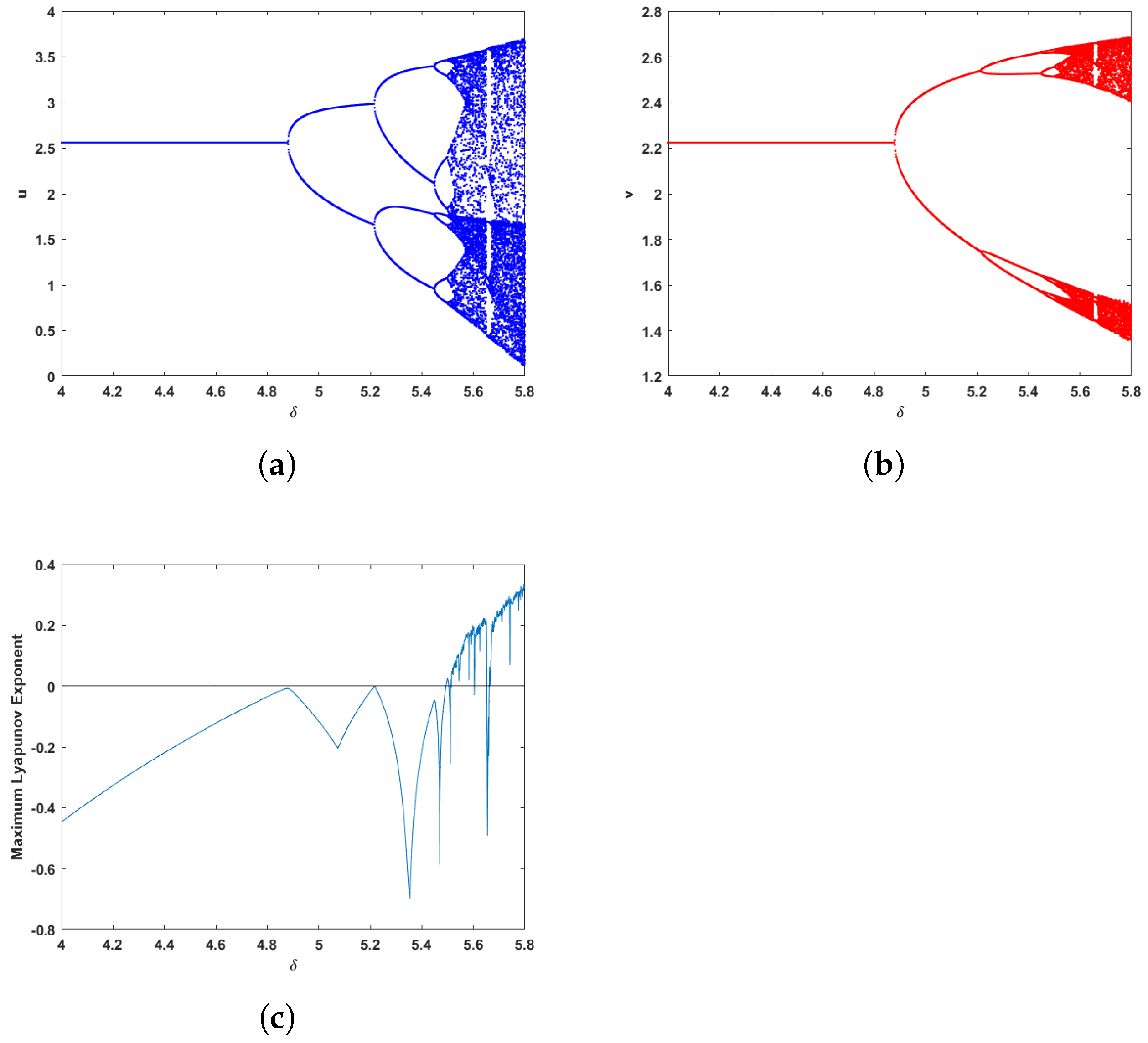
Firstly, in Figure 1, we consider that the capture rates of prey and predator $h_1=h_2=0$ and take $\delta$ as the bifurcation parameter to analyze the dynamic behavior of system (2) at the positive equilibrium point. We consider the parameter values as $(r_1,r_2,a,b,c,d,k,h_1,h_2)=(0.8,0.8,0.4,0.2,2,0.1,5,0,0)\in F_{E{{}^{\prime }}_4}$ with the initial value of $(u,v)$ = (3, 2) and $\delta \in$ [4, 5.8]. A flip bifurcation (period-doubling bifurcation) emerges from the fixed point (2.56155, 2.22462) at $\delta =4.87985,$ and it is stable when $\delta <4.87985$, and when $\delta >4.87985$, system (2) oscillates with periods of $2,4,8,\cdots .$ It can be obtained from Figure 1c that chaos will occur in system (2) as the bifurcation parameters $\delta$ continue to increase.

Figure 1. (a,b) Bifurcation diagram corresponding to u and v in system (2) with $\delta \in$ [4, 5.8], $r_1=0.8, r_2=0.8, a=0.4, b=0.2, c=2, d=0.1, k=5, h_1=h_2=0,$ the initial value is $(u,v)$ = (3, 2). (c) Maximum Lyapunov exponents corresponding to (a).

In Figure 2, we consider that the capture rates of prey and predator $h_1=0,h_2=0.1$, respectively. Taking $(r_1,r_2,a,b,c,d,k,h_1,h_2)=(0.8,0.8,0.4,0.2,2,0.1,5,0,0.1)\in F_{E_4}$ with the initial value of $(u,v)$ = (3, 2) and $\delta \in$ [5, 6.2]. Hopf bifurcation emerges from the fixed point (3.36948, 1.7510) at $\delta =5.3218$ with $\alpha$ = −0.9308, $\beta$ = 0.3656. It verifies that Theorem 2 holds.

Figure 2. (a,b) Bifurcation diagram corresponding to u and v in system (2) with $\delta \in$ [5, 6.2], $r_1=0.8, r_2=0.8, a=0.4, b=0.2, c=2, d=0.1, k=5, h_1=0, h_2=0.1,$ the initial value is $(u,v)$ = (3, 2). (c) Maximum Lyapunov exponents related to (a).

In Figure 3, we can observe that the equilibrium point (3.36948, 1.7510) of system (2) is stable for $\delta <5.3218$, loses its stability at $\delta =5.3218$ and not only a limit cycle but also periodic solution appear when the bifurcation parameter $\delta >5.3218$. Furthermore, the value of the maximum Lyapunov exponents related to system (2) is greater than 0 as $\delta$ continues to increase, and thus chaos will occur, i.e., the solution of system (2) is arbitrarily periodic. At the same time, if only the predator is properly captured, its population density decreases, and the prey population density increases. Compared with Figure 1, the bifurcation at the positive equilibrium point also changes from flip bifurcation to Hopf bifurcation.

Figure 3. Phase portraits and solution portraits for various values of $\delta$ corresponding to Figure 2a. (a) $\delta =5.2$. (b) $\delta =5.4$. (c) $\delta =6$. (d) solution portrait for $\delta =5.2$. (e) solution portrait for $\delta =5.4$. (f) solution portrait for $\delta =6$.

In Figure 4, we consider that the capture rates of prey and predator $h_1=0.06,h_2=0$, respectively. Taking $(r_1,r_2,a,b,c,d,k,h_1,h_2)=(0.8,0.8,0.4,0.2,2,0.1,5,0.06,0)\in F_{E{{}^{\prime }}_4}$ with the initial value of $(u,v)$ = (3, 2) and $\delta \in$ [4, 6.5]. A flip bifurcation (period-doubling bifurcation) emerges from the equilibrium point (1.6013, 2.1779) at $\delta =4.8821,$ and it is stable when $\delta <4.8821$ and when $\delta >4.8821$, system (2) oscillates with periods of $2,4,8,\cdots .$ It can be obtained from Figure 4b that chaos will occur in system (2) as the bifurcation parameters $\delta$ continue to increase. At the same time, if only the prey is properly captured, its population density decreases, and the predator population density decreases. Compared with Figure 1, the bifurcation at the positive equilibrium point does not change.

Figure 4. (a,b) Bifurcation diagram corresponding to u and v in system (2) with $\delta \in$ [4, 6.5], $r_1=0.8, r_2=0.8, a=0.4, b=0.2, c=2, d=0.1, k=5, h_1=0.06, h_2=0,$ the initial value is $(u,v)$ = (3, 2). (c) Maximum Lyapunov exponents related to (a).

In Figure 5, we consider that the capture rates of prey and predator $h_1=0.1,h_2=0.1$, respectively. Taking $(r_1,r_2,a,b,c,d,k,h_1,h_2)=(0.8,0.8,0.4,0.2,2,0.1,5,0.1,0.1)\in F_{E_4}$ with the initial value of $(u,v)$ = (3, 2) and $\delta \in$ [6.4, 7.4]. Hopf bifurcation emerges from the fixed point (2.4372, 1.7197) at $\delta =6.8995$ with $\alpha$ = −0.3751, $\beta$ = 0.2329.

Figure 5. (a,b) Bifurcation diagram corresponding to u and v in system (2) with $\delta \in$ [6.4, 7.4], $r_1=0.8, r_2=0.8, a=0.4, b=0.2, c=2, d=0.1, k=5, h_1=0.1, h_2=0.1,$ the initial value is $(u,v)$ = (3, 2).

In Figure 6, we can observe that the equilibrium point (2.4372, 1.7197) of system (2) is stable for $\delta <6.8995$, loses its stability at $\delta =6.8995$ and not only an invariant circle but also periodic solution appear when the bifurcation parameter $\delta >6.8995$. The phase diagrams in Figure 6 indicate that a smooth limit cycle bifurcates from the positive equilibrium point and its radius increases as $\delta$ increases. When $h_1=0.1,h_2=0.1$, system (2) changes from flip bifurcation to Hopf bifurcation, and will produce chaos as $\delta$ increases. Furthermore, when $h_1=0.1,h_2=0.1$, system (2) will occur not only Hopf bifurcation and chaos, but also the equilibrium point be lowered. Compared with Figure 1, the bifurcation at the positive equilibrium point also changes from flip bifurcation to Hopf bifurcation. So it can be concluded that the capture effect has a great effect on the dynamic behavior of system (2).

Figure 6. Phase portraits and solution portraits for various values of $\delta$ corresponding to Figure 5a. (a) $\delta =6.8$. (b) $\delta =6.94$. (c) $\delta =7.1$. (d) solution portrait for $\delta =6.8$. (e) solution portrait for $\delta =6.94$. (f) solution portrait for $\delta =7.1$.

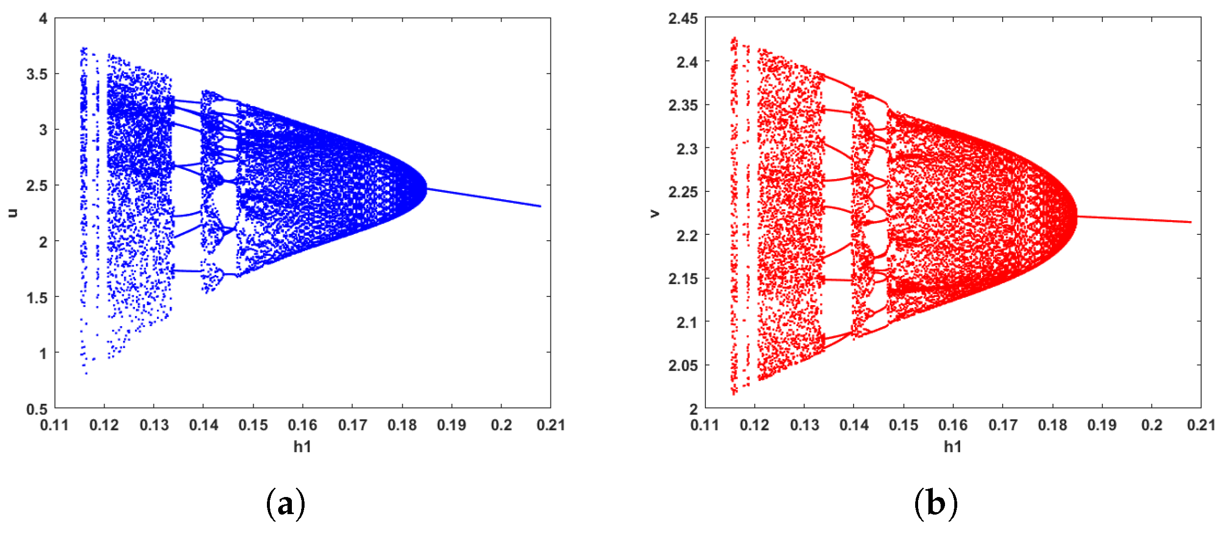
In Figure 7, when the parameter value is $(r_1,r_2,a,b,c,d,k,\delta ,h_2)$ = (1.15, 0.8, 0.4, 0.2, 2, 0.1, 5, 4.88, 0) with the initial value of $(u,v)$ = (4, 2) and $h_1\in$ [0.11, 0.21], $h_1$ is bifurcation parameter. Figure 7 shows the occurrence of Hopf bifurcation, the bifurcation graph fist appears chaos, then orbital lines and periodic solutions, and finally tends to be stable as the value of parameter $h_1$ increases. In addition, the population density of prey and predator will decrease with the increasing of prey capture rate $h_1$.

Figure 7. Bifurcation diagram of system (2) with $h_1\in$ [0.11, 0.21], $r_1=1.15, r_2=0.8, a=0.4, b=0.2, c=2, d=0.1, k=5, \delta =4.88, h_2=0,$ the initial value is $(u,v)$ = (4, 2). (a) Bifurcation diagram for u. (b) Bifurcation diagram for v.

In Figure 8, when the parameter value is $(r_1,r_2,a,b,c,d,k,\delta ,h_1)$ = (0.8, 0.8, 0.4, 0.2, 2, 0.1, 5, 4.88, 0) with the initial value of $(u,v)$ = (4, 2) and $h_2\in$ [0, 0.25], $h_2$ is bifurcation parameter. It can be seen from Figure 8 that as the parameter value $h_2$ continues to increase, the flip bifurcation will occur. In addition, the population density of prey and predator will increase and decrease with the increasing of predator capture rate $h_2$.

Figure 8. Bifurcation diagram of system (2) with $h_2\in$ [0, 0.25], $r_1=0.8, r_2=0.8, a=0.4, b=0.2, c=2, d=0.1, k=5, h_1=0, \delta =4.88,$ the initial value is $(u,v)$ = (4, 2). (a) Bifurcation diagram for u. (b) Bifurcation diagram for v.

5. Conclusions

Research indicates that the discrete systems compared to the continuous systems have richer and more complex dynamic behaviors. Therefore, on the basis of previous study work, this paper studies the stability and bifurcation analysis of a class of discrete-time dynamical system with capture rate in the closed first quadrant $R_{+}^2$. According to the research results, we can obtain the following results:

(1) System (2) has four fixed points, in which the stable fixed point is positive, reflecting the stable coexistence of prey and predators.

(2) System (2) has flip bifurcation at the boundary equilibrium point, flip bifurcation and Hopf bifurcation occur at the positive equilibrium point when $\delta$ changes in $F_{E{{}^{\prime }}_4}$ or $F_{E{{}^{″}}_4}$ and $F_{E_4}$ small fields. It can be seen from Figure 1 and Figure 2 that the flip bifurcation and Hopf bifurcation at the positive equilibrium point will produce chaos. We can also find the orbits of periods 2, 4, and 8 periodic windows of flip bifurcation.

(3) When $h_1=0,h_2\ne 0$, the equilibrium point of system (2) changes compared to system (1), where $u^{*}$ goes up and $v^{*}$ goes down. The number of predators goes up and the number of prey goes up. In addition, under the same set of parameters, flip bifurcation occurs in system (1) and Hopf bifurcation occurs in system (2), thus the bifurcation phenomenon changes (see Figure 1 and Figure 2).

(4) When $h_1\ne 0,h_2=0$, the equilibrium point of system (2) changes compared to system (1), where $u^{*}$ and $v^{*}$ both go down. The number of predators and prey go down. In addition, under the same set of parameters, the bifurcation of system (2) at the positive equilibrium point does not change compared to system (1) (see Figure 1 and Figure 4).

(5) When $h_1\ne 0,h_2\ne 0$, the equilibrium point of system (2) changes compared to system (1), where $u^{*}$ and $v^{*}$ both go down. The density of both predators and prey populations decreased. In addition, under the same set of parameters, the bifurcation of system (2) at the positive equilibrium point change from flip bifurcation to Hopf bifurcation compared to system (1) (see Figure 1 and Figure 5).