Remarks on the Vertex and the Edge Metric Dimension of 2-Connected Graphs

Abstract

The vertex (respectively edge) metric dimension of a graph G is the size of a smallest vertex set in G, which distinguishes all pairs of vertices (respectively edges) in G, and it is denoted by $\dim \left(G\right)$ (respectively $\mathrm{edim}\left(G\right)$). The upper bounds $\dim \left(G\right)\le 2c\left(G\right)-1$ and $\mathrm{edim}\left(G\right)\le 2c\left(G\right)-1,$ where $c\left(G\right)$ denotes the cyclomatic number of G, were established to hold for cacti without leaves distinct from cycles, and moreover, all leafless cacti that attain the bounds were characterized. It was further conjectured that the same bounds hold for general connected graphs without leaves, and this conjecture was supported by showing that the problem reduces to 2-connected graphs. In this paper, we focus on $\Theta$-graphs, as the most simple 2-connected graphs distinct from the cycle, and show that the the upper bound $2c\left(G\right)-1$ holds for both metric dimensions of $\Theta$-graphs; we characterize all $\Theta$-graphs for which the bound is attained. We conclude by conjecturing that there are no other extremal graphs for the bound $2c\left(G\right)-1$ in the class of leafless graphs besides already known extremal cacti and extremal $\Theta$-graphs mentioned here.

1. Introduction

In this paper, we assume that all graphs are simple and connected, unless we explicitly say otherwise, and we consider distances in such graphs. Let G be a graph with the set of vertices $V\left(G\right)$ and the set of edges $E\left(G\right).$ The distance $d_G(u,v)$ between vertices $u,v\in V\left(G\right)$ is the length of a shortest path in G connecting vertices u and $v.$ The distance $d_G(u,e)$ between a vertex $u\in V\left(G\right)$ and an edge $e=vw\in E\left(G\right)$ is defined by $d_G(u,e)=min\{d_G(u,v),d_G(u,w)\}.$ When no confusion arises from that, we use abbreviated notation $d(u,v)$ and $d(u,e).$ We say that a pair x and $x^{\prime }$ of vertices from $V\left(G\right)$ (respectively of edges from $E\left(G\right)$) is distinguished by a vertex $s\in V\left(G\right)$ if $d(s,x)\ne d(s,x^{\prime })$. A set S is a vertex (respectively an edge) metric generator if every pair x and $x^{\prime }$ of vertices from $V\left(G\right)$ (respectively of edges from $E\left(G\right)$) is distinguished by a vertex $s\in S.$ The size of a smallest vertex (respectively edge) metric generator in G is called the vertex (respectively the edge) metric dimension of G, and it is denoted by $\dim \left(G\right)$ (respectively $\mathrm{edim}\left(G\right)$). The cyclomatic number $c\left(G\right)$ of a graph G is defined by $c\left(G\right)=\left|E\left(G\right)\right|-\left|V\left(G\right)\right|+1.$ A $\Theta$-graphis any graph G with precisely two vertices of degree 3 and all other vertices of degree 2.

The concept of the vertex metric dimension was introduced related to the study of navigation systems [1] and the landmarks in networks [2]. Various aspects of this metric dimension have been studied since it was first introduced [3,4,5,6,7,8,9,10]. As was noticed recently in [11], there are graphs in which none of the smallest vertex metric generators distinguish all pairs of edges. This motivated the introduction of a new variant of the metric dimension, namely the edge metric dimension. Even though it is newer than the vertex metric dimension, the edge metric dimension also attracted interest [12,13,14,15,16,17,18,19,20]. A nice survey of the topic of the metric dimension is given in [21].

Particularly relevant for this paper is the line of investigation from papers [17,22,23,24,25,26]. In [22], the value of the vertex and edge metric dimensions for unicyclic graphs was bounded so it can take only two consecutive integer values, and then, in [17], the condition under which the dimensions take each of the values was established. This result was further extended to graphs with edge disjoint cycles [25], also called cactus graphs or cacti. A similar line of research for another variant of the metric dimension, the so-called mixed metric dimension, was conducted in [23,24,27]. The results for cacti from [25] imply that the simple upper bounds $\dim \left(G\right)\le L\left(G\right)+2c\left(G\right)$ and $\mathrm{edim}\left(G\right)\le L\left(G\right)+2c\left(G\right)$ hold for all cacti G distinct from paths, where

$$L\left(G\right)=\sum _{v\in V\left(G\right),\ell \left(v\right)>1}(\ell \left(v\right)-1),$$

with $\ell \left(v\right)$ being the number of paths pending at a vertex v of degree $\ge 3.$ Moreover, the following conjectures were proposed for general graphs.

Moreover, the following conjectures were proposed for general graphs.

Conjecture 1.

Let G be a connected graph. Then, $\dim \left(G\right)\le L\left(G\right)+2c\left(G\right).$

Conjecture 2.

Let G be a connected graph. Then, $\mathrm{edim}\left(G\right)\le L\left(G\right)+2c\left(G\right).$

Since the attainment of the bound in the class of cactus graphs depends on the presence of leaves, leafless cacti and general graphs without leaves were further investigated in [26]. It was established that, for leafless cacti, the upper bound decreases to $2c\left(G\right)-1$, and all cacti attaining this bound were characterized. It was further conjectured that the same decreased upper bound holds for all leafless graphs, i.e., the following two conjectures were posed.

Conjecture 3.

Let $G\ne C_n$ be a graph with minimum degree $\delta \left(G\right)\ge 2$. Then, $\dim \left(G\right)\le 2c\left(G\right)-1.$

Conjecture 4.

Let $G\ne C_n$ be a graph with minimum degree $\delta \left(G\right)\ge 2$. Then, $\mathrm{edim}\left(G\right)\le 2c\left(G\right)-1.$

To support these conjectures, it was established in [26] that they hold for all graphs with $\delta \left(G\right)\ge 3$ with the strict inequality. Moreover, additional results for graphs with $\delta \left(G\right)=2$ were also established, but let us first define all involved notions.

A set $S\subseteq V\left(G\right)$ is called a vertex cut if $G-S$ is not connected or it is trivial. A vertex v is called a cut vertex if $S=\left\{v\right\}$ is a vertex cut. The (vertex) connectivity of a graph G is the size of the smallest vertex cut in G, and we denote it by $\kappa \left(G\right).$ A graph G is said to be k-connected if $\kappa \left(G\right)\ge k.$ Any maximal 2-connected subgraph of G is called a block of G. If a block $G_i$ contains at least three vertices, then $G_i$ is said to be non-trivial.

In [26], it was established that, for $\delta \left(G\right)=2$, the problem can be reduced to 2-connected graphs, i.e., it was shown that if Conjecture 3 (respectively Conjecture 4) holds for 2-connected graphs, then it holds in general. Moreover, considering when the upper bound is attained, the following claim was established.

Lemma 1.

Let $G\ne C_n$ be a graph with $\delta \left(G\right)\ge 2$. If $\dim \left(G_i\right)<2c\left(G_i\right)-1$ (respectively $\mathrm{edim}\left(G_i\right)<2c\left(G_i\right)-1$) for a block $G_i$ of G distinct from a cycle or there exist two vertex-disjoint non-trivial blocks $G_j$ and $G_k$ in G, then $\dim \left(G\right)<2c\left(G\right)-1$ (respectively $\mathrm{edim}\left(G\right)<2c\left(G\right)-1$).

In this paper, we consider 2-connected graphs that attain the bound of Conjectures 3 and 4. In particular, we study $\Theta$-graphs, as they are the simplest 2-connected graphs distinct from cycles. We show that the upper bound $2c\left(G\right)-1$ holds for both metric dimensions of $\Theta$-graphs. Since, for all $\Theta$-graphs, the value of the cyclomatic number equals $2,$ to prove the conjectures, it is sufficient to prove that for all such graphs, metric dimensions are bounded above by 3. We also characterize all $\Theta$-graphs for which the bounds are attained. The paper is concluded with the conjectures that the already known extremal leafless cacti from [26] and the extremal $\Theta$-graphs established in this paper are the only leafless graphs for which the bound $2c\left(G\right)-1$ is attained. For these conjectures, we also established that they reduce to the same problem on the class of 2-connected graphs.

2. $\Theta$-Graphs with Metric Dimensions Equal to 3

Therefore, let us first introduce a necessary notation for $\Theta$-graphs. Let G be a $\Theta$-graph; by u and v, we denote the two vertices of degree 3 in $G.$ Notice that there are three distinct paths in G connecting u and $v,$ and we denote them by $P_1=u_0{u}_1\cdots u_p,$$P_2=v_0{v}_1\cdots v_q$, and $P_3=w_0{w}_1\cdots w_r,$ so that $u_0=v_0=w_0=u$, $u_p=v_q=w_r=v$, and $p\le q\le r$. The cycle in G induced by paths $P_i$ and $P_j$ will be denoted by $C_{ij}$. A $\Theta$-graph in which paths $P_1,$$P_2$, and $P_3$ are of lengths $p,$$q,$ and r, respectively, is denoted by ${\Theta }_{p,q,r}$.

Lemma 2.

Let $G={\Theta }_{p,p,p}$ or ${\Theta }_{p,p,p+2}$ with $p\ge 2$. Then, $\dim \left(G\right)\ge 3$.

Proof. 

Let $S\subseteq V\left(G\right)$ be a set of vertices in G such that $\left|S\right|=2$. It is sufficient to show that S is not a vertex metric generator. First, if $S=\{u,v\},$ then $u_1$ and $v_1$ are not distinguished by $S,$ so we can assume $v\notin S$. Now, let us consider the case $S\subseteq V\left(P_i\right)$ for some $i\in \{1,2,3\}.$ Assume first $S\subseteq V\left(P_3\right).$ Since $P_1$ and $P_2$ are of equal length, the distance of $u_1$ and $v_1$ to all vertices of $P_3$ is the same; hence, S does not distinguish $u_1$ and $v_1.$ Let us now assume $S\subseteq V\left(P_1\right)$, and let us consider vertices $v_1$ and $w_1.$ Notice that a shortest path from both $v_1$ and $w_1$ to all vertices of $P_1$ leads through $u.$ This implies that the distance from $v_1$ and $w_1$ to all the vertices of $P_1$ is the same, so a set $S\subseteq V\left(P_1\right)$ would not distinguish $v_1$ and $w_1.$ The same reasoning goes for $S\subseteq V\left(P_2\right),$ so we may assume that $S⊈V\left(P_i\right)$ for every $i=1,2,3.$

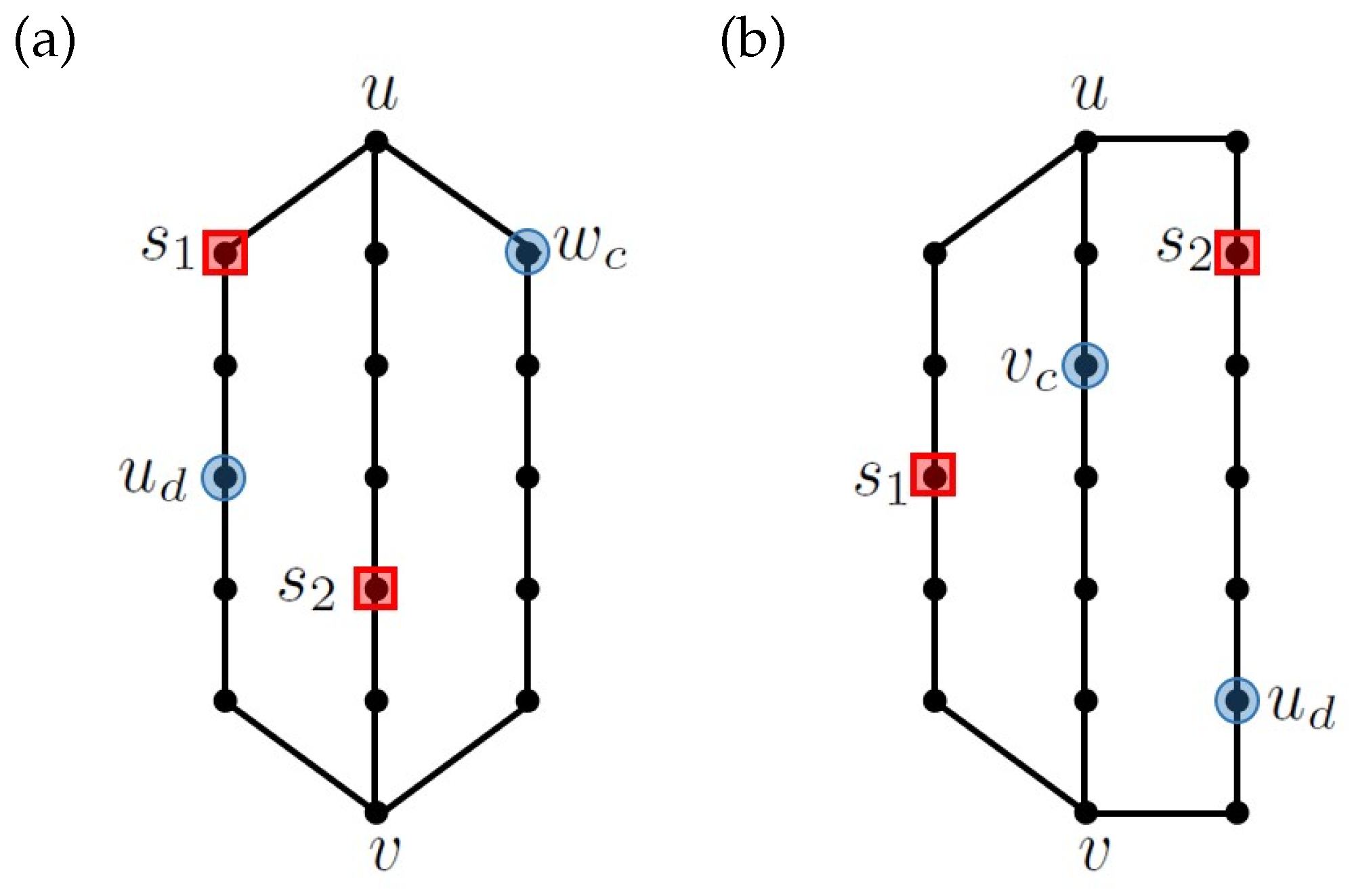
Now, denote by $s_1$ and $s_2$ the two elements of S. Then, $s_1$ and $s_2$ are internal vertices of paths $P_i$ and $P_j$, respectively, where $i\ne j$. We distinguish two cases.

Case 1:$s_1\in V\left(P_1\right)$and$s_2\in V\left(P_2\right)$. Let us denote $d_1=d(s_1,u),$$d_2=d(s_2,u),$ $a=d_1+d_2$, and $b=2p-a$. If $a=b,$ then $s_1$ and $s_2$ form an antipodal pair on $C_{12}$, which implies that two neighbors of $s_1$ are not distinguished by S. Therefore, without loss of generality, we may assume $a<p$ and $d_1\le d_2$. Since $a+b=2p,$ it follows that a and b are of the same parity; hence, $b-a$ is a positive even number. Therefore, we can define $c=(b-a)/2$, and we know that c is a positive integer. Let $d=2d_1+c$. Notice that

$$c<d=2d_1+c\le a+c=\frac{a}{2}+\frac{b}{2}=p.$$

Therefore, there exist interior vertices $u_d\in P_1$ and $w_c\in P_3$; see Figure 1a.

Now, we prove that $u_d$ and $w_c$ are not distinguished by S. Notice that $d(u_d,s_1)=d-d_1=d_1+c.$ Since

$$c+d_1=\frac{b}{2}-\frac{a}{2}+d_1\le \frac{b}{2}=p-\frac{a}{2}<p,$$

we have $d(w_c,s_1)=c+d_1$, and so, $u_d$ and $w_c$ are not distinguished by $s_1$. As for $s_2$, notice that

$$c+d_2<\frac{b-a}{2}+a=p,$$

so we have $d(w_c,s_2)=c+d_2.$ Furthermore, we have

$$d_2+d=d_2+2d_1+c=a+d_1+\frac{b-a}{2}=p+d_1>p,$$

which implies

$$d(u_d,s_2)=2p-d-d_2=2p-p-d_1=p-d_1=p-a+d_2=c+d_2.$$

We conclude that $u_d$ and $w_c$ are not distinguished by $s_2$ either, so S is not a vertex metric generator.

Case 2:$s_1\in V\left(P_1\right)$and$s_2\in V\left(P_3\right)$. For $G={\Theta }_{p,p,p}$, this case is analogous to the previous one, so let us assume $G={\Theta }_{p,p,p+2}$. Again, denote $d_1=d(u,s_1)$, $d_2=d(u,s_2),$$a=d_1+d_2$, and $b=2p+2-a$. If $a=b,$ then $s_1$ and $s_2$ are antipodal on $C_{13}$, so the two neighbors of $s_1$ are not distinguished by S. Hence, without loss of generality, we may assume $a<b.$ Let us denote $c=(b-a)/2.$ Since $a+b=2p+2$ we know that a and b are of the same parity, so $b-a$ is a positive integer. Consequently, also, c is a positive integer.

First, since $s_1$ and $s_2$ are internal vertices of paths $P_1$ and $P_3$, respectively, we have $a=d_1+d_2\ge 2$. This yields

$$c=\frac{b-a}{2}=\frac{a+b}{2}-a=p+1-a\le p-1.$$

Hence, there exists an interior vertex $v_c\in V\left(P_2\right),$ as it is shown in Figure 1b. Furthermore, notice that

$$d_1+c<a+\frac{b-a}{2}=\frac{a+b}{2}=p+1,$$

which implies $d(v_c,s_1)=d_1+c.$

Now, let $d=2d_1+c.$ If $d\le p$, we consider the vertex $u_d\in V\left(P_1\right)$; otherwise, for the sake of simplicity, we denote $u_d=w_{2p+2-d}$; see Figure 1b. We have already shown $d_1+c<p+1$, which yields

$$d-d_1=d_1+c<p+1,$$

and so, $d(u_d,s_1)=d-d_1=d_1+c=d(v_c,s_1)$. Hence, $u_d$ and $v_c$ are not distinguished by $s_1.$ It remains to prove that $u_d$ and $v_c$ are not distinguished by $s_2$ either. For that purpose, notice that

$$c+d_2<c+a=\frac{b-a}{2}+a=\frac{a+b}{2}=p+1,$$

which implies $d(v_c,s_2)=c+d_2.$ Furthermore, notice that

$$\begin{array}{cc}\hfill 2p+2-d-d_2& =a+b-2d_1-c-d_2=a+b-d_1-\frac{b-a}{2}-(d_1+d_2)\hfill \\ \hfill & =\frac{a+b}{2}-d_1=p+1-d_1<p+1,\hfill \end{array}$$

which implies

$$\begin{array}{cc}\hfill d(s_2,u_d)& =2p+2-d-d_2=\frac{a+b}{2}-d_1=\frac{a+b}{2}-a+a-d_1=\hfill \\ \hfill & =\frac{b-a}{2}+d_2=c+d_2=d(v_c,s_2).\hfill \end{array}$$

Therefore, vertices $v_c$ and $u_d$ are not distinguished by $s_2$ either; hence, we conclude that S is not a vertex metric generator. □

Now, a subgraph H of a graph G is an isometric subgraph if $d_H(u,v)=d_G(u,v)$ for every pair of vertices $u,v\in V\left(H\right).$ Consequently, if a pair of vertices is distinguished by $S\cap V\left(H\right)$ in $H,$ then it is distinguished by S in G as well.

Lemma 3.

Let $G={\Theta }_{p,p,p}$ or ${\Theta }_{p,p,p+2}$ with $p\ge 2$. Then. for any $a\in V\left(G\right),$ there are $b,c\in V\left(G\right)$ such that $S=\{a,b,c\}$ is a vertex metric generator in G.

Proof. 

First, notice that every cycle $C_{ij}$ of G is an isometric subgraph in $G.$ We say that a set $S\subseteq V\left(G\right)$ is nice, if for every cycle $C_{ij}$ of G, it holds that $S\cap V\left(C_{ij}\right)$ contains two vertices that do not form an antipodal pair in $C_{ij}$. We first show that any nice set S is a vertex metric generator in $G.$ In order to see this, let x and $x^{\prime }$ be a pair of vertices from $G.$ Notice that x and $x^{\prime }$ belong to at least one cycle $C_{ij}$ in G. Since S is nice, $S\cap V\left(C_{ij}\right)$ contains two vertices that are not antipodal in $C_{ij}$, which implies that $S\cap V\left(C_{ij}\right)$ is a vertex metric generator in $C_{ij}.$ Therefore, x and $x^{\prime }$ are distinguished by $S\cap V\left(C_{ij}\right)$ in $C_{ij}.$ Since $C_{ij}$ is an isometric subgraph of $G,$ this further implies that x and $x^{\prime }$ are distinguished by S in $G,$ so S is a vertex metric generator of G. To complete the proof, for every $a\in V\left(G\right)$, we extend a to a nice set.

Let us assume $G={\Theta }_{p,p,p}.$ If $p\le 3,$ the set $S=\{u,v_1,w_1\}$ is a nice set in G. Therefore, S is a vertex metric generator, which, due to the symmetry of G, proves the claim. Therefore, let us assume that $p\ge 4$. By symmetry, we may assume that $a=u_i$, where $0\le i\le ⌊p/2⌋$. However, then, $S_i=\{u_i,v_1,w_1\}$ is a nice set in G.

Assume now that $G={\Theta }_{p,p,p+2}.$ If $p=2,$ it is easy to see that sets $S=\{u,v_1,w_1\}$ and $S=\{u,v_1,w_2\}$ are nice in $G,$ which, due to the symmetry of G, proves the claim. If $p>2,$ then, due to the symmetry of G, it is sufficient to prove the claim for $a=u_i$, where $0\le i\le ⌊p/2⌋$, and for $a=w_j$, where $1\le j\le ⌊p/2⌋+1.$ If $a=u_i$ for $i\le ⌊p/2⌋,$ then $S=\{u_i,v_1,w_1\}$ is nice in G. On the other hand, if $a=w_j$ for $j\le ⌊p/2⌋+1$, then $S=\{u_1,v_1,w_j\}$ is nice in G. □

By Lemmas 2 and 3, the following statement holds.

Theorem 1.

For $p\ge 2,$ it holds that $\dim \left({\Theta }_{p,p,p}\right)=\dim \left({\Theta }_{p,p,p+2}\right)=3$.

Since, in any $\Theta$-graph G, it holds that $L\left(G\right)=0$ and $c\left(G\right)=2,$ the above theorem gives the following corollary.

Corollary 1.

We have $\dim \left({\Theta }_{p,p,p}\right)=\dim \left({\Theta }_{p,p,p+2}\right)=2c\left(G\right)-1$.

Hence, for ${\Theta }_{p,p,p}$ and ${\Theta }_{p,p,p+2}$, the bound from Conjecture 3 holds with equality. Similarly, when considering the edge metric dimension of $\Theta$-graphs, we have the following.

Lemma 4.

Let $G={\Theta }_{1,2,2}$ or ${\Theta }_{p,p,q}$ with $2\le p\le 3$ and $p\le q\le p+2.$ Then, for any $a\in V\left(G\right),$ there are $b,c\in V\left(G\right)$ such that $S=\{a,b,c\}$ is an edge metric generator in G.

Proof. 

As $p=2$ or 3 and $q\in \{p,p+1,p+2\},$ the problem is finite. To avoid a tedious proof, the statement was easily verified by a computer by checking all sets $S\subseteq V\left(G\right)$ of cardinality three. □

Proposition 1.

Let $G={\Theta }_{1,2,2}$ or ${\Theta }_{p,p,q}$ with $2\le p\le 3$ and $p\le q\le p+2$. Then, $\mathrm{edim}\left(G\right)=3$.

Proof. 

Similarly as before, by a computer, we checked easily that there is no edge metric generator of size two. Then, the claim follows from Lemma 4. □

Corollary 2.

Let $G={\Theta }_{1,2,2}$ or $G={\Theta }_{p,p,q}$ for $2\le p\le 3$ and $p\le q\le p+2$. Then, $\mathrm{edim}\left(G\right)=2c\left(G\right)-1.$

3. $\Theta$-Graphs with Metric Dimensions Equal to 2

In this section, we show that all remaining $\Theta$-graphs, i.e., all $\Theta$-graphs not mentioned in the previous section, have the vertex (respectively the edge) metric dimension equal to 2. We first consider the vertex metric dimension. For all remaining $\Theta$-graphs, we show that there is a set S of cardinality two that is a vertex metric generator; see Figure 2.

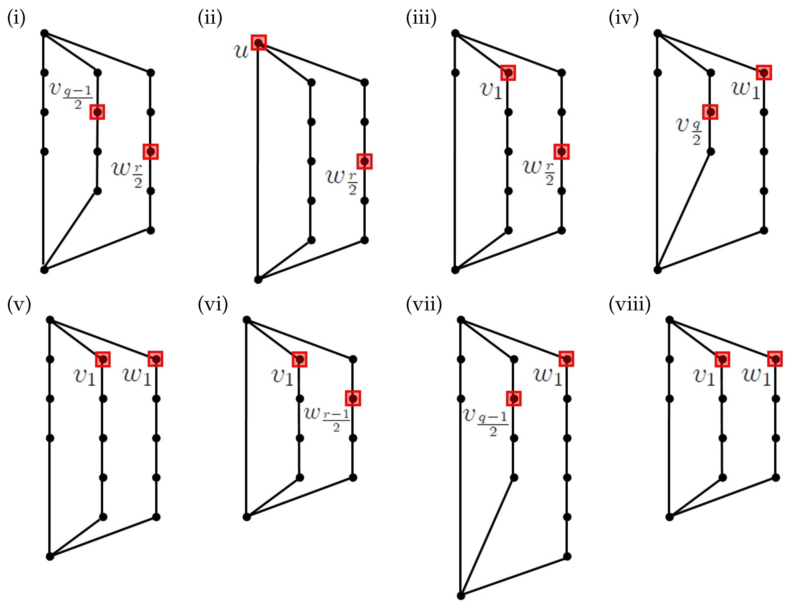
Lemma 5.

Let $G={\Theta }_{p,q,r}$, where $p\le q\le r,$ and let S be a set of vertices in $G,$ defined in the following way:

(i)

If one of p, q, r is odd and at least 3 and one of p, q, r is even, say $q\ge 3$ is odd and r is even, then $S=\{v_{(q-1)/2},w_{r/2}\}$;

(ii)

If $p=1$ and both q and r are even, then $S=\{u,w_{r/2}\}$;

(iii)

If all p, q, r are even and $q\notin \{p,p+2\},$ then $S=\{v_1,w_{r/2}\}$;

(iv)

If all of p, q, r are even, $q\in \{p,p+2\}$, and $r\ge p+4,$ then $S=\{v_{q/2},w_1\}$;

(v)

If all p, q, r are even and $q=r=p+2,$ then $S=\{v_1,w_1\}$;

(vi)

If all p, q, r are odd and $q\notin \{p,p+2\}$, then $S=\{v_1,w_{(r-1)/2}\}$;

(vii)

If all p, q, r are odd, $q\in \{p,p+2\}$ and $r\ge p+4$, then $S=\{v_{(q-1)/2},w_1\}$;

(viii)

If all p, q, r are odd and $q=r=p+2,$ then $S=\{v_1,w_1\}$.

Then, S is a vertex metric generator in $G.$

Proof. 

First, we introduce some notation. For a vertex $a\in V\left(G\right)$, we denote by ${\mathcal{P}}_a$ the partition of $V\left(G\right)$ according to the distances from a. That is, if $x,x^{\prime }$ are in the same set of ${\mathcal{P}}_a$, then $d(a,x)=d(a,x^{\prime })$. To prove that $S=\{a,b\}$ is a vertex metric generator in G, it suffices to show that $d(b,x)\ne d(b,x^{\prime })$ for every pair of vertices $x,x^{\prime }$ from a common set of ${\mathcal{P}}_a$. Proceeding by way of contradiction, if $d(b,x)=d(b,x^{\prime })$, then the shortest path from b to x cannot contain a path from b to $x^{\prime }$ and vice versa. This simplifies our consideration since ${\Theta }_{p,q,r}$ contains only two branching vertices (i.e., vertices of degree at least 3). Let us now consider each of the eight cases separately:

(i) For the vertex $w_{r/2}\in S,$ we have

$${\mathcal{P}}_{w_{\frac{r}{2}}}=(\left\{w_{\frac{r}{2}}\right\},{\{w_i,w_{r-i}\}}_{i=0}^{\frac{r}{2}-1},{\{u_i,v_i,u_{p-i},v_{q-i}\}}_{i=1}^{\lfloor \frac{p}{2}\rfloor },{\{v_i,v_{q-i}\}}_{i=\lfloor \frac{p}{2}\rfloor +1}^{\lfloor \frac{q}{2}\rfloor }).$$

We have to show that the other vertex of $S,$ i.e., $v_{(q-1)/2},$ distinguishes all pairs of vertices from a common set of ${\mathcal{P}}_{w_{\frac{r}{2}}}.$ The first type of set in ${\mathcal{P}}_{w_{\frac{r}{2}}}$ that contains at least one pair of vertices is $\{w_i,w_{r-i}\},$ so we have to show that $w_i$ and $w_{r-i}$ are distinguished by $v_{(q-1)/2},$ and that follows from

$$d(v_{\frac{q-1}{2}},w_i)=i+\frac{q-1}{2}<i+\frac{q+1}{2}=d(w_{\frac{q-1}{2}},w_{r-i}).$$

The next set from ${\mathcal{P}}_{w_{\frac{r}{2}}}$ to consider is of the type $\{u_i,v_i,u_{p-i},v_{q-i}\},$ where we have

$$d(v_{\frac{q-1}{2}},v_i)<d(v_{\frac{q-1}{2}},v_{q-i})<d(v_{\frac{q-1}{2}},u_i)<d(y_{\frac{q-1}{2}},u_{p-i}),$$

where the last two expressions have place only if $i\le \lfloor \frac{p}{2}\rfloor$. Therefore, all pairs of vertices from that set are distinguished by $v_{(q-1)/2}\in S$. Notice that the inequality covers also the last type of set from ${\mathcal{P}}_{w_{\frac{r}{2}}}$. Furthermore, observe that we did not use the fact that $p\le q\le r$ here, so the proof covers all cases when one of $p,q,r$ is odd and at least 3 and one of $p,q,r$ is even.

(ii) Analogously, as in (i), we have

$${\mathcal{P}}_{w_{\frac{r}{2}}}=(\left\{w_{\frac{r}{2}}\right\},{\{w_i,w_{r-i}\}}_{i=0}^{\frac{r}{2}-1},{\{v_i,v_{q-i}\}}_{i=1}^{\frac{q}{2}-1},\left\{v_{\frac{q}{2}}\right\}).$$

It remains to show that u distinguishes all pairs of vertices that belong to a common set of ${\mathcal{P}}_{w_{\frac{r}{2}}}$. This is seen from $d(u,w_i)=i<i+1=d(u,w_{r-i})$ and $d(u,v_i)=i<i+1=d(u,v_{q-i})$.

(iii) We have

$${\mathcal{P}}_{w_{\frac{r}{2}}}=(\left\{w_{\frac{r}{2}}\right\},{\{w_i,w_{r-i}\}}_{i=0}^{\frac{r}{2}-1},{\{u_i,v_i,u_{p-i},v_{q-i}\}}_{i=1}^{\frac{p}{2}},{\{v_i,v_{q-i}\}}_{i=\frac{p}{2}+1}^{\frac{q}{2}}).$$

(Observe that the third set has just three vertices if $i=p/2$, and the last set has just one vertex if $i=q/2$.) We show that $v_1\in S$ distinguishes all pairs of vertices from a common set of ${\mathcal{P}}_{w_{\frac{r}{2}}}$. Regarding set $\{w_i,w_{r-i}\}$, notice that $d(v_1,w_i)=i+1<1+p+i=d(v_1,w_{r-i}).$ The next sets of ${\mathcal{P}}_{w_{\frac{r}{2}}}$ are of the form $\{u_i,v_i,u_{p-i},v_{q-i}\}$, where

$$d(v_1,v_i)=i-1<i+1=d(v_1,u_i),$$

and assuming that $v_1$ does not distinguish the other possible pairs leads to a contradiction, namely $d(v_1,u_i)=d(v_1,u_{p-i})$ implies $i+1=q-1+i$ and $q=2$, a contradiction; $d(v_1,u_i)=d(v_1,v_{q-i})$ implies $i+1=q-i-1$ and $i=q/2-1$, but such $u_i$ exists only if $q\le p+2$, a contradiction; $d(v_1,v_i)=d(v_1,u_{p-i})$ implies $i-1=p-i+1$ and $i=p/2+1$, but such i is over the limit for this set; $d(v_1,v_i)=d(v_1,v_{q-i})$ implies $i-1=1+p+i$ or simplified $p=-2$, a contradiction; $d(v_1,u_{p-i})=d(v_1,v_{q-i})$ implies $1+p-i=q-i-1$ and $q=p+2$, a contradiction.

For the last set of ${\mathcal{P}}_{w_{\frac{r}{2}}}$, we have $d(v_1,v_i)=i-1<q-i-1=d(v_1,v_i)$, whenever $i<q/2$, and for $i=q/2$, the set is a singleton.

(iv) For $v_{q/2}\in S$ we have

$${\mathcal{P}}_{v_{\frac{q}{2}}}=(\left\{v_{\frac{q}{2}}\right\},{\{v_i,v_{q-i}\}}_{i=0}^{\frac{q}{2}-1},{\{u_i,w_i,u_{p-i},w_{r-i}\}}_{i=1}^{\frac{p}{2}},{\{w_i,w_{r-i}\}}_{i=\frac{p}{2}+1}^{\frac{r}{2}}).$$

Now, we consider the distances from $w_1\in S$. Assuming $d(w_1,v_i)=d(w_1,v_{q-i})$ implies $i+1=p+1+i$, so $p=0$, a contradiction.

The next set to consider is of the form $\{u_i,w_i,u_{p-i},w_{r-i}\}$. We have

$$d(w_1,w_i)=i-1<min\{d(w_1,u_i),d(w_1,u_{p-i}),d(w_1,w_{r-i})\},$$

which resolves three of the six possible pairs of vertices. For all other possible pairs, we assume that they are not distinguished by $w_1$ and show that it leads to a contradiction. Namely, $d(w_1,u_i)=d(w_1,u_{p-i})$ implies $i+1=1+q+i$ or simplified $q=0$, a contradiction; $d(w_1,u_i)=d(w_1,w_{r-i})$ implies $i+1=r-i-1$, which reduces to $i=r/2-1$, but such i exceeds the limit for this set, since $r\ge p+4$; $d(w_1,u_{p-i})=d(w_1,w_{r-i})$ implies $1+p-i=r-i-1$, which reduces to $r=p+2$, a contradiction.

For the last set of ${\mathcal{P}}_{v_{\frac{q}{2}}}$, if $w_i\ne w_{r-i}$ and $d(w_1,w_i)=d(w_1,w_{r-i})$, then $i-1=p+1+i$ and $p=-2$, a contradiction.

(v) The partition for $v_1\in S$ is

$${\mathcal{P}}_{v_1}=(\left\{v_1\right\},\{u,v_2\},{\{u_i,v_{i+2},w_i\}}_{i=1}^{p-1},\{v,w_p\},\left\{w_{p+1}\right\}),$$

and for distances from $w_1\in S$, we have

$$\begin{array}{cc}\hfill d(w_1,u)& =1<3=d(w_1,v_2),\hfill \\ \hfill d(w_1,w_i)& =i-1<d(w_1,u_i)=i+1<d(w_1,v_{i+2})=i+3,\hfill \\ \hfill d(w_1,w_p)& =p-1<p+1=d(w_1,v).\hfill \end{array}$$

(vi) For $w_{(r-1)/2}\in S$, we have

$${\mathcal{P}}_{w_{\frac{r-1}{2}}}=(\left\{w_{\frac{r-1}{2}}\right\},{\{w_i,w_{r-i-1}\}}_{i=0}^{\frac{r-3}{2}},\{u_1,v_1,v\},{\{u_i,v_i,u_{p-i+1},v_{q-i+1}\}}_{i=2}^{\frac{p+1}{2}},{\{v_i,v_{q-i+1}\}}_{i=\frac{p+3}{2}}^{\frac{q+1}{2}}).$$

Now, consider the distances from $v_1\in S$. Assume $d(v_1,w_i)=d(v_1,w_{r-i+1})$ implies $i+1=p+1+i+1$, which reduces to $p=-1$, a contradiction.

In the next set $\{u_1,v_1,v\}$ of ${\mathcal{P}}_{w_{\frac{r-1}{2}}}$, there are three possible pairs of vertices, for which we have

$$d(v_1,v_1)=0<d(v_1,u_1)=2<d(v_1,v)=p+1,$$

where the last inequality holds if $p>1$, otherwise $u_1=v$, so there is no pair to be distinguished.

The next set from ${\mathcal{P}}_{w_{\frac{r-1}{2}}}$ is of the type $\{u_i,v_i,u_{p-i+1},v_{q-i+1}\}$, where we first have $d(v_1,v_i)=i-1<i+1=d(v_1,u_i)$, so the pair $u_i,v_i$ is distinguished by $v_1\in S$. For all remaining pairs of vertices from that set, we show that assuming they are not distinguished by $s_1\in S$ leads to a contradiction. If $d(v_1,u_i)=d(v_1,u_{p-i+1})$, then $i+1=q-1+i-1$ and $q=3$, a contradiction; if $d(v_1,u_i)=d(v_1,v_{q-i+1})$, then $i+1=q-i+1-1$, which reduces to $i=(q-1)/2$, but such i exceeds the limit since $q>p+2$; if $d(v_1,v_i)=d(v_1,u_{p-i+1})$, then $i-1=1+p-i+1$ and, therefore, $i=(p+3)/2$, but such i exceeds the limit; if $d(v_1,v_i)=d(v_1,v_{q-i+1})$, then $i-1=1+p+i-1$, which reduces to $p=-1$, a contradiction; finally, if $d(v_1,u_{p-i+1})=d(v_1,v_{q-i+1})$, then $1+p-i+1=q-i+1-1$, and therefore, $q=p+2$, a contradiction.

As for the last type of set in ${\mathcal{P}}_{w_{\frac{r-1}{2}}}$, if $v_i\ne v_{q-i+1}$ and $d(v_1,v_i)=d(v_1,v_{q-i+1})$, then $i-1=1+p+i-1$, and so, $p=-1$, a contradiction.

(vii) Observe that

$${\mathcal{P}}_{v_{\frac{q-1}{2}}}=(\left\{v_{\frac{q-1}{2}}\right\},{\{v_i,v_{q-i-1}\}}_{i=0}^{\frac{q-3}{2}},\{u_1,w_1,v\},{\{u_i,w_i,u_{p-i+1},w_{r-i+1}\}}_{i=2}^{\frac{p+1}{2}},{\{w_i,w_{r-i+1}\}}_{i=\frac{p+3}{2}}^{\frac{r+1}{2}}).$$

Now, we consider the distances from $w_1\in S$. If $d(w_1,v_i)=d(w_1,v_{q-i-1})$, then $i+1=p+1+i+1$ and $p=-1$, a contradiction.

As for the set $\{u_1,w_1,v\}\in {\mathcal{P}}_{v_{\frac{q-1}{2}}},$ we have

$$d(w_1,w_1)=0<d(w_1,u_1)=2<d(w_1,v)=r-1.$$

Therefore, all three pairs of vertices from this set are distinguished by $w_1$.

For the next set of ${\mathcal{P}}_{v_{\frac{q-1}{2}}}$, we first have

$$d(w_1,w_i)=i-1<min\{d(w_1,u_i),d(w_1,u_{p-i+1}),d(w_1,w_{r-i+1})\},$$

so $w_1$ distinguishes $w_i$ from all the other vertices in that set. If $d(w_1,u_i)=d(w_1,u_{p-i+1})$, then $i+1=1+q+i-1$ and $q=1$, a contradiction. If $d(w_1,u_i)=d(w_1,w_{r-i+1})$, then $i+1=r-i+1-1$ and $i=(r-1)/2\ge (p+3)/2$, but such i exceeds the limit. Finally, $d(w_1,u_{p-i+1})=d(w_1,w_{r-i+1})$ implies $1+p-i+1=r-i+1-1$, which reduces to $r=p+2$, a contradiction.

For the last set of ${\mathcal{P}}_{v_{\frac{q-1}{2}}}$, if $w_i\ne w_{r-i+1}$ and $d(w_1,w_i)=d(w_1,w_{r-i+1})$, then $i-1=1+p+i-1$ and $p=-1$, a contradiction.

(viii) Observe that

$${\mathcal{P}}_{v_1}=(\left\{v_1\right\},\{u,v_2\},{\{u_i,v_{i+2},w_i\}}_{i=1}^{p-1},\{v,w_p\},\left\{w_{p+1}\right\}).$$

Hence, ${\mathcal{P}}_{v_1}$ (and also, ${\mathcal{P}}_{w_1}$) does not depend on the parity of p. Therefore, analogous to case (v), one can show that $S=\{v_1,w_1\}$ is a vertex metric generator in this case. □

Using Lemma 5, we can prove that all $\Theta$-graphs not mentioned in the previous section have metric dimension 2.

Theorem 2.

Let G be a Θ-graph such that $G\ne {\Theta }_{p,p,p}$ and ${\Theta }_{p,p,p+2}$ with $p\ge 2.$ Then, $\dim \left(G\right)=2.$

Proof. 

It is sufficient to show that Lemma 5 includes all $\Theta$-graphs distinct from ${\Theta }_{p,p,p}$ and ${\Theta }_{p,p,p+2}$. Cases (iii)-(v) of this lemma obviously include all $\Theta$-graphs distinct from ${\Theta }_{p,p,p}$ and ${\Theta }_{p,p,p+2}$ in which all three parameters p, q, and r are even. Similarly, cases (vi)–(viii) of the same lemma include all $\Theta$-graphs in which all three parameters are odd. It remains to show that cases (i)–(ii) cover all $\Theta$-graphs in which p, q, and r do not have the same parity. In that case, at least one of the parameters is odd. If none of the parameters is equal to one, then Lemma 5. (i) covers the cases. If there is parameter equal to 1, then $p=1$, since $p\le q\le r$. Since G has no parallel edges, $q\ge 2$. Hence, if one of q and r is odd, then this parameter is at least 3 and the other parameter is even, which is covered by Lemma 5. (i) again. The only remaining case when $p=1$ and both q and r are even is covered by Lemma 5. (ii). □

As regards the motivating question for this investigation, Theorem 2 yields the following corollary.

Corollary 3.

Let G be a Θ-graph such that $G\ne {\Theta }_{p,p,p}$ and $G\ne {\Theta }_{p,p,p+2}$. Then, $\dim \left(G\right)<2c\left(G\right)-1$.

Now, we consider the edge metric dimension of $\Theta$-graphs. We proceed analogously as in the case of vertex metric dimension. The edge metric generators from the following lemma are illustrated in Figure 3.

Lemma 6.

Let $G={\Theta }_{p,q,r},$ where $p\le q\le r$, and let S be a set of vertices in G defined in the following way:

(i)

If $p<q$, $r\ge 3$, and $p+r$ is even, then $S=\{w_{(r-p)/2},w_{(r+p)/2}\}$;

(ii)

If $p<q$, $r\ge p+3$, and $p+r$ is odd, then $S=\{w_{\lfloor (r-p)/2\rfloor },w_{\lceil (r+p)/2\rceil }\}$;

(iii)

If $p<q$, $r=p+1$, and $(p,q,r)\ne (1,2,2)$, then $S=\{v_1,w_1\}$;

(iv)

If $p=q$ and $p\ge 4$, then $S=\{u_2,v_1\}$;

(v)

If $p=q$ and $r\ge p+3$, then $S=\{v_1,w_1\}$.

Then, S is an edge metric generator in G.

Proof. 

The proof is analogous to the proof of Lemma 5. Let a be a vertex in G. By ${\mathcal{P}}_a^e$, we denote the partition of $E\left(G\right)$ according to the distances from a. To prove that $S=\{a,b\}$ is an edge metric generator for G, it suffices to show that $d(b,e)\ne d(b,f)$ for every pair of edges $e,f$ from a common set of ${\mathcal{P}}_a^e$. Furthermore, to abbreviate the notation, an edge $u_i{u}_{i+1}$ will be denoted by $u_i^{+}$ or $u_{i+1}^{-},$ and a similar notation will be used for edges $v_i{v}_{i+1}$ and $w_i{w}_{i+1}$. We now consider each of the five cases separately:

(i) Denote $a=(r-p)/2$ and $b=(r+p)/2$. Then, for $w_a\in S$, we have

$${\mathcal{P}}_{w_a}^e=({\{w_{a-i}^{-},w_{a+i}^{+}\}}_{i=0}^{a-1},{\{u_i^{+},v_i^{+},w_{r-p+i}^{+}\}}_{i=0}^{p-1},{\{v_{p+i}^{+},v_{q-i}^{-}\}}_{i=0}^{\lfloor \frac{q-p}{2}\rfloor }).$$

Next, we suppose that $w_b$ has the same distance to a pair of edges from a common set of ${\mathcal{P}}_{w_a}^e$, and we always come to a contradiction. Here, and in the next cases, the first distance is denoted by $d_1$ and the second distance is denoted by $d_2$.

Let us first consider the set $\{w_{a-i}^{-},w_{a+i}^{+}\}$ from ${\mathcal{P}}_{w_a}^e.$ If $d(w_b,w_{a-i}^{-})=d(w_b,w_{a+i}^{+})$, then $d_1=d(w_b,w_{a-i})$. Further, $d_2=d(w_b,w_{a+i})$ (otherwise, $d_2<d_1$), and so, $d(w_b,w_{a-i})=d(w_b,w_{a+i})$. Consequently, $b-(a-i)=(a+i)-b$, and therefore, $a=b$, which contradicts $p\ge 1$.

Let us now consider the set $\{u_i^{+},v_i^{+},w_{r-p+i}^{+}\}\in {\mathcal{P}}_{w_a}^e$ and the distances from $w_b$ to the three possible pairs of edges from this set. If $d(w_b,u_i^{+})=d(w_b,v_i^{+})$, then $d_1=d(w_b,u_{i+1})$, since $d_1<d(w_a,v)=d(w_b,u)$. Analogously, $d_2=d(w_b,v_{i+1})$. Thus, $p-(i+1)=q-(i+1)$ and $p=q$, a contradiction. The next pair is $u_i^{+}$ and $w_{r-p+i}^{+},$ where assuming $d(w_b,u_i^{+})=d(w_b,w_{r-p+i}^{+})$ yields $d_1=d(w_b,u_{i+1})$ and $d_2=d(w_b,w_{r-p+i+1})$. Thus,

$$r-\frac{r+p}{2}+p-(i+1)=\frac{r+p}{2}-(r-p+i+1)$$

which reduces to $r=p$, a contradiction. The last pair is $v_i^{+}$ and $w_{r-p+i}^{+},$ in which case $d(w_b,v_i^{+})=d(w_b,w_{r-p+i}^{+})$ implies $d_2>d(w_b,v)=d(w_a,u)$, and so, $d_2=d(w_b,w_{r-p+i+1})$ and $d_1=d(w_b,v_{i+1})$. This gives

$$r-\frac{r+p}{2}+q-(i+1)=\frac{r+p}{2}-(r-p+i+1)$$

and $r+q=2p$, a contradiction.

It remains to consider the set $\{v_{p+i}^{+},v_{q-i}^{-}\}\in {\mathcal{P}}_{w_a}^e$. Assuming $d(w_b,v_{p+i}^{+})=d(w_b,v_{q-i}^{-})$ yields $d_2=d(w_b,v_{q-i})=d(w_b,v)+d(v,v_{q-i})$. However, $d(\{u,v\},\{v_{p+i},v_{p+i+1}\})>d(v,v_{q-i})$ and $d(\{u,v\},w_b)\ge d(w_b,v)$. Therefore, $d_1>d_2$, a contradiction.

(ii) Since $r\ge p+3$, we have $\lfloor (r-p)/2\rfloor \ge \lfloor 3/2\rfloor =1$. Since $p\ge 1$, we have $\lfloor (r-p)/2\rfloor <\lceil (r+p)/2\rceil$. Hence, $1\le \lfloor (r-p)/2\rfloor <\lfloor r/2\rfloor$. Denote $a=\lfloor (r-p)/2\rfloor$ and $b=\lceil (r+p)/2\rceil$. Then, for $w_a\in S$, we have

$${\mathcal{P}}_{w_a}^e=({\{w_{a-i}^{-},w_{a+i}^{+}\}}_{i=0}^{a-1},{\{u_i^{+},v_i^{+},w_{2a+i}^{+}\}}_{i=0}^{p-1},\{v_p^{+},v_q^{-},w_{r-1}^{+}\},{\{v_{p+i}^{+},v_{q-i}^{-}\}}_{i=1}^{\lfloor \frac{q-p-1}{2}\rfloor }).$$

For each of the sets from ${\mathcal{P}}_{w_a}^e$, we now show that all possible pairs of edges from that set are distinguished by $w_b\in S$. Let us first consider the set $\{w_{a-i}^{-},w_{a+i}^{+}\}$. Assuming $d(w_b,w_{a-i}^{-})=d(w_b,w_{a+i}^{+})$, analogous as in (i), we obtain $a=b$, which contradicts $p\ge 1$.

Now, consider $\{u_i^{+},v_i^{+},w_{2a+i}^{+}\}$. If $d(w_b,u_i^{+})=d(w_b,v_i^{+})$, then analogously as in (i), we obtain $p=q$, a contradiction. If $d(w_b,u_i^{+})=d(w_b,w_{2a+i}^{+})$, then $d_1=d(w_b,u_{i+1})$ and $d_2=d(w_b,w_{2a+i+1})$. Thus,

$$r-\frac{r+p+1}{2}+p-(i+1)=\frac{r+p+1}{2}-(2\frac{r-p-1}{2}+i+1)$$

which reduces to $r=p+2$, a contradiction. Finally, if $d(w_b,v_i^{+})=d(w_b,w_{2a+i}^{+})$, then $d_1=d(w_b,v_{i+1})$ and $d_2=d(w_b,w_{2a+i+1})$. Thus,

$$r-\frac{r+p+1}{2}+q-(i+1)=\frac{r+p+1}{2}-(2\frac{r-p-1}{2}+i+1)$$

and hence, $r+q=2p+2$, a contradiction.

For edges from $\{v_p^{+},v_q^{-},w_{r-1}^{+}\}$, we have $d(w_b,w_{r-1}^{+})=d(w_b,w_{r-1})=r-b-1$ and $d(w_b,v_q^{-})=d(w_b,v)=r-b$, so that $d(w_b,w_{r-1}^{+})<d(w_b,v_q^{-})$. If $d(w_b,w_{r-1}^{+})=d(w_b,v_p^{+})$, then $d_2=d(w_b,v_p)$. Therefore, $r-b-1=b+p$, and consequently, $r-p-1=2b=r+p+1$, a contradiction. Finally, if $d(w_b,v_q^{-})=d(w_b,v_p^{+})$, then $d_2=d(w_b,v_p)$. Therefore, $r-b=b+p$, and consequently, $r-p=2b=r+p+1$, a contradiction.

Finally, consider $\{v_{p+i}^{+},v_{q-i}^{-}\}$. Assuming $d(w_b,v_{p+i}^{+})=d(w_b,v_{q-i}^{-})$ yields

$$\begin{array}{cc}\hfill d_2& =d(w_b,v_{q-i})=d(w_b,v)+d(v,v_{q-i})\hfill \\ \hfill & <min\{d(\{u,v\},\{v_{p+i},v_{p+i+1}\})+d(w_b,\{u,v\})\}\le d_1,\hfill \end{array}$$

a contradiction.

(iii) Notice that, in this case, $G={\Theta }_{p,p+1,p+1}$, where $p\ge 2$. For $v_1\in S$, the partition is

$${\mathcal{P}}_{v_1}^e=(\{v_1^{-},v_1^{+}\},{\{u_i^{+},v_{i+2}^{+},w_i^{+}\}}_{i=0}^{p-2},\{u_{p-1}^{+},w_{p-1}^{+},w_{p+1}^{-}\}).$$

First, consider the set $\{v_1^{-},v_1^{+}\}$. Since $p\ge 2$, we have $d(w_1,v_1^{-})=1<2=d(w_1,v_1^{+})$, so $v_1^{-}$ and $v_1^{+}$ are distinguished by $w_1\in S$.

Now, consider $\{u_i^{+},v_{i+2}^{+},w_i^{+}\}$. Since

$$d(w_1,w_i^{+})\le i<d(w_1,u_i^{+})=i+1<i+2\le d(w_1,v_{i+2}^{+}),$$

all three pairs are distinguished by $w_1\in S.$

Finally, for $\{u_{p-1}^{+},w_{p-1}^{+},w_{p+1}^{-}\}$, we have

$$d(w_1,w_{p-1}^{+})=p-2<d(w_1,w_{p+1}^{-})=p-1<d(w_1,u_{p-1}^{+})=p.$$

(iv) Observe that

$${\mathcal{P}}_{v_1}^e=(\{v_1^{-},v_1^{+}\},{\{u_i^{+},v_{i+2}^{+},w_i^{+}\}}_{i=0}^{p-3},\{u_{p-2}^{+},u_p^{-},w_{p-2}^{+},w_r^{-}\},{\{w_{p-1+i}^{+},w_{r-1-i}^{-}\}}_{i=0}^{\lceil \frac{r-p}{2}\rceil }).$$

First, for the unique pair from $\{v_1^{-},v_1^{+}\}$, it holds that $d(u_2,v_1^{-})=2<d(u_2,v_1^{+})=3$ if $p\ge 4$, so it is distinguished by $u_2$.

Next, consider $\{u_i^{+},v_{i+2}^{+},w_i^{+}\}$. Suppose that $d(u_2,u_i^{+})=d(u_2,v_{i+2}^{+})$. If $i\ge 2$, then $d_1=i-2$, and consequently, $d_2=i+4$, a contradiction. Hence, $0\le i\le 2$ and

$$d(u_2,u_i^{+})=d(u_2,u_{i+1})=1-i<d(u_2,v_{i+2}^{+})=d(u_2,v_{i+3})=p-2+p-(i+3),$$

a contradiction. For the second pair $u_i^{+}$ and $w_i^{+}$, since $i\le p-3$, we have

$$d(u_2,u_i^{+})\le (i-2)+3<i+2=d(u_2,w_i)=d(u_2,w_i^{+}).$$

For the last pair $v_{i+2}^{+}$ and $w_i^{+},$ we assume that $d(u_2,v_{i+2}^{+})=d(u_2,w_i^{+})$. We distinguish three subcases:

-

If $0\le i\le p-5$, then $d_1=d(u_2,v_{i+2})=i+4>i+2=d(u_2,w_i)=d_2$;

-

If $i=p-4$, then $d_1=d(u_2,v_{i+3})=p-1>p-2=d(u_2,w_i)=d_2$;

-

If $i=p-3$, then $d_1=d(u_2,v_{i+3})=p-2<p-1=d(u_2,w_i)=d_2$.

Now, we consider the set $\{u_{p-2}^{+},u_p^{-},w_{p-2}^{+},w_r^{-}\}$. We have

$$d(u_2,u_{p-2}^{+})=p-4<d(u_2,u_p^{-})=p-3<d(u_2,w_r^{-})=p-2<d(u_2,w_{p-2}^{+})\ge p-1,$$

where the last inequality is an equality only if $r=p$.

Finally, for $\{w_{p-1+i}^{+},w_{r-1-i}^{-}\}$, suppose that $d(u_2,w_{p-1+i}^{+})=d(u_2,w_{r-1-i}^{-})$. Then, $d_2=d(u_2,w_{r-1-i})$, and so, $d_1=d(u_2,w_{p-1+i})$. Thus, $2+p-1+i=p-2+r-(r-1-i)$ and $1=-1$, a contradiction.

(v) Observe that

$${\mathcal{P}}_{v_1}^e=(\{v_1^{-},v_1^{+}\},{\{u_i^{+},v_{i+2}^{+},w_i^{+}\}}_{i=0}^{p-3},\{u_{p-2}^{+},u_p^{-},w_{p-2}^{+},w_r^{-}\},{\{w_{p-1+i}^{+},w_{r-1-i}^{-}\}}_{i=0}^{\lceil \frac{r-p}{2}\rceil }).$$

First, consider the set $\{v_1^{-},v_1^{+}\}$. Since $r\ge 4$, we have $d(w_1,v_1^{-})=1<2=d(w_1,v_1^{+})$.

Next, consider the set $\{u_i^{+},v_{i+2}^{+},w_i^{+}\}$. We have

$$d(w_1,v_{i+2}^{+})=i+3>d(w_1,u_i^{+})=i+1>d(w_1,w_i^{+})\le i,$$

where the last inequality is an equality only if $i=0$ and the first equality is a consequence of $r\ge p+3$.

Now, consider the set $\{u_{p-2}^{+},u_p^{-},w_{p-2}^{+},w_r^{-}\}$. We have

$$d(w_1,w_{p-2}^{+})=p-3<d(w_1,u_{p-2}^{+})=p-1<d(w_1,u_p^{-})=p<d(w_1,w_r^{-})=p+1,$$

where the last inequality holds since $r\ge p+3$.

Finally, consider the set $\{w_{p-1+i}^{+},w_{r-1-i}^{-}\}$. If $d(w_1,w_{p-1+i}^{+})=d(w_1,w_{r-1-i}^{-})$, then $d_1=d(w_1,w_{p-1+i})$, and so, $d_2=d(w_1,w_{r-1-i})$. Thus, $p-1+i-1=1+p+r-(r-1-i)$ and $-2=2$, a contradiction. This concludes the proof. □

The following statement is a consequence of Lemma 6.

Theorem 3.

Let G be a Θ-graph such that $G\ne {\Theta }_{1,2,2}$ and ${\Theta }_{p,p,q}$ for $2\le p\le 3$ and $p\le q\le p+2$. Then, $\mathrm{edim}\left(G\right)=2$.

Proof. 

First suppose that $p<q$. If $p+r$ is even, then $r\ge 3$, so Lemma 6. (i) covers this case. On the other hand, if $p+r$ is odd, then $r\ge p+1$, so Lemma 6. (ii) and Lemma 6. (iii) cover all cases except ${\Theta }_{1,2,2}$.

Now, suppose that $p=q$. Then, Lemma 6. (v) covers all cases, except ${\Theta }_{p,p,p}$, ${\Theta }_{p,p,p+1}$, and ${\Theta }_{p,p,p+2}$. These remaining cases are covered by Lemma 6. (iv) when $p\ge 4$. Hence, uncovered cases are ${\Theta }_{2,2,2}$, ${\Theta }_{2,2,3}$, ${\Theta }_{2,2,4}$, ${\Theta }_{3,3,3}$, ${\Theta }_{3,3,4}$, and ${\Theta }_{3,3,5}$. □

Supporting our motivation, Theorem 3 yields the following corollary.

Corollary 4.

Let G be a Θ-graph such that $G\ne {\Theta }_{1,2,2}$ and ${\Theta }_{p,p,q}$ for $2\le p\le 3$ and $p\le q\le p+2$. Then, $\mathrm{edim}\left(G\right)<2c\left(G\right)-1.$

4. Further Work

In this paper, we investigated Conjecture 3 (respectively Conjecture 4), which states that the vertex (respectively the edge) metric dimension of a graph $G\ne C_n$ with $\delta \left(G\right)\ge 2$ is bounded above by $2c\left(G\right)-1$. It was established in [26] that the conjectures hold for cacti without leaves and that, for other leafless graphs, the problem reduces to 2-connected graphs, i.e., if the conjectures hold for 2-connected graphs distinct from a cycle, then they hold in general. In this paper, we considered $\Theta$-graphs, since they are the most simple 2-connected graphs distinct from cycles. We established that Conjectures 3 and 4 hold on this class of graphs, and we characterized all $\Theta$-graphs for which the upper bound is attained.

Besides $\Theta$-graphs attaining the upper bound $2c\left(G\right)-1$, it was previously established that the same upper bound is also attained by metric dimensions of some leafless cacti. To be more precise, a daisy graph is any graph consisting of at least two cycles that all share the same vertex. A cycle in a daisy graph is also called a petal. Now, it was established that $\dim \left(G\right)$ attains the bound $2c\left(G\right)-1$ if G is a daisy graph without odd petals and that $\mathrm{edim}\left(G\right)$ reaches the same bound for any daisy graph G. We expect that these graphs are the only graphs with $\delta \left(G\right)\ge 2$ whose metric dimensions reach the bound. Therefore, we conclude the paper by stating the following two conjectures.

Conjecture 5.

Let G be a connected graph with $\delta \left(G\right)\ge 2$. Then, $\dim \left(G\right)=2c\left(G\right)-1$ if and only if G is a daisy graph without odd petals, $G={\Theta }_{p,p,p}$ or $G={\Theta }_{p,p,p+2}.$

Conjecture 6.

Let G be a connected graph with $\delta \left(G\right)\ge 2$. Then, $\mathrm{edim}\left(G\right)=2c\left(G\right)-1$ if and only if G is a daisy graph, $G={\Theta }_{1,2,2}$ or $G={\Theta }_{p,p,q}$ with $2\le p\le 3$ and $p\le q\le p+2.$

Similar as with Conjectures 3 and 4, we show in the next proposition that the above two conjectures reduce to the same problem on 2-connected graphs. In order to do so, we use a result from [26], which states that $c\left(G\right)=c\left(G_1\right)+\cdots +c\left(G_q\right)$ where $G_1,\dots ,G_q$ is the complete list of blocks of G.

Proposition 2.

If Conjecture 5 (respectively Conjecture 6) holds for 2-connected graphs, then it holds in general.

Proof. 

We say that G is vertex extremal, if $G={\Theta }_{p,p,p}$ or $G={\Theta }_{p,p,p+2}.$ We say G is edge extremal if $G={\Theta }_{1,2,2}$ or $G={\Theta }_{p,p,q}$ for $2\le p\le 3$ and $p\le q\le p+2.$ Now, let G be a graph with $\delta \left(G\right)\ge 2$, which is not 2-connected. According to Lemma 1, the equality $\dim \left(G\right)=2c\left(G\right)-1$ (respectively $\mathrm{edim}\left(G\right)=2c\left(G\right)-1$) may hold only when every non-trivial block of G distinct from a cycle is vertex extremal (respectively edge extremal) and all blocks of G share a vertex.

We shall now construct a vertex (respectively an edge) metric generator in such a graph whose size is smaller than $2c\left(G\right)-1,$ which is sufficient to prove the claim. Let v be a vertex of G shared by all blocks in $G.$ Let us assume $G_1,\dots ,G_q$ are all non-trivial blocks in G denoted so that $G_i$ is a cycle whenever $i>p.$ According to Lemma 3 (respectively Lemma 4), for $1\le i\le p$, there is a vertex (respectively an edge) metric generator $S_i^{\prime }$ in $G_i$ such that $v\in S_i^{\prime },$ and for such i, let us denote $S_i=S_i^{\prime }\backslash \left\{v\right\}$. For $i>p,$ let $S_i$ consist of a single vertex, which is a neighbor of v in $G_i.$ Now, let $S=S_1\cup \cdots \cup S_q.$ Observe that the set S distinguishes in G all pairs of vertices (respectively edges) that belong to the same block of G; this follows from the fact that a pair of vertices (respectively edges) that is distinguished by v in $G_i$ is in G distinguished by every vertex $s\in S\backslash V\left(G_i\right).$

By the above, a pair of vertices (respectively edges) x and $x^{\prime }$ is not distinguished by S in G only if x belongs to $G_i$ and $x^{\prime }$ belongs to $G_j$, $i\ne j$. In such a case, we say $G_i$ and $G_j$ are critically incident. Therefore, let $G_i$ and $G_j$ be critically incident with $x\in V\left(G_i\right)$, $x^{\prime }\in V\left(G_j\right)$ such that x and $x^{\prime }$ are not distinguished by S. Let further $s\in S_i$ and $s^{\prime }\in S_j$. Then, $d(s,x)=d(s,x^{\prime })$ and $d(s^{\prime },x)=d(s^{\prime },x^{\prime })$. Denote $a=d(s,v)$, $b=d(v,x)$, $c=d(s^{\prime },v)$ and $d=d(v,x^{\prime })$. Then,

$$\begin{array}{cc}\hfill (a+d)+(c+b)& =d(s,x^{\prime })+d(s^{\prime },x)=d(s,x)+d(s^{\prime },x^{\prime })\hfill \\ \hfill & \le d(s,v)+d(v,x)+d(s^{\prime },v)+d(v,x^{\prime })=a+b+c+d,\hfill \end{array}$$

and so, a shortest path from x (respectively $x^{\prime }$) to every vertex from $S_i$ (respectively $S_j$) leads through v. Hence, $b=d$ and $a=c$.

If $b>1$, then let $x_1$ (respectively $x_1^{\prime }$) be a neighbor of x (respectively $x^{\prime }$) on a shortest path from v to x (respectively $x^{\prime }$). Then, for every $s^{\ast }\in S_i\cup S_j$, we have $d(s^{\ast },x_1)=d(s^{\ast },x_1^{\prime })=a+b-1$, so $x_1$ and $x_1^{\prime }$ are not distinguished by S as well.

Finally, let $x_2$ and $x_2^{\prime }$ be another pair of vertices that is not distinguished by S, $x_2\in V\left(G_i\right)$, and $x_2^{\prime }\in V\left(G_j\right)$, and let $d(v,x_2)=d(v,x)$. Then, x and $x_2$ are not distinguished by $S_i$, which means that $x_2=x$ and, analogously, $x_2^{\prime }=x^{\prime }$.

Thus, vertices $y\in V\left(G_i\right)$, for which there exists $y^{\prime }\in V\left(G_j\right)$ such that $y,y^{\prime }$ is a pair not distinguished by S, form a path starting at a neighbor of v. Denote this neighbor by z. If there is $k\ne j$ such that $G_i$ and $G_k$ are critically incident as well, then, again, vertices $y\in V\left(G_i\right)$, for which there exists $y^{\ast }\in V\left(G_k\right)$ such that $y,y^{\ast }$ is a pair not distinguished by S, form a path starting at z. Therefore, it is sufficient to add z to $S_i$, and all pairs of vertices from $G_i$ and $G_k$ (as well as from $G_i$ and $G_j$) will be distinguished.

We conclude that it is sufficient to introduce to S at most $q-1$ vertices, and all pairs x and $x^{\prime }$ from distinct blocks will also be distinguished by $S.$ Consequently, since $\left|S_i\right|=\dim \left(G_i\right)-1$, we have

$$\begin{array}{cc}\hfill \dim \left(G\right)& \le \sum _{i=1}^q(\dim \left(G_i\right)-1)+q-1=\sum _{i=1}^q\dim \left(G_i\right)-1\hfill \\ \hfill & =\sum _{i=1}^p(2c\left(G_i\right)-1)+\sum _{i=p+1}^{q}2c\left(G_i\right)-1=2c\left(G\right)-p-1\hfill \end{array}$$

which is obviously smaller than $2c\left(G\right)-1$ for $p\ge 1.$ If $p=0,$ then G is a cactus graph, and for cacti, it was already established that the bound is attained only for daisy graphs without odd petals. The proof for $\mathrm{edim}\left(G\right)$ is analogous. □