The Allocation of Base Stations with Region Clustering and Single-Objective Nonlinear Optimization

Abstract

For the problem of 5G network planning, a certain number of locations should be selected to build new base stations in order to solve the weak coverage problems of the existing network. Considering the construction cost and some other factors, it is impossible to cover all the weak coverage areas so it is necessary to consider the business volume and give priority to build new stations in the weak coverage areas with high business volume. Aimed at these problems, the clustering of weak point data was carried out by using k-means clustering algorithm. With the objective function as the minimization of the total construction cost of the new base stations, as well as the constraints as the minimal distance between adjacent base stations and the minimal coverage of the communication traffic, the single-objective nonlinear programming models were established to obtain the layout of macro and micro base stations in order to illustrate the impact of the shape of the station coverage area, the circular and the “shamrock” shaped coverage areas were compared in this paper. For the “shamrock” base station, a secondary clustering was undertaken to judge the main directions of the three sector coverage areas. Then, an improved model taking the coverage overlapping into consideration was proposed to correct the coverage area of different sectors. Finally, the optimal layout was obtained by adjusting the distribution of all base stations globally. The results show that the optimal planning method proposed in this paper has good practicability, which also provides a very good reference for solving similar allocation problems of dynamic resources.

1. Introduction

The location–allocation problem is a classic mathematical optimization problem that determines the best location for a facility to be placed based on geographical demands, facility costs, and transportation distances. They are widely utilized in many industries to find the optimal placement of various facilities, including public transportation terminals, power plants, polling locations, warehouses, and cell towers, to maximize efficiency, impact, and profit [1].

With the rapid development of mobile communication technology, its operation scale is getting bigger and bigger; the communication network is getting more and more complex. Especially with the arrival of the 5G era, the effective range that a base station can cover is getting smaller and smaller with the increase of the communication bandwidth. At the same time, with the increasing types of base stations and antennas, communication network planning—especially the site selection of base stations—is more complex.

Generally, base station planning is usually considered as a typical single-objective or multi-objective programming problem. The location and the configuration of base stations have to be chosen so that the majority of the traffic is served, while at the same time the amount of interference and multi-coverage is kept minimal [2]. During this process, the selection of the best location is only a decision variable. The ultimate goal of the selection is usually to achieve the shortest weighted distance, to minimize the cost of network construction, to maximize energy efficiency, or to obtain the optimal site layout scheme, while considering the optimal signal coverage.

For a given area requiring base station planning, a large number of weak signal coverage points scatter in this region. The attributes of each weak coverage point include the location coordinates and the mobile data traffic (the data volume transmitted over mobile networks). In practical network planning, it is almost impossible to cover all weak coverage points due to the prohibitive construction cost and the geographical constrains. Therefore, it is necessary to consider the volume of business and to give priority to the area with high traffic volume. Conventionally, when 90% of the total traffic volume in the area was covered, the construction scheme was considered to have met the deployment requirements [3]. Besides, the shape of the signal coverage domain is very important for planning the base station, but it is in general assumed to be a circle, and there are few discussions on planning the base station combining signal coverage in a “shamrock” shape.

The objective of this work is to build the optimization model of planning base stations in consideration of the actual shape of the coverage area. The main contributions of this paper are the following: (1) the clustering of weak point data was implemented by the k-means clustering; (2) two different single-objective nonlinear programming models were established to obtain the layout scheme of base stations; and (3) discussion and comparison of two cases with a circular coverage area and “shamrock” shaped areas.

The rest of this paper is organized as follows: Section 2 presents the previous work on base station selection. Section 3 introduces the preprocess of the original data. Section 4 shows the establishment of the single-objective nonlinear programming models. Section 5 discusses the obtained results. Section 6 concludes the entire work and gives an outlook for future work.

2. Related Works

In this section, we focus on related works about the optimization location–allocation problem of macro and micro base stations.

A variety of according analytical optimization problems were introduced by Mathar et al. [2] in 2000. Each was formalized as an integer linear program, and the optimum solutions can be given in most cases. When the exact solution cannot be obtained due to the complexity of the problem, simulated annealing was used as an approximate optimization technique. Besides, in 2001, Mathar et al. [4] also used discrete mathematical programming approaches to solve the frequency allocation and cell site selection problem in an integrated setup. The site selection problem of the base station was expressed as integer linear programming and solved by combinatorial optimization methods by which the two objectives can be solved simultaneously in a single programming step.

In 2003, a multi-objective optimization model for the antenna layout problem, which involves interference, traffic demand, area coverage, different parameterized antenna types and cell geometry, was proposed by Zimmermann et al. [5]. An evolutionary algorithm was presented to deal with more than 700 candidate sites in the working area.

Between 2003–2008, different mathematical programming models and algorithms were described by Amaldi et al. [6,7,8] for locating and configuring base stations in order to maximize the coverage and to minimize the costs. In 2006, Amaldi et al. [9] also outlined some of the most significant optimization problems emerging in planning second and third generation cellular networks. The main corresponding mathematical models were introduced, and some of the computational methods designed to solve these models were also briefly described.

The problem of site placement was formulated as an optimization problem by Khalek et al. [10] in 2010. The objective function, variables, and constraints were defined in this paper. Taking the base station location as a decision variable and the powers allocated to its designated users as a state variable, an algorithm using pattern search techniques was proposed and implemented.

The antenna placement problem involving locating and configuring infrastructure for mobile networks was studied by Fattouh et al. [11,12] between 2008–2011. Aiming at the problems existing in mobile network planning, a density-based spatial clustering algorithm combined with a cluster partition based on Medoids algorithm was improved.

For fourth generation (4G) wireless network base station planning, a multi-objective mathematical model was proposed by Mai et al. [13]. The goal of the model was to minimize construction costs, while maximizing coverage and capacity. In this model, factors such as orthogonal frequency division multiplexing, co-channel interference, reference signal received power, base station density, and cell edge rate were considered in detail.

An integer programming mathematical model with the goal of minimizing network costs was proposed by Selim et al. [14] in 2015 to study the location and the configuration of base stations in cellular mobile networks. The IP model was solved using the commercial software LINGO12.

In 2016, a multi-objective genetic algorithm (NSGA-II) that fulfills three criteria related to coverage, capacity, and total network cost was proposed by Valavanis et al. [15] by which the optimum location of base stations, satisfying certain coverage and capacity limitations in a cellular network size planning, was investigated.

The supplement problem of the capacity of existing in a network of macro base stations was studied by Iellamo et al. [16] in 2017 by dynamically placing a 5G network of small base stations in the form of unmanned aerial vehicles (UAV). Two clustering algorithms were proposed to maximize the capacity boost provided by the UAVs during each considered period and to extend the battery life of the mobile users served. Real Beijing downtown trajectory data was used for the numerical analysis, the simulation results show that the proposed algorithm has a good performance, and it can be used to realize real-time connection configuration.

Goudos et al. [17] focused on the efficient maximizing of the average user rate, average area rate, and energy efficiency. These three goals are in conflict with each other, and they require the use of multi-objective optimization techniques. So, a comprehensive optimization framework based on multi-objective evolutionary algorithms (MOEAs) was proposed in 2018 to solve such multi-objective problems in 5G networks and to achieve the best compromise solution.

A 5G base station deployment method considering cost and signal coverage was proposed by Wang et al. [18] in 2020. The optimization problem of 5G macro and micro base station location was proposed. Aiming at reducing the setup cost and strengthening the signal coverage, while deploying 5G base stations, an implementation procedure was carried out for the cooperative operation and the deployment scheme of optimizing the location of 5G heterogeneous base stations. The effectiveness of the proposed method was verified by a series of numerical examples, and the optimal deployment scheme for the number of macro and micro base stations was determined by cost-benefit analysis.

A multi-objective methodology for optimizing radio base station positioning was presented by Fraiha et al. [19] in 2021. The proposed methodology aims to improve the work of [20], with meeting the largest coverage and serving the largest number of users.

The comprehensive performance of 5G base stations was evaluated by Liang et al. [21] in 2022 from the perspectives of financial performance, operational performance, social influence, and environmental impact so as to clarify problems such as poor user experience and frequently insufficient coverage area existing in the construction of base stations. A mixed multicriteria decision-making model based on the difference quotient gray correlation analysis technique and the Bayesian best worst method was proposed. The results show that the signal coverage area and per capita investment costs are the most important indicators affecting the overall performance of the 5G base station.

For most of the planning methods mentioned above, the signal coverage domain was mainly simply assumed as a circle. However, in actual scenarios, no matter whether a macro or a micro base station, the signal coverage domain mostly has three sectors (“shamrock” shaped) and each sector points to a direction. In the main direction of each sector, the range of signal coverage points is the largest, the coverage of the area around the main direction roughly decreases in a nonlinear relation with the angle.

Based on the propagation characteristics of signals, Liu et al. [22] and Blanch et al. [23] have discussed the sector distribution shape of base stations in detail; the characteristics of base station sector antennas were investigated. The scattering surfaces were designed by Wu et al. [24] to improve the radiation patterns of the base-station antennas, thus improving the efficiency and the coverage quality of the antenna. However, their discussion was limited to a single sector of a single base station, and it did not consider the planning of three sectors of each base station. Furthermore, the overall construction plan of the base station was not discussed.

In addition, there is some research on transmission power distribution in wireless sensor networks. Wireless sensor network design requires a high-quality location and energy saving power allocations to maximize network lifetime and coverage. The traditional deployment and power assignment approaches is to optimize these two goals separately, or combine them together as one objective, or constrain one and optimize the other. Aiming at the problem of multi-objective deployment and power distribution, a decomposition-based multi-objective evolutionary algorithm was proposed by Konstantinidis et al. [25] to decompose the multi-objective optimization problem into multiple single-objective problems. The neighborhood information was simultaneously used to solve sub-problems. A memetic ant colony algorithm combining transmission power assignment with the network-coding-based-multicast routing was proposed by Khalily-Dermany et al. [26] to improve network efficiency.

3. Data Preprocessing

For the area selected in this paper, the range of horizontal and vertical coordinates is defined as integer numbers from 0 to 2499, which results in 2500 × 2500 points [3]. In 5G base station planning, two different base stations are mainly established: macro station (the maximum coverage assumed to be 30 in this paper) and micro base station (maximum coverage assumed to be 10). The coverage of base stations is the area after scaling and converting according to the actual situation. For convenience of subsequent calculations, the unit price of a micro base station is assumed to be 1, and that of a macro base station is assumed to be 10.

3.1. Selection of Weak Coverage Points

The construction of a 5G base station is usually based on the existing 4G base station. It is necessary to judge all weak coverage points in the studied area and to determine whether these points have been covered by the original 4G base station. For a given point, if the distance between the coordinates of the planned base station and the given point is greater than the coverage range of the base station, it is considered that the point is not covered by the base station; otherwise, it is covered. The data of 182,807 weak points (the coordinates and the business volume) as well as the location coordinates of 1474 existing base stations are provided by [3].

For convenience of calculation, the coordinate data of all weak coverage points before and after filtering are numbered. The coordinates of provided weak points are expressed as X_i, i represents the series number of each point assigned in sequence, i = 1, 2, 3, …, 182,807. The coordinates of all points that still meet the requirements of weak coverage points after filtering are expressed as Y_j, j represents the series number of remaining points after filtering. Meanwhile, the coordinates of all old base stations are numbered and expressed as J_k, k = 1, 2, 3, …, 1474. The distance D_ij between the coordinates of old base stations and weak coverage points can be expressed as:

$$D_{ij}=\Vert X_i-J_k\Vert ,\left(i=1,2,3\cdots \mathrm{1,882,807};k=1,2,3\cdots 1474\right)$$

(1)

If D_ij < 10, this indicates that this weak coverage point has been covered by the old stations, which is not necessary to be considered. If D_ij > 10, the corresponding X_i values will be assigned to Y_j and form a new coordinate data set of weak coverage points.

3.2. Filtering of “Noise” Points

For an ideal solution, it doesn’t have to cover 100% of the traffic volume, further filtering of “noise” points was considered in this paper. The “noise points” here refer to the weak coverage points with low traffic volume, which correspond to the areas with few traffic users and poor traffic signals. Since the deployment scheme in this paper only needs to meet more than 90% of the business volume, reasonably giving up some “noise points” with very low business volume can not only simplify the data volume but also better meet the needs of the actual base station construction.

By deleting weak coverage points with service values ranging from 1 to 5 one by one, the ratio of lost service volume and the percentage of the deleted points were calculated. The results are shown in Table 1:

Table 1. Traffic loss results after filtering some weak signal coverage points.

Weak Coverage Points to Be Deleted	1	2	3	4	5
Percentage of the deleted points	31.1%	40.7%	47.0%	51.6%	55.2%
Ratio of lost service volume	0.26%	0.63%	1.03%	1.44%	1.91%

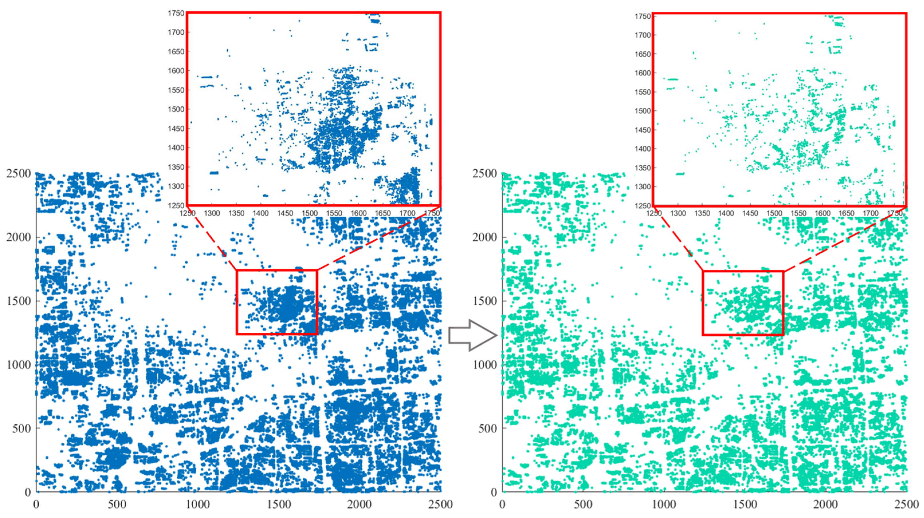
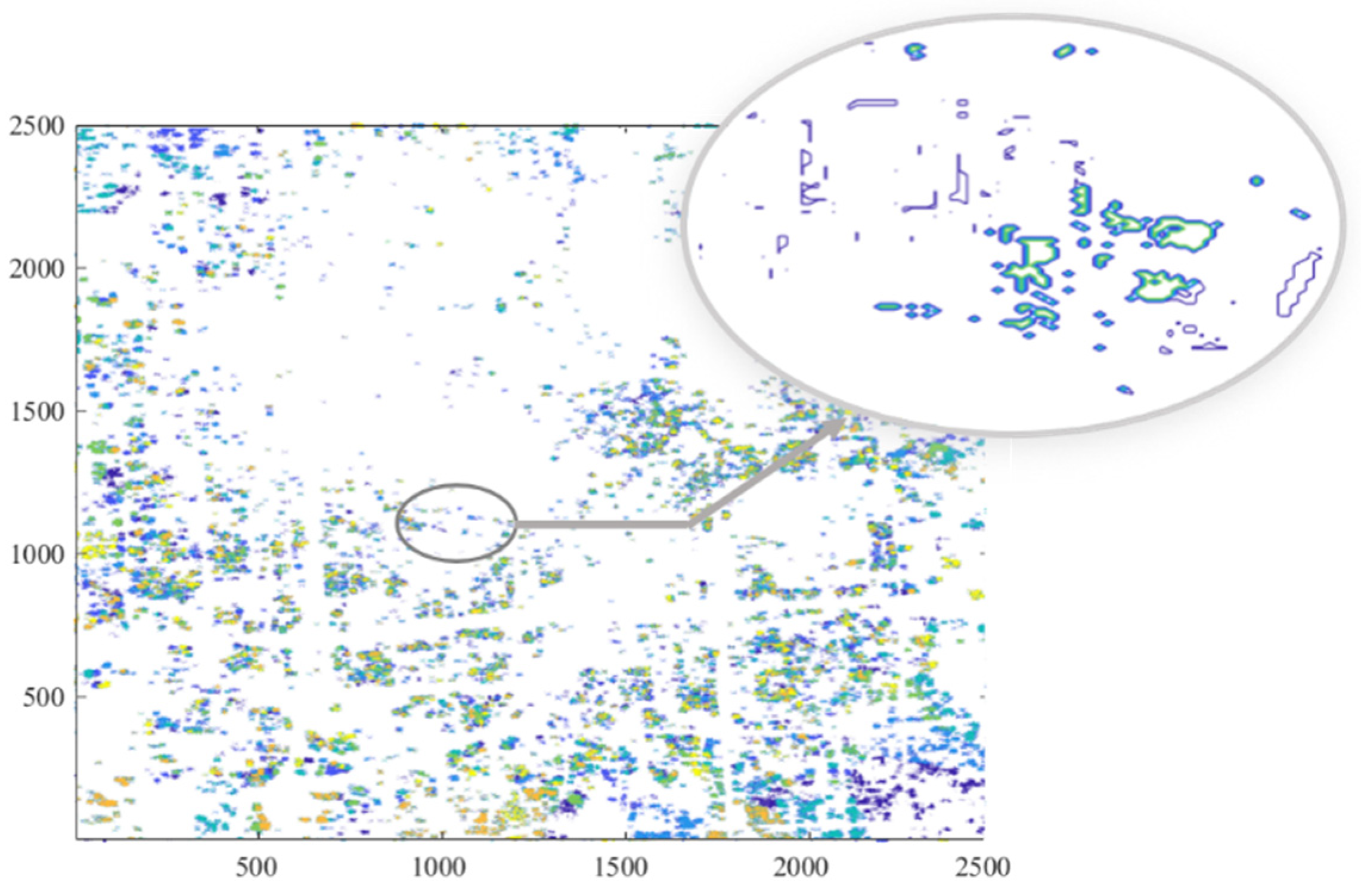
After several calculation attempts, the weak coverage points with service value lower than four were finally filtered as “noise points” in this paper. The comparison of weak coverage points before and after data processing is shown in Figure 1. After the above data preprocessing, the number of weak coverage points were reduced from the initial 182,807 to 83,841.

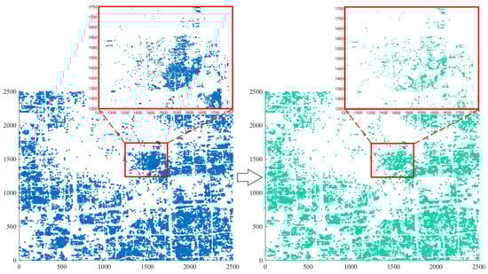
Figure 1. Comparison diagram of weak coverage point distribution before and after deleting “noise” points.

4. Methodology

Factors to be determined in base station construction planning mainly include three aspects: (1) coordinates of the site where the base station needs to be constructed; (2) the type of base station to be built; and (3) orientation of the three sectors of each base station. Considering that the judgment of the base station sector orientation is more complex than determining the base station type and location, two models were established in this paper to conduct a comparative study on this problem: (1) the location and type decision model of a single base station with circular coverage area and (2) the base station orientation decision model based on a “shamrock” shaped coverage area.

4.1. Decision Model of a Single Base Station with Circular Coverage Area

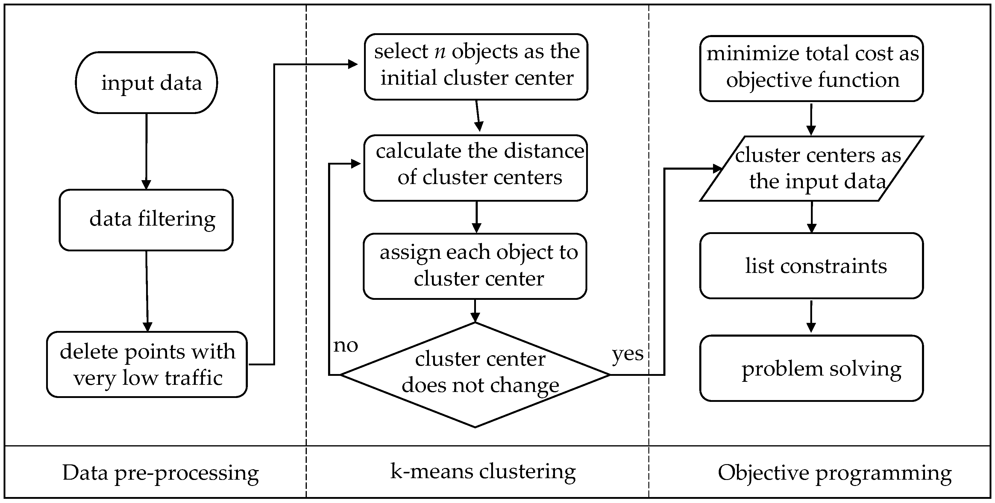
In this paper, the k-means clustering algorithm [27] was adopted to group the discrete weak coverage points and gather the small-scale weak coverage areas. The schematic diagram of 0–1 clustering planning model used in this paper is shown in Figure 2.

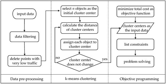
Figure 2. Schematic diagram of 0–1 clustering planning.

4.1.1. Classification of Weak Coverage Data Sets by k-Means Clustering Algorithm

As shown in Figure 2, the main steps of k-means clustering algorithm are: setting the number of groups n that you want to divide all data into; selecting n objects as the initial cluster center; calculating the distance from each object to each cluster center; and assigning each object to its nearest cluster center. At the same time, after each object is allocated, the cluster center will be re-determined, the final process is repeated until the set termination condition is satisfied.

(1)

Determining the number of required clustering centers

In this paper, the ratio of the number of weak coverage points to the total number of points in the distribution area was denoted as the distribution density of weak coverage points, expressed by ρ.

$$\rho =M/Z$$

(2)

where M represents the total number of weak coverage points and Z is the total number of weak coverage points in the distribution area. In reality, only when the distribution of the base station is not uniform will the weak coverage point appear. Therefore, the distribution area of weak coverage points needs to be divided separately. A more scientific approach is to gather all the circular areas with radius 30 around the weak coverage points into a total area so that the area with a good signal can be excluded. On this basis, all ranges with the coordinates of the old base station as the circle center and 30 as the radius were further excluded. In this way, the influence of the old base station on the weak coverage area can be eliminated. The range obtained by the final filtering is the area where the weak coverage points distribute. According to the above process, the calculation was carried out, the distribution area of weak coverage points obtained is shown in Figure 3.

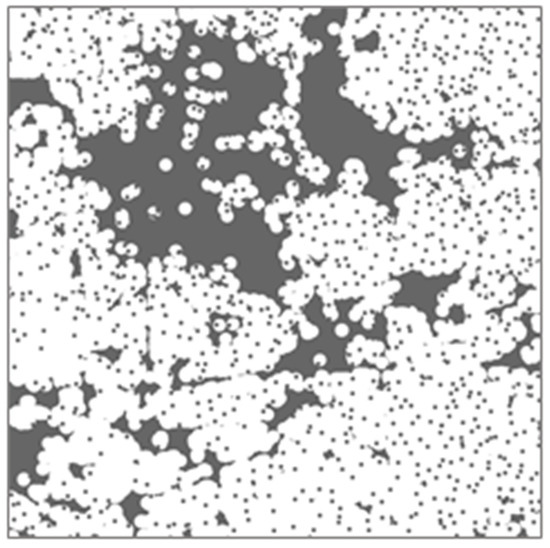
Figure 3. Distribution area of weak coverage points (the white area is weak coverage area).

The white area in Figure 3 represents the distribution area of weak coverage points, which contains 4,351,125 coordinate points. It is more accurate to calculate the distribution density of weak coverage points ρ by applying Equation (2).

After obtaining the distribution density of weak coverage points, it is necessary to estimate how many base stations are needed to cover all the weak coverage points evenly distributed in the region, under conditions of using both a micro base station with a radius of 10 and macro stations with a radius of 30. The calculation formula can be expressed as follows:

$$A=\frac{M}{S\times \rho }$$

(3)

where S represents the number of points that the base station can cover. The corresponding calculated average value of a micro base station is 317 and that of a macro base station is 2821. A indicates the number of base stations to be built. By substituting the existing data into the formula, we can get the number of two different types of base stations to be established. Then, we assign weights to the two types of base stations according to the actual situation. The number of clustering centers can be finally determined.

(2)

Clustering of weak coverage points

If the number of the k-means cluster is known, clustering can be implemented. MATLAB was used for programming calculation. The clustering distribution results obtained by classification is shown in Figure 4. The clusters of points of different colors shown in the figure are weak coverage points assigned to a cluster.

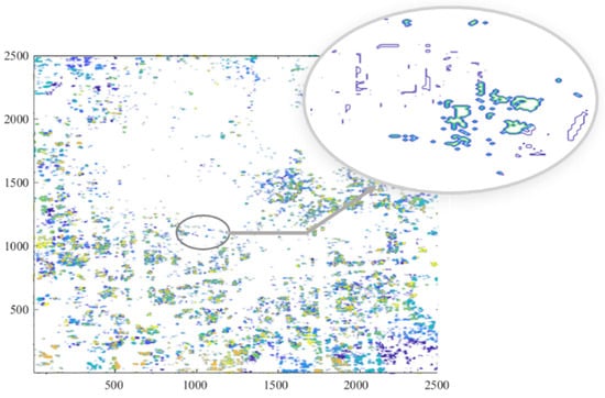
Figure 4. Distribution result of the weak coverage points after clustering.

4.1.2. Total Covered Business Amount of a Circular Coverage Area

After that, the problem was simplified to calculate the total traffic volume covered according to the site coordinates, quantity, and distribution of three known types of base stations (old base station, new micro and macro base stations). For different types of base stations, the method of calculating the coverage traffic is essentially the same. Taking the macro base station as an example.

Suppose that for a given macro station Z_i, its coordinates in Cartesian coordinates are (A_i, B_i), the weak coverage points in the circular coverage range are denoted as R_j(a_j, b_j). According to the Euclidean distance formula, the distance d_ij between the weak coverage point and the base station can be expressed as:

$$d_{ij}={\Vert Z_i-R_j\Vert }_2$$

(4)

Obviously, when the radius is greater than the distance between the weak coverage point and the base station site, this point cannot be covered, and the coefficient of the weak coverage point was assigned to 0; otherwise, the coefficient was assigned to 1.

$$R_j=\{\begin{array}{l} 1 , d_{ij}\le R\\ 0 , d_{ij}>R\end{array}$$

(5)

Therefore, by summing all the business volume y_j covered by the base station numbered j, the total business volume S_j covered by all macro base stations can be obtained.

$$S_j={\displaystyle \sum _{j=1}^n{R}_j\cdot y_j}$$

(6)

Similarly, for the micro base station, the only difference is that the coverage radius of the micro base station is 1, while that of the macro station is 10. The total business volume S_k covered by all base stations can also be obtained.

4.1.3. Establishment of Single-Objective Nonlinear Programming Model

In this paper, the single-objective nonlinear programming model was used to determine the site deployment by which the theoretical global optimal solution can be obtained.

(1)

Determination of objective function

Obviously, construction planning belongs to the planning model involving cost; the most common objective function for this type of question is to minimize the cost, while satisfying all constraints. Therefore, the objective function set in this paper is:

$$\mathrm{Min} W=\left\{10{\displaystyle \sum _{i=0}^n{a}_i}+{\displaystyle \sum _{i=0}^n{b}_i}\right\}$$

(7)

where W represents the total cost of building new base stations; a_i represents the situation of constructing macro station in the location with series number as i; b_i refers to the construction of micro-base station at the location with series number as i.

(2)

Determination of the constraints

After confirming the coordinates of points that can establish a base station, three situations need to be discussed for each point: don’t build a base station, build a micro base station, or build a macro base station. If a_i represents the 0–1 variable of a coordinate point to build a macro station; b_i represents the 0–1 variable of a coordinate point to build a micro base station. The 0~1 constraint can be expressed as follows:

$$\{\begin{array}{l}{a}_i=0,1\\ b_i=0,1\\ a_i+b_i\le 1\end{array}$$

(8)

In the meantime, the distance between different planned construction base stations should also be limited to avoid overlapping coverage. A_m is used to represent the location of the new base station with series number m; A_n represents the location of the new base station with series number n; and the distance constrain can be written as follows:

$${\Vert A_m-A_n\Vert }_2>10$$

(9)

Finally, it is necessary to ensure that the signal area covers at least 90% of the total business volume. The constraint of business volume can be expressed as:

$${\displaystyle \sum _{i=0}^n{\displaystyle \sum _{j=0}^n{S}_j\cdot a_i}+{\displaystyle \sum _{i=0}^n{\displaystyle \sum _{k=0}^n{S}_k\cdot b_i}}+P_o\ge 0.9\times P_t}$$

(10)

in which P_t represents the total business volume and P_o represents the sum of all the business volume covered by the old base station.

4.1.4. Final Single-Objective Programming Model Based on Circular Coverage Area

Finally, by taking the total cost of constructing new base stations as the objective function, the 0–1 constraint to limit one base station built in each point, the distance between adjacent base stations is bigger than 10, and the signal area covering at least 90% of the traffic as the constraint conditions. A single-objective nonlinear programming model can be established as follows.

$$\mathrm{Min} W=\left\{10{\displaystyle \sum _{i=0}^n{a}_i}+{\displaystyle \sum _{i=0}^n{b}_i}\right\}$$

subject to (8)–(10).

4.2. Base Station Orientation Decision Model Based on “Shamrock” Coverage Area

In fact, the signal coverage of each base station is not circular. Most base stations have three sectors, each pointing in different directions. The sector has the farthest signal coverage distance in the main direction. It can be covered in a certain range around the main direction, but the coverage gradually decreases with the angle according to a certain law. In this paper, it is assumed that the coverage of the area around the main direction of 60° attenuates to approximately 75% of the maximum range. At the same time, considering the utilization of coverage, generally, the included angle between the main direction should be not less than 45° for any two “blades” of the same base station.

In order to determine the main direction orientation of the “shamrock” blade, three angle variables need to be introduced. Therefore, the polar coordinate system obviously has great advantages compared with the Cartesian coordinate system in the model establishment. Considering the huge number of base stations to be established in this paper, a polar coordinate system set was finally established, the poles of each polar coordinate system fall on the coordinates of the site where the base station is to be established. Subsequent discussions were taken at each polar coordinate system of each coordinate system set.

4.2.1. Proposed “Shamrock” Shaped Coverage Area Model

(1)

Introduction of the area covered by the “shamrock” model

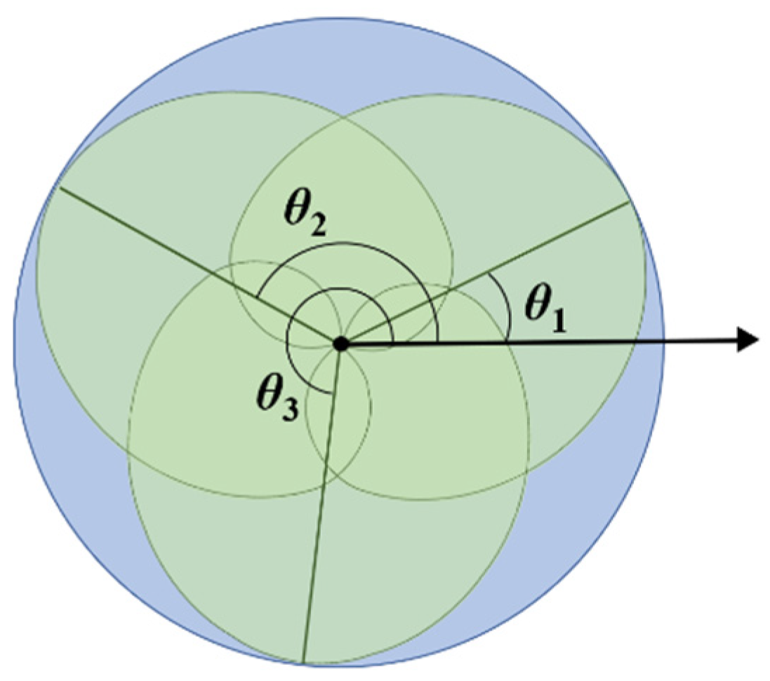
According to the previous description as well as the established polar coordinate system, a schematic diagram of the “shamrock” shaped coverage area is shown in Figure 5.

Figure 5. Schematic diagram of the “shamrock” covering model built in polar coordinate system.

The figure above shows a particular state of the “shamrock” coverage area combined with polar coordinates. The light blue circle area represents the traditional circular coverage area. The “shamrock” shaped coverage area is colored in light green. Different lines indicate the direction of the center of each sector. The three angles represent the rotation angle of each sector based on polar coordinates. It can be seen there are great differences in coverage areas between the two different models.

In this case, by determining the rotation angle of each sector at a particular pole, the state of the area covered by that pole can be obtained. Meanwhile, in order to ensure that the included angle between the main directions of each two sectors is not less than 45°, the following constrain should be met:

$$\{\begin{array}{l}{\theta }_2-{\theta }_1>{45}^{\circ }\\ {\theta }_3-{\theta }_2>{45}^{\circ }\\ {\theta }_3-{\theta }_2<{315}^{\circ }\end{array}$$

(11)

Meanwhile, the relation between the real coverage area of a base station and the angle change value can be approximated as a heart-shaped line. Assuming the radius is ρ, the coverage area of any sector can be expressed in the following formula according to polar coordinates, where θ₀ represents the angle of a sector with polar axis rotation:

$$\rho =\frac{2\arctan \left|\theta \right|+\pi }{\pi }\left[1+\cos \left({\theta }_0-\theta \right)\right]·R$$

(12)

(2)

Simplify data by analyzing coverage areas

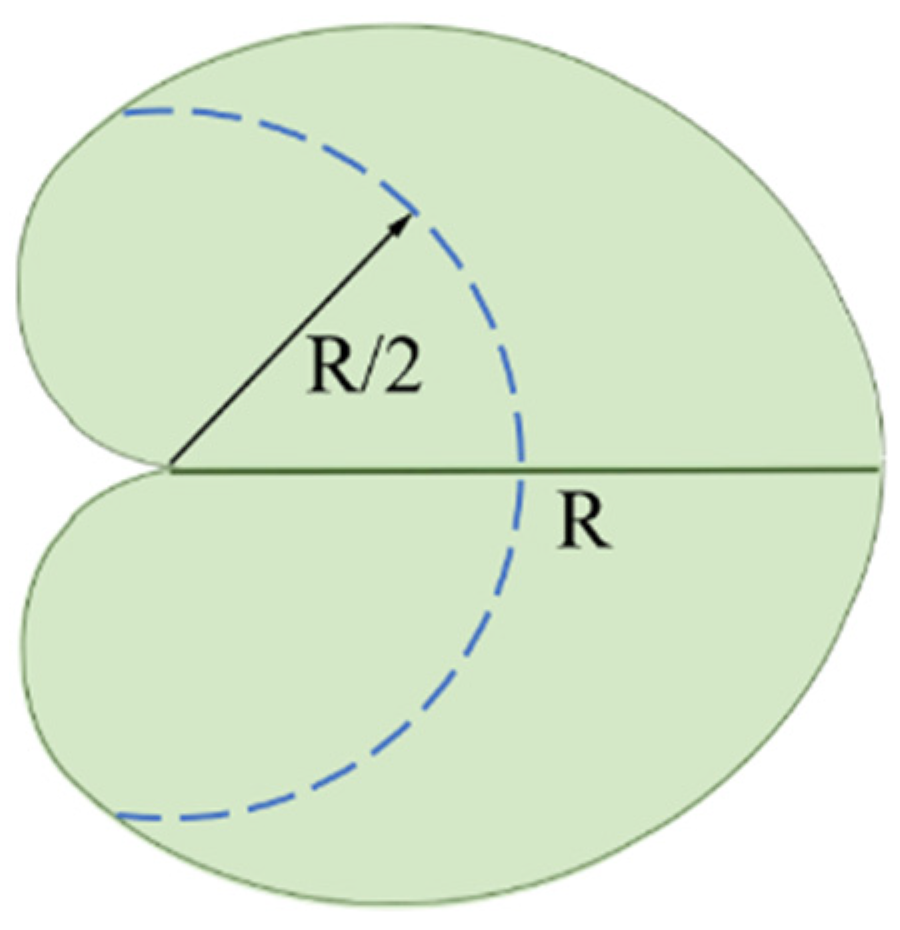
The details for a sector of any “shamrock” shaped coverage area are shown in Figure 6:

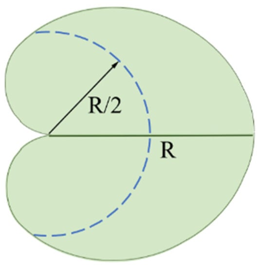
Figure 6. Detail of a sector of the “shamrock” shaped coverage area.

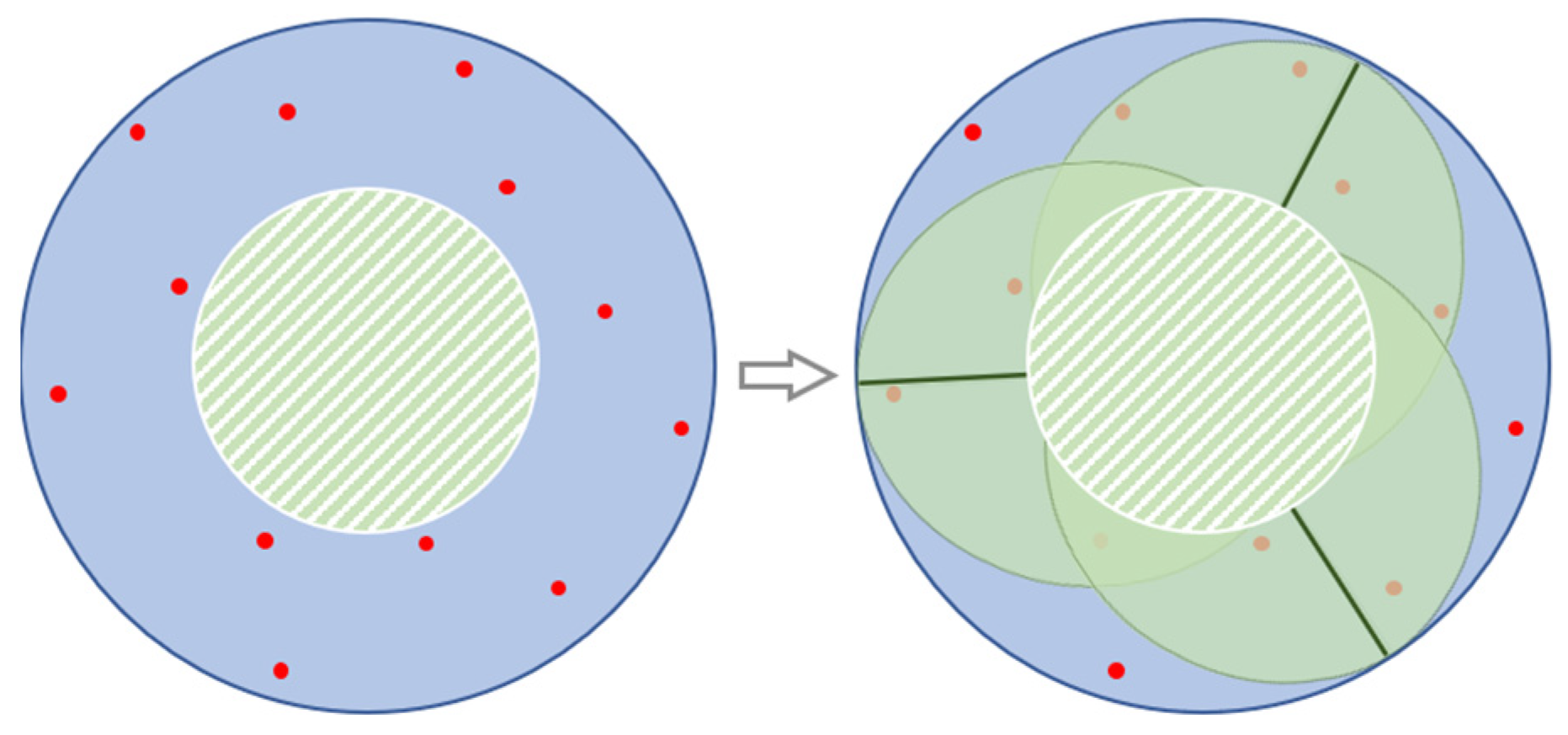
It can be seen from Figure 6 that in any case, a sector of 120° radian with radius R/2 can always be guaranteed to be fully covered. At the same time, under the given constraints, the three sectors of each base station will overlap, resulting in the central area also being affected by overlap. However, considering that the purpose of each base station is to cover as much business volume as possible, different sectors are distributed relatively evenly in most cases so that the area with R/2 radius as the center of each base station can be completely covered, as the shadow area shown in Figure 7:

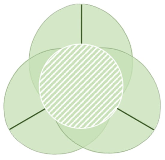
Figure 7. Idealized signal coverage diagram.

In the subsequent calculation, by default, for all base stations, it is regarded that the weak coverage points with a Euclidean distance less than R/2 can be fully covered. In this way, the number of weak coverage points needs to be discussed as they can be reduced theoretically, and the spatial complexity of the model can be greatly reduced.

(3)

Determination of the main direction based on k-means clustering algorithm

According to the analysis above, the problem has been simplified to cover as many weak coverage points in the ring region as possible. A schematic diagram is shown in Figure 8.

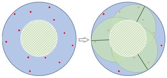
Figure 8. Schematic diagram of a ring signal cover region.

In order to determine the main directions of the three sectors and to cover as many points as possible, the k-means clustering algorithm was used again to separate all points according to the pole angle of the polar coordinate system. The number of cluster centers selected for this division was three.

It is assumed that the coordinates of the clustering center point obtained after calculation are M_m (a_i, b_i). Then, this point was connected to the coordinates of base station N_n (A_i, B_i); the obtained line direction is the main direction. The transformation formula can be obtained from the relation between the Cartesian coordinate and polar coordinate angle. θ_i was used to represent the polar coordinate angle of the “blade” with series number i in a “shamrock” model; the transformation formula can be written as follows:

$$\begin{array}{l}\{\begin{array}{l}{\theta }_i{}^{\prime }=\arctan \left(\frac{\left|b_i-B_i\right|}{\left|a_i-A_i\right|}\right)\\ {\theta }_i=\{\begin{array}{l}{\theta }_i{}^{\prime } , a_i>A_i,b_i>B_i\\ \pi -{\theta }_i{}^{\prime } , a_i>A_i,b_i<B_i\\ \pi +{\theta }_i{}^{\prime } , a_i<A_i,b_i<B_i\\ 2\pi -{\theta }_i{}^{\prime } , \mathrm{else}\end{array}\end{array}\\ \end{array}$$

(13)

For each base station, the clustering center coordinates of the three ring weak coverage points obtained by the k-means algorithm were substituted into the above formula, the optimal coverage distribution state of each base station after changing the shape of the coverage range could be obtained.

4.2.2. Solution of the Total Amount of Covered Business

According to Formula (13), the deflection angle of the weak coverage point in the polar coordinate system θ_ij can be written as:

$$\begin{array}{l}\{\begin{array}{l}{\theta }_i{}^{\prime }=\arctan \left(\frac{\left|b_j-B_i\right|}{\left|a_j-A_i\right|}\right)\\ {\theta }_{ij}=\{\begin{array}{l}{\theta }_i{}^{\prime } , a_j>A_i,b_j>B_i\\ \pi -{\theta }_i{}^{\prime } , a_j>A_i,b_j<B_i\\ \pi +{\theta }_i{}^{\prime } , a_j<A_i,b_j<B_i\\ 2\pi -{\theta }_i{}^{\prime } , \mathrm{else}\end{array}\end{array}\\ \end{array}$$

(14)

According to Formula (12), the radius length ρ corresponding to a specific angle in any sector can be determined by the formula:

$$\rho =\{\begin{array}{l}\left(1-\frac{3{\theta }_0}{2\pi }\right)·R+\frac{3R}{2\pi }·{\theta }_{ij}, {\theta }_0-\frac{\pi }{3}\le {\theta }_{ij}<{\theta }_0\\ \left(1+\frac{3{\theta }_0}{2\pi }\right)·R-\frac{3R}{2\pi }·{\theta }_{ij}, {\theta }_0\le {\theta }_{ij}<{\theta }_0+\frac{\pi }{3}\end{array}$$

(15)

For a macro base station, it is the same as the circular coverage area, according to the Euclidean distance formula, the distance $d_{ij}^{\prime }$ between the weak coverage point and the base station can be expressed as:

$$d_{ij}^{\prime }={\Vert Z_i^{\prime }-R_j^{\prime }\Vert }_2$$

(16)

Obviously, when the radius of the blade is greater than the distance between the weak coverage point and the base station site, the point cannot be covered, and the value of R’_j is assigned to 0. Otherwise, it is assigned to 1.

$$R_j^{\prime }=\{\begin{array}{l} 1 , d_{ij}\le \rho \\ 0 , d_{ij}>\rho \end{array}$$

(17)

Therefore, by summing all the business volume $y_j^{\prime }$ covered by the base station numbered j, the total business volume $S_j^{\prime }$ covered by all macro base stations can be obtained.

$$S_j^{\prime }={\displaystyle \sum _{j=1}^n{R}_j^{\prime }·y_j^{\prime }}$$

(18)

Similarly, for the micro base station, the total business volume $S_k^{\prime }$ covered by all base stations can also be obtained.

4.2.3. Improved Model with Considering the Coverage Domain Overlap

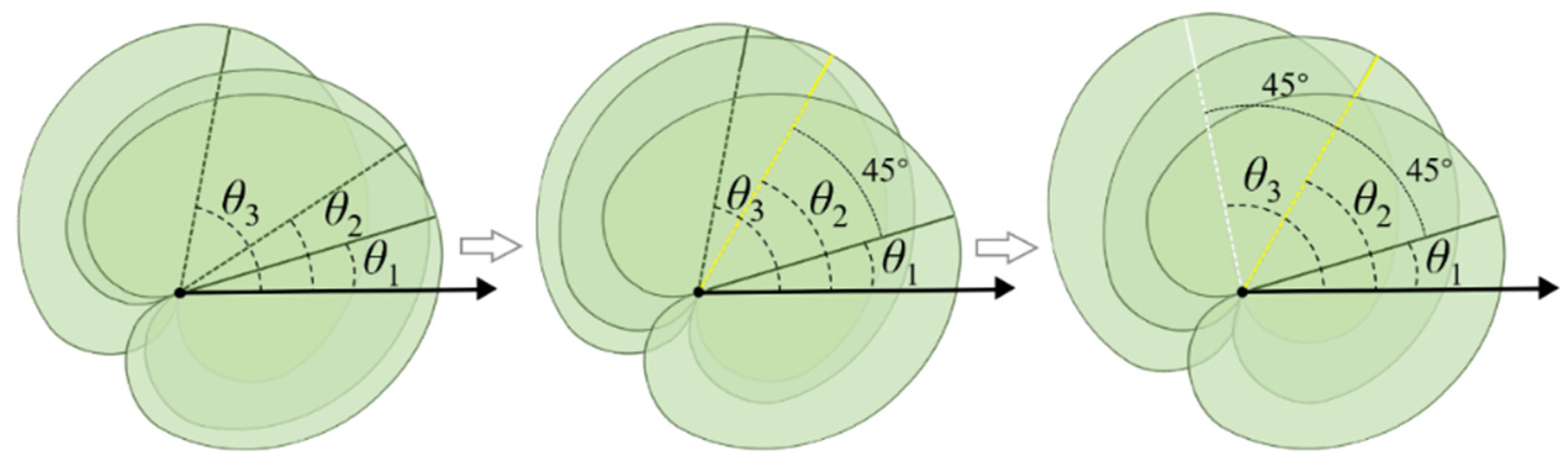
After completing all the steps above, the model in this paper has basically realized the judgment of the sector orientation; but, in an actual situation it is necessary that the angle between the main directions of any two sectors not be less than 45°. In this paper, all sectors of a coverage area were numbered as 1, 2, and 3 in the counterclockwise direction. When considering the angle in the main direction, we need only to consider the angle between 1–2, 2–3, and 3–1. It is assumed in this paper that if the detected angle between the main direction is less than 45°, the former of the two sectors should be fixed and its angle remain unchanging, the angle increased to the critical condition by rotating the latter angle. At the same time, for the second blade, if the changing of the angle leads to the angle between the second and the third sectors being less than 45°, these two blades were gathered into a new group and the above operations were repeated. Obviously, the most extreme case of each “shamrock” requires only two rotations of the blades, as shown in Figure 9:

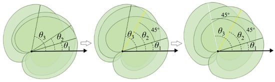
Figure 9. Illustration of extreme case correction.

Based on the above analysis, the formula of a regional overlap modification model can be expressed as:

$$\{\begin{array}{l}{\theta }_2={\theta }_1+\pi /4, \left|{\theta }_2-{\theta }_1\right|<\pi /4\\ {\theta }_3={\theta }_2+\pi /4, \left|{\theta }_3-{\theta }_2\right|<\pi /4\\ {\theta }_1={\theta }_3+\pi /4, \left|{\theta }_1-{\theta }_3\right|<\pi /4\end{array}$$

(19)

Using the above method, the coverage area of the base station can be modified. Eventually, all base station coverage can be changed to a realistic “shamrock” state.

4.2.4. Decision by Using Single-Objective Nonlinear Programming Model

The same as the model built for a circular coverage area, a single-objective nonlinear programming model can also be established for “shamrock” shaped areas.

The objective function established was:

$$\mathrm{Min} W{}^{\prime }=\left\{10{\displaystyle \sum _{i=0}^n{a}_i^{\prime }}+{\displaystyle \sum _{i=0}^n{b}_i^{\prime }}\right\}$$

(20)

where W′ represents the total cost of building new base stations; $a_i^{\prime }$ represents the situation of constructing a macro station in the location with a series number as i; and $b_i^{\prime }$ refers to the construction of a micro-base station at the location with a series number as i. All constraints can be determined as:

Judging whether to build base station and the type of base station to be built:

$$\{\begin{array}{l}{a}_i^{\prime }=0,1\\ b_i^{\prime }=0,1\\ a_i^{\prime }+b_i^{\prime }\le 1\end{array}$$

(21)

Constrain used to avoid overlapping coverage:

$${\Vert A_m^{\prime }-A_n^{\prime }\Vert }_2>10$$

(22)

Constraints on region overlap modification:

$$\{\begin{array}{l}{\theta }_2={\theta }_1+\pi /4, \left|{\theta }_2-{\theta }_1\right|<\pi /4\\ {\theta }_3={\theta }_2+\pi /4, \left|{\theta }_3-{\theta }_2\right|<\pi /4\\ {\theta }_1={\theta }_3+\pi /4, \left|{\theta }_1-{\theta }_3\right|<\pi /4\end{array}$$

Also, to ensure that the signal area covers at least 90% of the total business volume:

$${\displaystyle \sum _{i=0}^n{\displaystyle \sum _{j=0}^n{S}_j^{\prime }·a_i^{\prime }}+{\displaystyle \sum _{i=0}^n{\displaystyle \sum _{k=0}^n{S}_k^{\prime }·b_i^{\prime }}}+P_o\ge 0.9\times P_t}$$

(23)

4.2.5. Final Model Based on “Shamrock” Shaped Coverage Area

Finally, for the “shamrock” shaped coverage area, the single-objective nonlinear programming model can be established as follows.

$$\mathrm{Min} W{}^{\prime }=\left\{10{\displaystyle \sum _{i=0}^n{a}_i^{\prime }}+{\displaystyle \sum _{i=0}^n{b}_i^{\prime }}\right\}$$

subject to Equations (19), (21)–(23).

For this proposed model, the objective function and the constraints are very clear. The commercial optimization modelling software, LINGO 18, can be used to find the optimal layout scheme and the least cost.

5. Results and Discussion

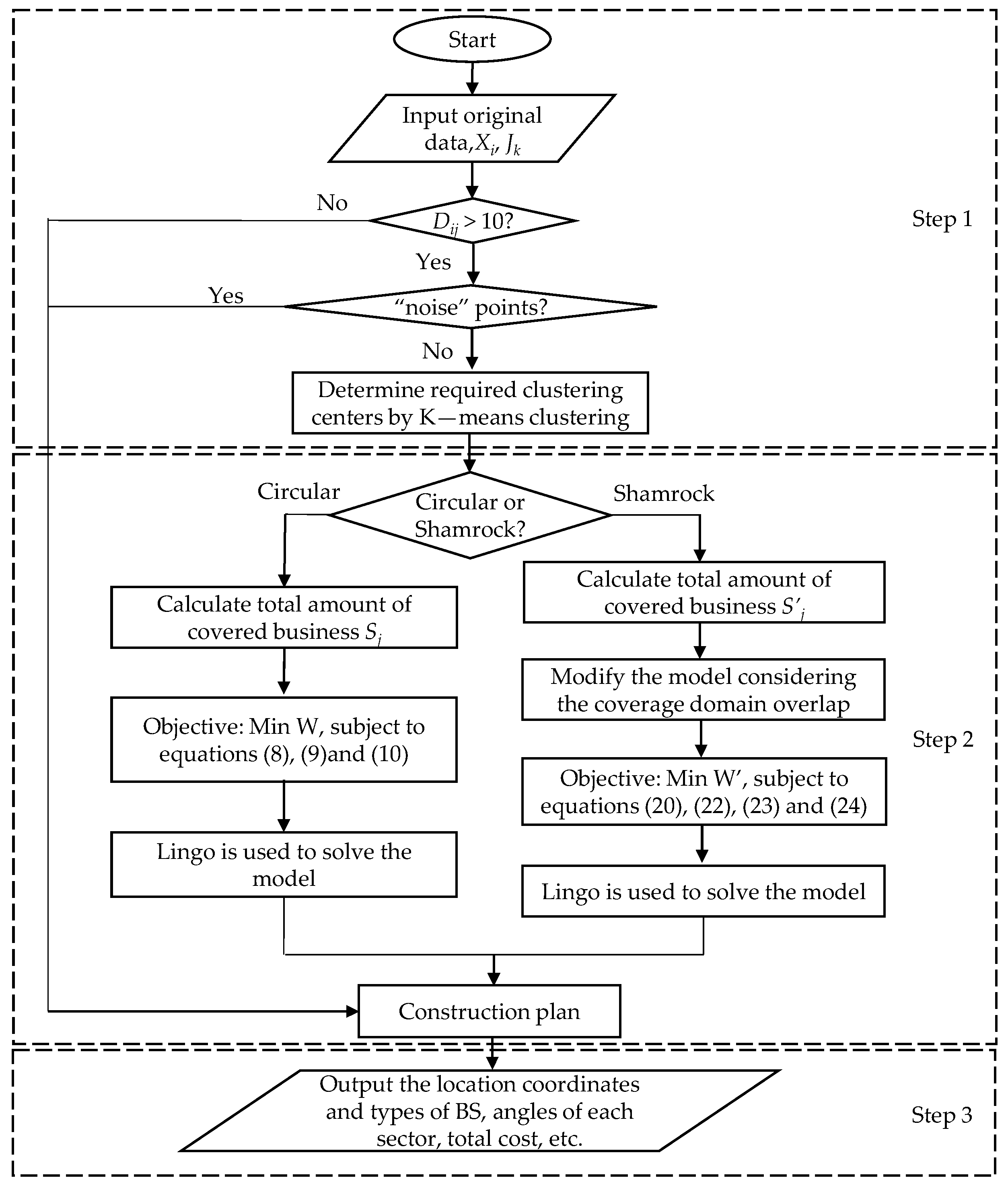
A flow chart of planning the base station is shown in Figure 10. The whole solving process of this paper can be divided into three main steps: (1) data preprocessing and K-means clustering by using MATLAB software; (2) based on the data processed by MATLAB, LINGO was used for the programming solution to obtain the minimum cost and the location of the base station, two different approaches based on the circular and the “shamrock” shaped coverage areas were presented, respectively; and (3) according to the results of LINGO, MATLAB was used again to draw the position of the base station in the region to be planned.

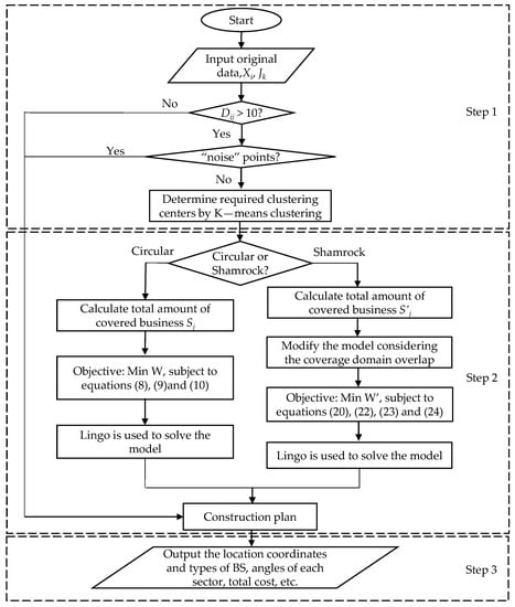
Figure 10. Flow chart of proposed algorithm.

5.1. Solution of Single Base Station with Circular Coverage Area

Based on the single-objective linear programming model established in Section 4.1 (Equations (7)–(10)) as well as the flow chart shown in Figure 10, the optimal layout scheme and the least cost can be calculated. According to the result, 8856 micro base stations are to be built and the number of macro stations is 412, which covers 6,599,691 businesses and accounts for 93.53% of the total business volume, the nominal cost is 10,092.

For a detailed construction plan, it is necessary to determine the coordinates and types of base stations to be constructed. Considering the huge amount of data, only 20 results are listed in this paper, as shown in Table 2.

Table 2. Part results of the location coordinates and types of base stations needed to be established.

Series Number	X Coordinates	Y Coordinates	Type	Series Number	X Coordinates	Y Coordinates	Type
1	1985	1495	Micro BS	11	493	629	Micro BS
2	1662	1191	Micro BS	12	540	438	Micro BS
3	1501	1501	Micro BS	13	1641	1153	Micro BS
4	1532	241	Micro BS	14	1836	1331	Micro BS
5	218	2328	Micro BS	15	158	929	Micro BS
6	1009	1009	Micro BS	16	168	2006	Micro BS
7	1228	963	Macro BS	17	555	282	Micro BS
8	1864	1528	Micro BS	18	1733	656	Micro BS
9	602	1024	Micro BS	19	1637	667	Macro BS
10	914	671	Micro BS	20	1867	1325	Micro BS

5.2. Solution Based on “Shamrock” Shaped Coverage Area Model

Similarly, according to Equations (19)–(23) as well as the flow chart shown in Figure 10, it can be obtained that a total of 9043 micro base stations and 437 macro stations need to be established, which covers 6,499,493 businesses and accounts for 92.11% of the total business volume, the total nominal cost is 10,530. Results of 10 base stations are listed in Table 3.

Table 3. Part results of the location coordinates and types of base stations needed to be established.

Serial Number	X Coordinates	Y Coordinates	Type	θ1	θ2	θ3
1	309	1486	Micro BS	42°	148°	284°
2	77	1299	Micro BS	17°	151°	240°
3	1905	127	Micro BS	103°	228°	324°
4	2464	1539	Micro BS	95°	197°	282°
5	1063	438	Micro BS	51°	166°	268°
6	1838	1838	Micro BS	7°	133°	226°
7	2338	741	Micro BS	22°	152°	248°
8	2212	1062	Macro BS	65°	165°	255°
9	1889	2420	Micro BS	26°	142°	234°
10	1955	128	Micro BS	49°	133°	267°

It can be seen from Table 3 that based on the proposed model, both the coordinates and the angles of all sectors can be obtained.

5.3. Discussion

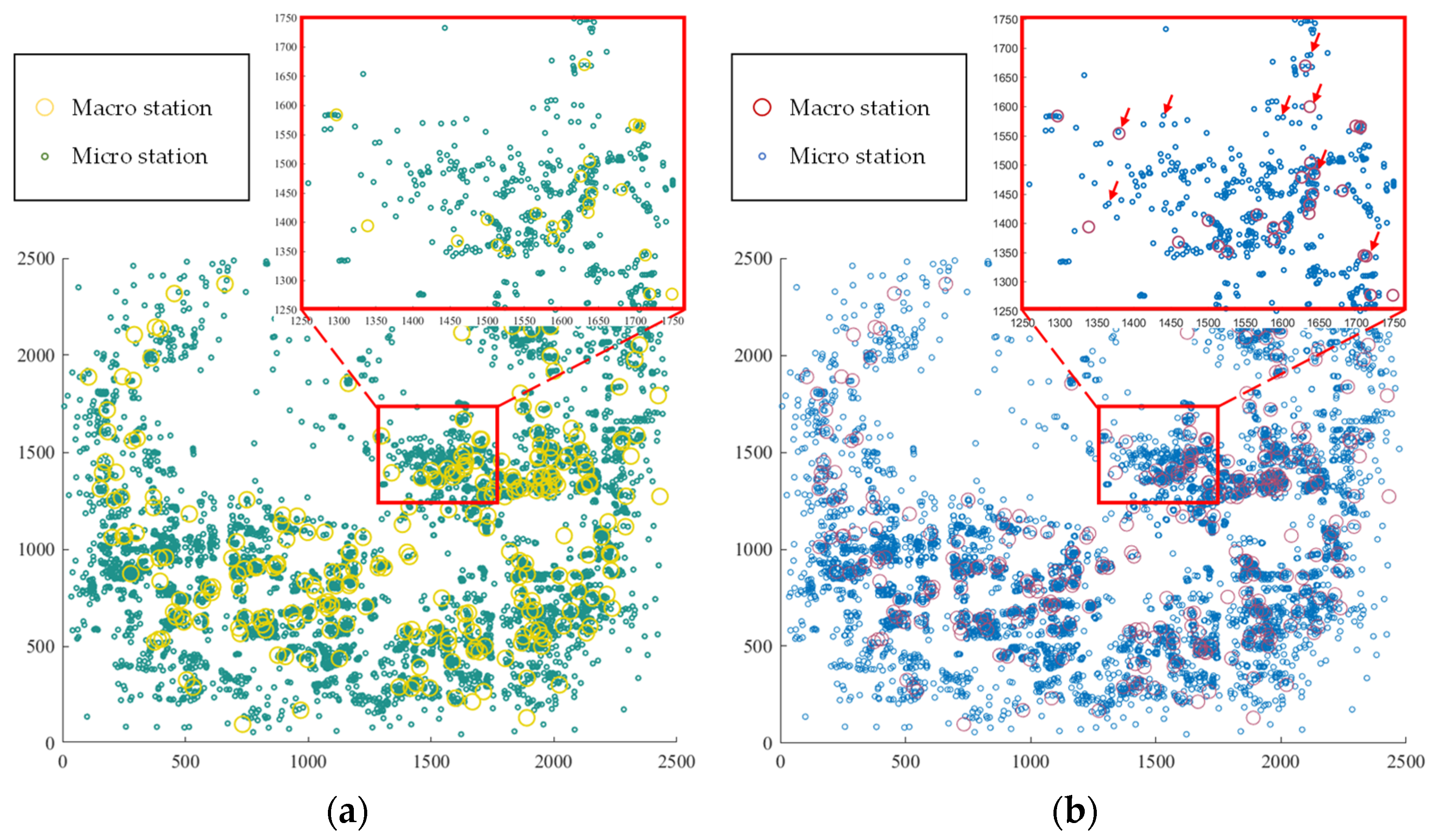
According to the above method, the optimal plannings of base station construction for both circular and “shamrock” shaped coverage areas were calculated, respectively, the comparison results are shown in Figure 11.

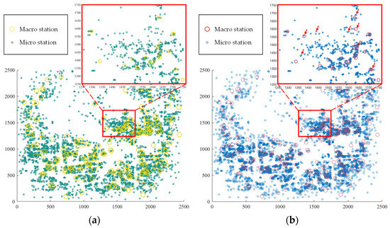
Figure 11. Diagrams showing the locations and the types of base stations need to be constructed. (a) shows— the results based on a circular coverage area, the big circles with ochre yellow are the macro stations, and the dark green circles are the positions of the micro stations. (b) shows the results based on the “shamrock” shaped coverage area, the big red circles are the macro stations and the blue circles are the positions of the micro stations. The red arrows in the zoom window shows part of the differences compared with the corresponding positions in (a).

For the results based on a circular coverage area, the number of macro stations needed to be built is 8856, the number of micro stations is 412, and the nominal cost is 10,092. For the results based on the “shamrock” shaped coverage area, the numbers of macro and micro stations are 9102 and 476, respectively, and the total nominal cost is 10,530.

According to the results of the two methods, it can be found that the number of base station planning using the “shamrock” shaped coverage area algorithm increased slightly, and it results in a slight increase in cost compared with the circular coverage area. However, since the two coverage models have very different coverage areas, the improved “shamrock” model proposed in this paper can effectively reduce the occurrence of repeated coverage, which is also more reasonable.

6. Conclusions

Firstly, the complexity of calculation is configurable by multi-step data filtering. The stepwise design of the model greatly improves the degree of flexibility. The available scenarios of the model can be broadened by adjusting parameters, which also makes the adjustment of the model more convenient.

Secondly, in order to get closer to reality, the “shamrock” shaped of the coverage area model was used in comparison with the circular coverage area model. When determining the sector orientation of the “shamrock” coverage area model, a k-means clustering algorithm was introduced again in a small range. These changes make the planning of base station construction more reasonable with the observation that the final signal coverage is more uniform and the overlapping waste of signal coverage domain is reduced.

Thirdly, single-objective nonlinear programming was used to plan the base station construction. This method permits finding the global optimal solution theoretically, but the disadvantage is the excessive demand on computing power. The model used in this paper can be further extended to a multi-objective function so that more evaluation indicators can be taken into account; the model will be much closer to the real situation.

Finally, some factors related to propagation, such as shadowing or effects related to antenna radiation patterns, were not taken into account in this paper, which can have a detrimental effect on coverage in certain points. These factors are left for future study.

This model is mainly based on clustering of a large dataset sample and optimization based on density distribution for resource allocation problems. Although the capacity of the model is manifested by the special case of the base station construction planning, theoretically, this model can also be used to solve various problems related to dynamic resource allocation regulation with a wide range of application scenarios.

References

- Cantlebary, L.; Li, L. Facility Location Problem. Available online: https://optimization.cbe.cornell.edu/index.php?title=Facility_location_problem (accessed on 20 May 2022).
- Mathar, R.; Niessen, T. Optimum Positioning of Base Stations for Cellular Radio Networks. Wirel. Netw. 2000, 6, 421–428. [Google Scholar] [CrossRef]
- MathorCup-University Mathematical Modeling Competition, Question 2022D. Chinese Society of Optimization, Overall Planning and Economic Mathematics. Available online: http://mathorcup.org/detail/2378 (accessed on 20 May 2022).
- Mathar, R.; Schmeink, M. Optimal Base Station Positioning and Channel Assignment for 3G Mobile Networks by Integer Programming. Ann. Oper. Res. 2001, 107, 225–236. [Google Scholar] [CrossRef]
- Zimmermann, J.; Höns, R.; Mühlenbein, H. ENCON: An evolutionary algorithm for the antenna placement problem. Comput. Ind. Eng. 2003, 44, 209–226. [Google Scholar] [CrossRef]
- Amaldi, E.; Capone, A.; Malucelli, F.; Signori, F. Radio Planning and Optimization of W-CDMA Systems. In Proceedings of the 2003 International Federation for Information Processing, Venice, Italy, 23–25 September 2003; Volume 2775, pp. 437–447. [Google Scholar]
- Amaldi, E.; Capone, A.; Malucelli, F. Planning UMTS Base Station Location: Optimization Models with Power Control and Algorithms. IEEE Trans. Wirel. Commun. 2003, 2, 939–952. [Google Scholar] [CrossRef]
- Amaldi, E.; Capone, A.; Malucelli, F. Radio Planning and Coverage Optimization of 3G Cellular Networks. Wirel. Netw. 2008, 14, 435–447. [Google Scholar] [CrossRef]
- Amaldi, E.; Capone, A.; Malucelli, F.; Mannino, C. Optimization Problems and Models for Planning Cellular Networks. In Handbook of Optimization in Telecommunications; Springer: Berlin/Heidelberg, Germany, 2006. [Google Scholar]
- Khalek, A.A.; Ai-Kanj, L.; Zaher, D.; Turkiyyah, G. Site Placement and Site Selection Algorithms for UMTS Radio Planning with Quality Constraints. In Proceedings of the 2010 International Conference on Telecommunications, Doha, Qatar, 4–7 April 2010; pp. 375–381. [Google Scholar]
- Ibrahim, L.F.; Hamed, M.H. Using clustering technique M-PAM in mobile network planning. In Proceedings of the 12th WSEAS International Conference on Computers, Heraklion, Greece, 23–25 July 2008. [Google Scholar]
- Ibrahim, L.F.; Salman, H.A. Using Hyper Clustering Algorithms in Mobile Network Planning. Am. J. Appl. Sci. 2011, 8, 1004–1013. [Google Scholar] [CrossRef]
- Mai, W.; Liu, H.; Chen, L.; Li, J.; Xiao, H. Multi-objective Evolutionary Algorithm for 4G Base Station Planning. In Proceedings of the 2013 International Conference on Computational Intelligence and Security, Emeishan, China, 14–15 December 2013; pp. 85–89. [Google Scholar]
- Selim, S.Z.; Almoghathawi, Y.A.; Aldajani, M. Optimal Base Stations Location and Configuration for Cellular Mobile Networks. Wirel. Netw. 2015, 21, 13–19. [Google Scholar] [CrossRef]
- Valavanis, I.; Athanasiadou, G.; Zarbouti, D.; Tsoulos, G.V. Multi-Objective Optimization for Base-Station Location in Mixed-Cell LTE Networks. In Proceedings of the 10th European Conference on Antennas and Propagation (EuCAP), Davos, Switzerland, 10–15 April 2016. [Google Scholar]
- Iellamo, S.; Lehtomaki, J.J.; Khan, Z. Placement of 5G Drone Base Stations by Data Field Clustering. In Proceedings of the 2017 IEEE Vehicular Technology Conference (VTC Spring), Sydney, Australia, 4–7 June 2017; pp. 1–5. [Google Scholar]
- Goudos, S.; Diamantoulakis, P.; Karagiannidis, G. Multi-objective Optimization in 5G Wireless Networks with Massive MIMO. IEEE Commun. Lett. 2018, 22, 2346–2349. [Google Scholar] [CrossRef]
- Wang, C.H.; Lee, C.J.; Wu, X. A Coverage-Based Location Approach and Performance Evaluation for the Deployment of 5G Base Stations. IEEE Access 2020, 8, 123320–123333. [Google Scholar] [CrossRef]
- Fraiha, R.; Gomes, I.; Gomes, C.; Gomes, H.; Cavalcante, G. Improved Multi-objective Optimization for Cellular Base Stations Positioning. Journal of Microwaves. Optoelectron. Electromagn. Appl. 2021, 20, 870–882. [Google Scholar]
- Gomes, C.; Gomes, I.; Fraiha, R.; Gomes, H.; Cavalcante, G. Optimum Positioning of Base Station for Cellular Service Devices Using Discrete Knowledge Model. J. Microwaves. Optoelectron. Electromagn. Appl. 2020, 19, 428–443. [Google Scholar] [CrossRef]
- Liang, M.; Li, W.; Ji, J.; Zhou, Z.; Zhao, Y.; Zhao, H.; Guo, S. Evaluating the Comprehensive Performance of 5G Base Station: A Hybrid MCDM Model Based on Bayesian Best-Worst Method and DQ-GRA Technique. Math. Probl. Eng. 2022, 2022, 4038369. [Google Scholar] [CrossRef]
- Liu, J.; Ting, S.; Sarkar, T. Base-station Antenna Modeling for Full-wave Electromagnetic Simulation. In Proceedings of the 2014 IEEE International Symposium on Antennas and Propagation & USNC/URSI National Radio Science Meeting, Memphis, TN, USA, 6–11 July 2014; pp. 2106–2107. [Google Scholar]
- Blanch, S.; Romeu, J.; Cardama, A. Near Field in the Vicinity of Wireless base-station Antennas: An Exposure Compliance Approach. IEEE Trans. Antennas Propag. 2002, 50, 685–692. [Google Scholar] [CrossRef]
- Wu, C.H.; Yang, C.F.; Wang, T.S.; Liao, K.C.; Chen, Y.M. A Method to Improve the Radiation Patterns of the Base Station Sector Antenna for Mobile Communications by Adding Scattering Structures on the Front Panel of the Antenna. In Proceedings of the 2006 IEEE Antennas and Propagation Society International Symposium, Albuquerque, NM, USA, 9–14 July 2006; pp. 4357–4360. [Google Scholar]
- Konstantinidis, A.; Yang, K.; Zhang, Q. An Evolutionary Algorithm to a Multi-Objective Deployment and Power Assignment Problem in Wireless Sensor Networks. In Proceedings of the IEEE GLOBECOM 2008—2008 IEEE Global Telecommunications Conference, New Orleans, LA, USA, 30 November–4 December 2008; pp. 1–6. [Google Scholar]
- Khalily-Dermany, M. Transmission power assignment in network-coding-based-multicast-wireless-sensor networks. Comput. Netw. 2021, 196, 108203. [Google Scholar] [CrossRef]
- MacQueen, J. Some Methods for Classification and Analysis of Multivariate Observations. In Proceedings of the 5th Berkeley Symposium on Mathematical Statistics and Probability, Berkeley, CA, USA, 21 June–18 July 1965 and 27 December 1965–7 January 1966; Statistical Laboratory of the University of California: Berkeley, CA, USA, 1967; Volume 1, pp. 281–297. [Google Scholar]
Publisher’s Note: MDPI stays neutral with regard to jurisdictional claims in published maps and institutional affiliations. |
© 2022 by the authors. Licensee MDPI, Basel, Switzerland. This article is an open access article distributed under the terms and conditions of the Creative Commons Attribution (CC BY) license (https://creativecommons.org/licenses/by/4.0/).