Solving Inverse Conductivity Problems in Doubly Connected Domains by the Homogenization Functions of Two Parameters

Abstract

In the paper, we make the first attempt to derive a family of two-parameter homogenization functions in the doubly connected domain, which is then applied as the bases of trial solutions for the inverse conductivity problems. The expansion coefficients are obtained by imposing an extra boundary condition on the inner boundary, which results in a linear system for the interpolation of the solution in a weighted Sobolev space. Then, we retrieve the spatial- or temperature-dependent conductivity function by solving a linear system, which is obtained from the collocation method applied to the nonlinear elliptic equation after inserting the solution. Although the required data are quite economical, very accurate solutions of the space-dependent and temperature-dependent conductivity functions, the Robin coefficient function and also the source function are available. It is significant that the nonlinear inverse problems can be solved directly without iterations and solving nonlinear equations. The proposed method can achieve accurate results with high efficiency even for large noise being imposed on the input data.

1. Introduction

In recent decades, a large number of inverse problems of the nonlinear elliptic-type partial differential equation (PDE) have been well investigated, involving the inverse source problem, inverse conductivity problem as well as inverse Robin problem, which arise in several branches of applications in science and engineering. Analytical solutions to inverse problems are difficult to obtain since some information is missing, such as the boundary conditions or sources compared with the forward problems. Therefore, many numerical approaches have been developed to resolve inverse problems [1]. In the linear elliptic type PDEs, for identifying unknown sources, the regularization methods were advocated in [2,3]. Klose [4] solved an inverse source problem based on the radiative transfer equation arising in optical molecular imaging. In Ref. [5], Hon et al. applied Green’s function for the inverse source identification. Then Li et al. [6] proposed the modified regularization method on the Poisson equation for determining an unknown source. Ahmadabadi and co-workers proposed the method of fundamental solutions for the inverse space-dependent heat source problems by using a new transformation [7]. The source function for a seawater intrusion problem in an unconfined aquifer has been studied by Slimani [8]. The inverse source problems were examined by Alahyane et al. [9] using the regularized optimal control method. Some new regularization methods were proposed for inverse source problems governed by fractional PDEs [10,11]. Nguyen [12] investigated the inverse source problems of the fractional diffusion equations based on the Tikhonov regularization method. Recently, Liu [13] have proposed a new procedure of boundary functions, which preserves the energy identity to identify the sources of 2D elliptic-type nonlinear PDEs. However, the methods proposed in [13] required extra boundary conditions of source function on a rectangle. We will extend the work to any 2D nonlinear elliptic equation without using extra boundary data of the source function in the doubly connected domain.

On the other hand, linear and nonlinear inverse conductivity problems have been studied by many authors. Kwon considered the anisotropic inverse conductivity and scattering problems [14]. The inverse problem of time-dependent thermal conductivity was studied by Huntul and Lesnic by recasting the original problems into the nonlinear least-squares minimization [15]. Isakov and Sever provided an integral equation method for inverse conductivity problems using the linearization method [16]. Based on Calderόn’s linearization method, a new direct algorithm was suggested for the anisotropic conductivities [17]. Liu et al. [18] constructed two-parameter homogenization functions for solving the bending problem of a thin plate in a rectangular domain where the boundary conditions can be exactly satisfied. Using the Lie-group iterative method, Liu and Atluri [19] solved the linear Calderόn inverse problem in a rectangular domain, where the unknown conductivity function is effectively recovered. The linear and nonlinear inverse conductivity problems have also been studied by meshless methods, such as the meshless local Petrov-Galerkin method [20], the singular boundary method [21], and the local radial point interpolation method [22], the method of fundamental solutions [23], etc.

In this paper, based on the previous work in [18,19], we focus on the construction of two-parameter 2D homogenization functions in a doubly connected domain, and take linear equations to identify the space-dependent and temperature-dependent conductivity functions, the Robin coefficient function and also the source function in the 2D nonlinear elliptic equations. The derived homogenization functions are used as the bases. The undetermined expansion coefficients are solved by imposing the extra boundary conditions. In this way, the nonlinear inverse problems can be solved directly with high accuracy and efficiency even when twenty percent of noise is added to the known data.

We arrange the rest of this paper as follows. Section 2 describes some nonlinear inverse problems in a doubly connected domain of a 2D nonlinear elliptic equation, which includes the recovery of conductivity functions $\alpha (x,y)$ and $\alpha \left(u\right)$, the inverse Robin problem and the inverse source problem. In Section 3, we develop the homogenization functions with two parameters. In Section 4, the two-parameter homogenization functions act as the bases for the solution. In Section 5, the space-dependent conductivities of inverse problems are considered. In Section 6, we solve the temperature-dependent conductivity inverse problems. The inverse Robin problem and one example are given in Section 7, and the inverse source problem is solved in Section 8, where two examples are given. Section 9 makes the conclusions.

2. Nonlinear Inverse Problems

For this part, we briefly sketch the problems to be considered that desire the retrieval of unknown functions in the doubly connected domains.

2.1. Space-Dependent Inverse Conductivity Problem

First a space-dependent conductivity function $\alpha (x,y)$ is to be recovered from

$$\begin{array}{ccc}\hfill & & \nabla ·[\alpha (x,y)\nabla u(x,y)]=Q(u,u_x,u_y)+S(x,y),(x,y)\in \mathsf{\Omega }\subset {\mathbb{R}}^2,\hfill \end{array}$$

(1)

$$\begin{array}{ccc}\hfill & & u(x,y)=h_1(x,y),(x,y)\in {\mathsf{\Gamma }}_o,\hfill \end{array}$$

(2)

$$\begin{array}{ccc}\hfill & & u_n(x,y)=g(x,y),(x,y)\in {\mathsf{\Gamma }}_o,\hfill \end{array}$$

(3)

where n is an outward unit normal on ${\mathsf{\Gamma }}_o$. Besides an unknown conductivity function $\alpha (x,y)$ and the unknown solution $u(x,y)$, other functions are given.

$\mathsf{\Omega }$ is a doubly connected domain with boundary $\mathsf{\Gamma }={\mathsf{\Gamma }}_o\cup {\mathsf{\Gamma }}_i$, where ${\mathsf{\Gamma }}_o\cap {\mathsf{\Gamma }}_i=⌀$. While ${\mathsf{\Gamma }}_o:=\left\{(r,\theta )\right|r={\rho }_o\left(\theta \right),0\le \theta \le 2\pi \}$ denotes an outer boundary, ${\mathsf{\Gamma }}_i:=\left\{(r,\theta )\right|r={\rho }_i\left(\theta \right),0\le \theta \le 2\pi \}$ is an inner boundary. $0<{\rho }_i\left(\theta \right)<{\rho }_o\left(\theta \right)$ are, respectively, the radius functions of inner boundary and outer boundary. In order to recover $\alpha (x,y)$, we over-specify

$$u(x,y)=h_2(x,y),(x,y)\in {\mathsf{\Gamma }}_i,$$

(4)

where $h_2(x,y)$ is a given function. In Figure 1, we sketch the inverse conductivity problem.

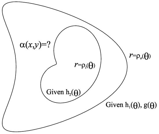
Figure 1. A schematic plot to show a doubly connected domain and for identification.

In the polar coordinates $(r,\theta )$, Equation (1) is recast to

$$\alpha \left[u_{rr}+\frac{1}{r}{u}_r+\frac{1}{r^2}{u}_{\theta \theta }\right]+{\alpha }_r{u}_r+\frac{1}{r^2}{\alpha }_{\theta }{u}_{\theta }=Q(u,u_r,u_{\theta })+S(r,\theta ).$$

(5)

Equation (5) is a first-order PDE for the function $\alpha (r,\theta )=\alpha (x,y)$ with respect to r and $\theta$, where $u_r$, $u_{\theta }$, $u_{rr}$ and $u_{\theta \theta }$ are the coefficient functions. It is a nontrivial task to determine $\alpha$ even with the known u prescribed inside the $\mathsf{\Omega }$ unless the boundary information of $\alpha$ on $\mathsf{\Gamma }$ is given in advance. Indeed, the inverse conductivity problem, which is considered in this paper, becomes more difficult and troublesome since the information of u is not given inside the solution domain, and only the boundary information is given according to Equations (2)–(4).

2.2. Temperature-Dependent Inverse Conductivity Problem

Secondly, we attempt to retrieve $\alpha \left(u\right)$ in

$$\left[u_{rr}+\frac{1}{r}{u}_r+\frac{1}{r^2}{u}_{\theta \theta }\right]\alpha \left(u\right)+{\alpha }^{\prime }\left(u\right)u_r^2+\frac{1}{r^2}{\alpha }^{\prime }\left(u\right)u_{\theta }^2=Q(u,u_r,u_{\theta })+S(r,\theta ),$$

(6)

when S and Q are given.

The temperature-dependent inverse conductivity problem is to determine the unknown conductivity function $\alpha \left(u\right)$ considering the above governing equation along with the information from Equations (2)–(4). The problem becomes harder for the reason that Equation (6) is nonlinear for u and linear ODE for $\alpha \left(u\right)$ with respect to u.

2.3. Inverse Robin Problem to Determine $\gamma \left(\theta \right)$

In the inner boundary, which is an inaccessible part of the boundary $\mathsf{\Gamma }$, we cannot directly detect the transfer coefficient $\gamma \left(\theta \right)$ in

$$u_n(x,y)+\gamma \left(\theta \right)u(x,y)=h_3(x,y),(x,y)\in {\mathsf{\Gamma }}_i.$$

(7)

When the information of $u(x,y)$ and $u_n(x,y)$ on ${\mathsf{\Gamma }}_i$ is unknown, $h_3(x,y)$ is given. Taken into the consideration of Equations (1)–(3), the unknown Robin coefficient $\gamma \left(\theta \right)$ will be recovered, which is known as the inverse Robin problem.

2.4. Inverse Problem for $S(x,y)$

When the function $u(x,y)$ is known in advance, we can recover $S(x,y)$ by

$$S(x,y)=\nabla ·[\alpha (x,y)\nabla u(x,y)]-Q(u,u_x,u_y),$$

(8)

where $\alpha (x,y)$ and $Q(u,u_x,u_y)$ are given functions. We will show that $S(x,y)$ is recoverable from Equations (2)–(4) and (8), without solving nonlinear equations.

3. Two-Parameter Basis Functions

First, we demonstrate the basic idea of homogenization function by starting from a 2D boundary value problem (BVP):

$$\begin{array}{ccc}\hfill & & \mathcal{L}\left[u\right(x,y\left)\right]=S(x,y),(x,y)\in (0,a)\times (0,b),\hfill \end{array}$$

(9)

$$\begin{array}{ccc}\hfill & & u(0,y)=h_1\left(y\right),u(a,y)=h_2\left(y\right),u(x,0)=h_3\left(x\right),u(x,b)=h_4\left(x\right),\hfill \end{array}$$

(10)

where $\mathcal{L}$ is a second-order linear differential operator. Let

$$B^0(x,y)=h_1\left(y\right)\left(1-\frac{x}{a}\right)+\frac{x}{a}{h}_2\left(y\right),$$

(11)

and then,

$$B^0(0,y)=h_1\left(y\right),B^0(a,y)=h_2\left(y\right)$$

(12)

are apparent.

Upon letting

$$B(x,y)=B^0(x,y)+\left(1-\frac{y}{b}\right)[h_3\left(x\right)-B^0(x,0)]+\frac{y}{b}[h_4\left(x\right)-B^0(x,b)],$$

(13)

and according to the following compatibility conditions:

$$\begin{array}{ccc}\hfill & & h_3\left(0\right)=B^0(0,0)=h_1\left(0\right),h_4\left(0\right)=B^0(0,b)=h_1\left(b\right),\hfill \\ & & h_3\left(a\right)=B^0(a,0)=h_2\left(0\right),h_4\left(a\right)=B^0(a,b)=h_2\left(b\right),\hfill \end{array}$$

(14)

it is easy to verify

$$B(0,y)=h_1\left(y\right),B(a,y)=h_2\left(y\right),B(x,0)=h_3\left(x\right),B(x,b)=h_4\left(x\right).$$

(15)

Therefore, we can produce the 2D homogenization function for the 2D BVP:

$$\begin{array}{ccc}\hfill & & B(x,y)=\left(1-\frac{x}{a}\right)\left[h_1\left(y\right)-\left(1-\frac{y}{b}\right)h_3\left(0\right)-\frac{y}{b}{h}_4\left(0\right)\right]\hfill \\ & & +\frac{x}{a}\left[h_2\left(y\right)-\left(1-\frac{y}{b}\right)h_3\left(a\right)-\frac{y}{b}{h}_4\left(a\right)\right]+\left(1-\frac{y}{b}\right)h_3\left(x\right)+\frac{y}{b}{h}_4\left(x\right).\hfill \end{array}$$

(16)

Due to $B(x,y)$, we can transform the original 2D BVP with non-homogeneous boundary conditions to one with homogeneous boundary conditions:

$$\begin{array}{ccc}\hfill & & \mathcal{L}\left[v\right(x,y\left)\right]=S(x,y)-\mathcal{L}\left[B\right(x,y\left)\right],(x,y)\in (0,a)\times (0,b),\hfill \end{array}$$

(17)

$$\begin{array}{ccc}\hfill & & v(0,y)=v(a,y)=v(x,0)=v(x,b)=0,\hfill \end{array}$$

(18)

with the help of the variable transformation from $u(x,y)$ to $v(x,y)=u(x,y)-B(x,y)$. Obviously, Equations (17) and (18) are more easy to tackle than Equations (9) and (10). As an extension of $B(x,y)$ to a two-parameter family, we have

$$\begin{array}{ccc}\hfill & & B(x,y,j,k)=\left[1-{\left(\frac{x}{a}\right)}^j\right]\left[h_1\left(y\right)-\left[1-{\left(\frac{y}{b}\right)}^k\right]h_3\left(0\right)-\frac{y}{b}{h}_4\left(0\right)\right]\hfill \\ & & +{\left(\frac{x}{a}\right)}^j\left[h_2\left(y\right)-\left(1-{\left(\frac{y}{b}\right)}^k\right)h_3\left(a\right)-{\left(\frac{y}{b}\right)}^k{h}_4\left(a\right)\right]+\left(1-{\left(\frac{y}{b}\right)}^k\right)h_3\left(x\right)+{\left(\frac{y}{b}\right)}^k{h}_4\left(x\right).\hfill \end{array}$$

(19)

$B(x,y,j,k)$ is indeed a family of 2D polynomials, which are complete bases and satisfy the boundary conditions automatically,

$$B(0,y,j,k)=h_1\left(y\right),B(a,y,j,k)=h_2\left(y\right),B(x,0,j,k)=h_3\left(x\right),B(x,b,j,k)=h_4\left(x\right).$$

(20)

A function is a so-called homogenization function if it satisfies the boundary conditions on the boundary of a domain. Since the solution $u(x,y)$ must satisfy the prescribed boundary conditions, it is a member of homogenization functions.

Continuously, the two-parameter homogenization functions are constructed for developing the present method to solve the inverse problems of Equations (1)–(4).

Definition 1.

$B^0(r,\theta )\in {\mathcal{C}}^2\left(\mathsf{\Omega }\right)$, with ${\mathsf{\Gamma }}_o=\left\{(r,\theta )\right|r={\rho }_o\left(\theta \right),0\le \theta \le 2\pi \}$, is a homogenization function, if the following conditions:

$$B^0({\rho }_o,\theta )=h_1\left(\theta \right),B_n^0({\rho }_o,\theta )=g\left(\theta \right)$$

(21)

are fulfilled. $h_1\left(\theta \right)$ and $g\left(\theta \right)$ read as $h_1({\rho }_o\left(\theta \right)cos\theta ,{\rho }_o\left(\theta \right)sin\theta )$ and $g({\rho }_o\left(\theta \right)cos\theta ,{\rho }_o\left(\theta \right)sin\theta )$, respectively, and $B_n^0$ signifying the normal derivative of $B^0(r,\theta )$ on ${\mathsf{\Gamma }}_o$ is given by

$$B_n^0({\rho }_o,\theta )=\eta \left(\theta \right)\left[\frac{\partial B^0({\rho }_o,\theta )}{\partial {\rho }_o}-\frac{{\rho }_o^{\prime }}{{\rho }_o^2}\frac{\partial B^0({\rho }_o,\theta )}{\partial \theta }\right],$$

(22)

where

$$\eta \left(\theta \right)=\frac{{\rho }_o\left(\theta \right)}{\sqrt{{\rho }_o^2\left(\theta \right)+{\rho }_o^{\prime }{\left(\theta \right)}^2}}.$$

(23)

The following homogenization function has been derived [18]:

$$\begin{array}{ccc}\hfill & & B^0(r,\theta )=h_1\left(\theta \right)+[r-{\rho }_o\left(\theta \right)]\frac{\partial u({\rho }_o,\theta )}{\partial {\rho }_o},\hfill \end{array}$$

(24)

$$\begin{array}{ccc}\hfill & & B^0({\rho }_o,\theta )=h_1\left(\theta \right),B_n^0({\rho }_o,\theta )=g\left(\theta \right).\hfill \end{array}$$

(25)

Theorem 1.

For the given Cauchy data $h_1\left(\theta \right)$ and $g\left(\theta \right)$ on ${\mathsf{\Gamma }}_o$, there exist homogenization functions $B(j,k,r,\theta )$ in Ω, satisfying Equation (21):

$$B(j,k,r,\theta )={\left[\frac{2r}{{\rho }_o}-\frac{r^2}{{\rho }_o^2}\right]}^j{h}_1\left(\theta \right)+\left[\frac{r^k}{k{\rho }_o^{k-1}}-\frac{{\rho }_o}{k}\right]\frac{\partial u({\rho }_o,\theta )}{\partial {\rho }_o},$$

(26)

where $j+1,k\in \mathbb{N}$ are parameters.

Proof. 

By Equation (26), $B(j,k,{\rho }_o,\theta )=h_1\left(\theta \right)$ satisfies the first equation in Equation (21). Next, we consider the second equation in Equation (21), for which we need to prove

$$\frac{\partial B(j,k,{\rho }_o,\theta )}{\partial {\rho }_o}=\frac{\partial u({\rho }_o,\theta )}{\partial {\rho }_o},\frac{\partial B(j,k,{\rho }_o,\theta )}{\partial \theta }=\frac{\partial u({\rho }_o,\theta )}{\partial \theta }.$$

(27)

It is obvious that

$$\begin{array}{ccc}\hfill & & {\left.{\left[\frac{2r}{{\rho }_o}-\frac{r^2}{{\rho }_o^2}\right]}^j\right|}_{r={\rho }_o}=1,{\left.\frac{\partial }{\partial r}{\left[\frac{2r}{{\rho }_o}-\frac{r^2}{{\rho }_o^2}\right]}^j\right|}_{r={\rho }_o}=0,\hfill \end{array}$$

(28)

$$\begin{array}{ccc}\hfill & & {\left.\frac{\partial }{\partial \theta }{\left[\frac{2r}{{\rho }_o}-\frac{r^2}{{\rho }_o^2}\right]}^j\right|}_{r={\rho }_o}={\left.j{\left[\frac{2r}{{\rho }_o}-\frac{r^2}{{\rho }_o^2}\right]}^{j-1}\left[\frac{-2r{\rho }_o^{\prime }}{{\rho }_o^2}+\frac{2r^2{\rho }_o^{\prime }}{{\rho }_o^3}\right]\right|}_{r={\rho }_o}=0,\hfill \end{array}$$

(29)

$$\begin{array}{ccc}\hfill & & {\left.\left[\frac{r^k}{k{\rho }_o^{k-1}}-\frac{{\rho }_o}{k}\right]\right|}_{r={\rho }_o}=0,{\left.\frac{\partial }{\partial r}\left[\frac{r^k}{k{\rho }_o^{k-1}}-\frac{{\rho }_o}{k}\right]\right|}_{r={\rho }_o}=1,\hfill \end{array}$$

(30)

$$\begin{array}{ccc}\hfill & & {\left.\frac{\partial }{\partial \theta }\left[\frac{r^k}{k{\rho }_o^{k-1}}-\frac{{\rho }_o}{k}\right]\right|}_{r={\rho }_o}={\left.\left[\frac{r^k}{k}(1-k){\rho }_o^{-k}{\rho }_o^{\prime }-\frac{{\rho }_o^{\prime }}{k}\right]\right|}_{r={\rho }_o}=-{\rho }_o^{\prime }.\hfill \end{array}$$

(31)

It follows from Equations (26), (28) and (30) that the first part in Equation (27) holds when $B(j,k,r,\theta )$ is differentiated to r, and we take $r={\rho }_o\left(\theta \right)$ on ${\mathsf{\Gamma }}_o$.

The second part in Equation (27) is proven below. It follows from Equation (2) that

$$h_1^{\prime }\left(\theta \right)=\frac{\partial u({\rho }_o,\theta )}{\partial {\rho }_o}{\rho }_o^{\prime }\left(\theta \right)+\frac{\partial u({\rho }_o,\theta )}{\partial \theta }.$$

(32)

From Equations (26) and (28)–(32), it follows that

$$\begin{array}{ccc}\hfill & & \frac{\partial B(j,k,{\rho }_o,\theta )}{\partial \theta }=h_1^{\prime }\left(\theta \right)-{\rho }_o^{\prime }\left(\theta \right)\frac{\partial u({\rho }_o,\theta )}{\partial {\rho }_o}\hfill \\ & & =\frac{\partial u({\rho }_o,\theta )}{\partial {\rho }_o}{\rho }_o^{\prime }\left(\theta \right)+\frac{\partial u({\rho }_o,\theta )}{\partial \theta }-{\rho }_o^{\prime }\left(\theta \right)\frac{\partial u({\rho }_o,\theta )}{\partial {\rho }_o}=\frac{\partial u({\rho }_o,\theta )}{\partial \theta }.\hfill \end{array}$$

(33)

Due to Equation (27),

$$\begin{array}{ccc}\hfill & & B_n(j,k,{\rho }_o,\theta )=\eta \left(\theta \right)\left[\frac{\partial B(j,k,{\rho }_o,\theta )}{\partial {\rho }_o}-\frac{{\rho }_o^{\prime }}{{\rho }_o^2}\frac{\partial B(j,k,{\rho }_o,\theta )}{\partial \theta }\right]\hfill \\ & & =\eta \left(\theta \right)\left[\frac{\partial u({\rho }_o,\theta )({\rho }_o,\theta )}{\partial {\rho }_o}-\frac{{\rho }_o^{\prime }}{{\rho }_o^2}\frac{\partial u({\rho }_o,\theta )}{\partial \theta }\right]=g\left(\theta \right)=u_n(x,y),(x,y)\in {\mathsf{\Gamma }}_o,\hfill \end{array}$$

(34)

thus we prove

$$B(j,k,{\rho }_o,\theta )=h_1\left(\theta \right),B_n(j,k,{\rho }_o,\theta )=g\left(\theta \right),$$

(35)

which ends the proof of this theorem. □

In Theorem 1, the numbers $(j,k)$ are parameters, and then $B(j,k,r,\theta )$ is a two-parameter function. In addition to Theorem 1, we also have the following result for another two-parameter function $E(j,k,r,\theta )$.

Theorem 2.

On ${\mathsf{\Gamma }}_o$ given the Cauchy data $h_1\left(\theta \right)$ and $g\left(\theta \right)$, the two-parameter function $E(j,k,r,\theta )\in {\mathcal{C}}^2\left(\mathsf{\Omega }\right)$ satisfies Equation (21):

$$E(j,k,r,\theta )=B^0(r,\theta )+{[r-{\rho }_o\left(\theta \right)]}^2{x}^{j-k}{y}^k=B^0(r,\theta )+{[r-{\rho }_o\left(\theta \right)]}^2{r}^j{(cos\theta )}^{j-k}{(sin\theta )}^k,$$

(36)

where $j+1,k\in \mathbb{N}$ are parameters and $B^0$ was defined by Equation (24).

Proof. 

Let

$$E^0(r,\theta ):={[r-{\rho }_o\left(\theta \right)]}^2.$$

When $r={\rho }_o\left(\theta \right)$, it is obvious that

$$E^0(r,\theta )={[r-{\rho }_o\left(\theta \right)]}^2=0,E_n^0(r,\theta )=2[r-{\rho }_o\left(\theta \right)]{[r-{\rho }_o\left(\theta \right)]}_n=0.$$

(37)

Inserting $r={\rho }_o\left(\theta \right)$ into Equation (36) and using Equations (24), (25) and (37), it follows that

$$E(j,k,{\rho }_o,\theta )=h_1\left(\theta \right).$$

Taking the normal derivative of Equation (36) on ${\mathsf{\Gamma }}_o$ and using Equations (24), (25) and (37), we have

$$\begin{array}{ccc}& & E_n(j,k,\rho ,\theta )=B_n^0({\rho }_o,\theta )+E_n^0(r,\theta )r^j{(cos\theta )}^{j-k}{(sin\theta )}^k+E^0(r,\theta ){\left[r^j{(cos\theta )}^{j-k}{(sin\theta )}^k\right]}_n\hfill \\ & & =B_n^0({\rho }_o,\theta )=g\left(\theta \right),whenr={\rho }_o\left(\theta \right).\hfill \end{array}$$

This completes the proof. □

4. A Novel Two-Parameter Homogenization Function Method

Since the set $E(j,k,r,\theta )$ is generated from the Pascal polynomials $x^{j-k}{y}^k$, it is a complete basis for the problem. By the same token, $B(j,k,r,\theta )$ is a complete basis. All the homogenization functions consist of a weighted Sobolev space denoted as $\mathcal{B}:=\{v(x,y)\in {\mathcal{C}}^2\left(\mathsf{\Omega }\right)|v(x,y)=h_1(x,y),v_n(x,y)=g(x,y),(x,y)\in {\mathsf{\Gamma }}_o\}$, which is a weighted space, because for any two functions $v_1(x,y),v_2(x,y)\in \mathcal{B}$ with a weighted linear combination $w_1{v}_1(x,y)+w_2{v}_2(x,y)\in \mathcal{B}$ where $w_1+w_2=1$. The Sobolev norm

$${\parallel v(x,y)\parallel }^2:={\int }_0^{2\pi }[v^2({\rho }_{o}cos\theta ,{\rho }_{o}sin\theta )+v_n^2({\rho }_{o}cos\theta ,{\rho }_{o}sin\theta )]d\theta$$

(38)

is defined in the space $\mathcal{B}$. More importantly, the approximate solution $u(x,y)\in \mathcal{B}$.

In terms of the bases $B(j,k,x,y)$, $u(x,y)$ can be expanded by

$$u(x,y)\approx \sum _{j=0}^{m-1}\sum _{k=1}^m{a}_{jk}B(j,k,x,y),$$

(39)

where $a_{jk}$ satisfies

$$\sum _{j=0}^{m-1}\sum _{k=1}^m{a}_{jk}=1,$$

(40)

and guarantees conditions (2) and (3) being satisfied by $u(x,y)$. The number of the coefficients $a_{jk}$ is $n_1=m^2$.

As shown in Equation (4), we suppose that there are N data of $u(x,y)$ on the inner boundary ${\mathsf{\Gamma }}_i$ available, and then we can solve a linear system, including Equation (40), to determine $a_{jk}$:

$$\sum _{j=0}^{m-1}\sum _{k=1}^m{a}_{jk}B(j,k,x_q,y_q)=h_2(x_q,y_q),$$

(41)

where ${\theta }_q=2q\pi /N$, $x_q={\rho }_i\left({\theta }_q\right)cos{\theta }_q$ and $y_q={\rho }_i\left({\theta }_q\right)sin{\theta }_q$.

5. Numerical Procedure to Determine $\mathit{\alpha }(\mathit{x},\mathit{y})$

5.1. Numerical Algorithm

Next, when $u(x,y)$ is obtained from Equation (39), we recover $\alpha (x,y)$ by supposing

$$\alpha (x,y)=\sum _{i=0}^{m_0}\sum _{j=0}^i{b}_{ij}{x}^{i-j}{y}^j=\sum _{i=0}^{m_0}\sum _{j=0}^i{b}_{ij}{r}^i{(cos\theta )}^{i-j}{(sin\theta )}^j,$$

(42)

where $b_{ij}$ are $n:=(m_0+1)(m_0+2)/2$ unknown weighted parameters to be determined by the proposed numerical algorithm. In order to solve this problem, $m_1\times m_2$ points of $(x,y)$ inside the solution domain $\mathsf{\Omega }$ are collocated by

$$\begin{array}{ccc}\hfill & & x_{pq}=r_{p}cos{\theta }_q,y_{pq}=r_{p}sin{\theta }_q,\hfill \\ & & {\theta }_q=2q\pi /m_1,r_p={\rho }_i\left({\theta }_q\right)+p[{\rho }_o\left({\theta }_q\right)-{\rho }_i\left({\theta }_q\right)]/(m_2+1),q=1,\dots ,m_1,p=1,\dots ,m_2.\hfill \end{array}$$

(43)

Since $u(x,y)$ can be approximated by Equation (39), we have

$$u(x_{pq},y_{pq})=\sum _{j=0}^{m-1}\sum _{k=1}^m{a}_{jk}B(j,k,x_{pq},y_{pq}).$$

(44)

Then, inserting Equation (42) into Equation (5) and collocating at point $(x_{pq},y_{pq})$, the following linear system can be obtained:

$$\begin{array}{ccc}\hfill & & \Delta u(x_{pq},y_{pq})\sum _{i=0}^{m_0}\sum _{j=0}^i{b}_{ij}{x}_{pq}^{i-j}{y}_{pq}^j+u_r(x_{pq},y_{pq})\sum _{i=0}^{m_0}\sum _{j=0}^{i}i{b}_{ij}{r}_p^{i-1}{(cos{\theta }_q)}^{i-j}{(sin{\theta }_q)}^j\hfill \\ & & +\frac{1}{r_p^2}{u}_{\theta }(x_{pq},y_{pq})\sum _{i=0}^{m_0}\sum _{j=0}^i{b}_{ij}{r}_p^i[j{(cos{\theta }_q)}^{i-j+1}{(sin{\theta }_q)}^{j-1}-(i-j){(cos{\theta }_q)}^{i-j-1}{(sin{\theta }_q)}^{j+1}]\hfill \\ & & =Q(u(x_{pq},y_{pq}),u_r(x_{pq},y_{pq}),u_{\theta }(x_{pq},y_{pq}))+S(r_p,{\theta }_q),q=1,\dots ,m_1,p=1,\dots ,m_2,\hfill \end{array}$$

(45)

from which we can determine $b_{ij}$ easily, and, correspondingly, the $\alpha (x,y)$ can be determined from Equation (42).

Therefore, the proposed algorithm for recovering $\alpha (x,y)$ consists of two linear systems of equations, Equations (41) and (45). We impose the data by a noise:

$${\widehat{h}}_1\left({\theta }_j\right)=h_1\left({\theta }_j\right)+sR\left(j\right),\widehat{g}\left({\theta }_j\right)=g\left({\theta }_j\right)+sR\left(j\right),$$

(46)

where $R\left(j\right)$ are random numbers between $[-1,1]$, which are used to check the stability of the numerical solution.

To evaluate the accuracy, we consider the maximum error (ME) and a relative error defined by

$$\begin{array}{ccc}\hfill & & \mathrm{ME}\left(\alpha \right):=max|{\alpha }_n(x_{pq},y_{pq})-\alpha (x_{pq},y_{pq})|,\hfill \end{array}$$

(47)

$$\begin{array}{ccc}\hfill & & e\left(\alpha \right)=\sqrt{\frac{{\sum }_{q=1}^{N_1}{\sum }_{p=1}^{N_2}{[{\alpha }_n(x_{pq},y_{pq})-\alpha (x_{pq},y_{pq})]}^2}{{\sum }_{q=1}^{N_1}{\sum }_{p=1}^{N_2}{\alpha }^2(x_{pq},y_{pq})}},\hfill \end{array}$$

(48)

upon comparing the numerical solution of ${\alpha }_n$ to the exact one $\alpha$ at $N_1\times N_2$ grid points $(x_i,y_j)$ inside the domain with

$$\begin{array}{ccc}\hfill & & x_{pq}=r_{p}cos{\theta }_q,y_{pq}=r_{p}sin{\theta }_q,\hfill \\ & & {\theta }_q=2q\pi /N_1,r_p={\rho }_i\left({\theta }_q\right)+p[{\rho }_o\left({\theta }_q\right)-{\rho }_i\left({\theta }_q\right)]/(N_2+1),q=1,\dots ,N_1,p=1,\dots ,N_2.\hfill \end{array}$$

(49)

We take $N_1=50$ and $N_2=10$ in all computations.

We must emphasize that all the linear systems we consider are over-determined, which means that the number of linear equations is much larger than the number of unknown coefficients. Therefore, we apply the conjugate gradient method (CGM) to solve the corresponding normal linear system, whose solution is unique in the sense of least squares.

5.2. Example 1

For Equation (5) with $Q=0$, we consider

$$u=r^2+rcos\theta =x^2+y^2+x,\alpha =10+r^2+r^4{cos}^2\theta =10+(x^2+y^2)(x^2+1).$$

(50)

The outer boundary of the domain $\mathsf{\Omega }$ is an ellipse:

$${\rho }_o\left(\theta \right)=\frac{ab}{\sqrt{b^2+(a^2-b^2){sin}^2\theta }},$$

(51)

where we take $a=1.5$ and $b=0.5$, and the inner boundary is ${\rho }_i=0.2$.

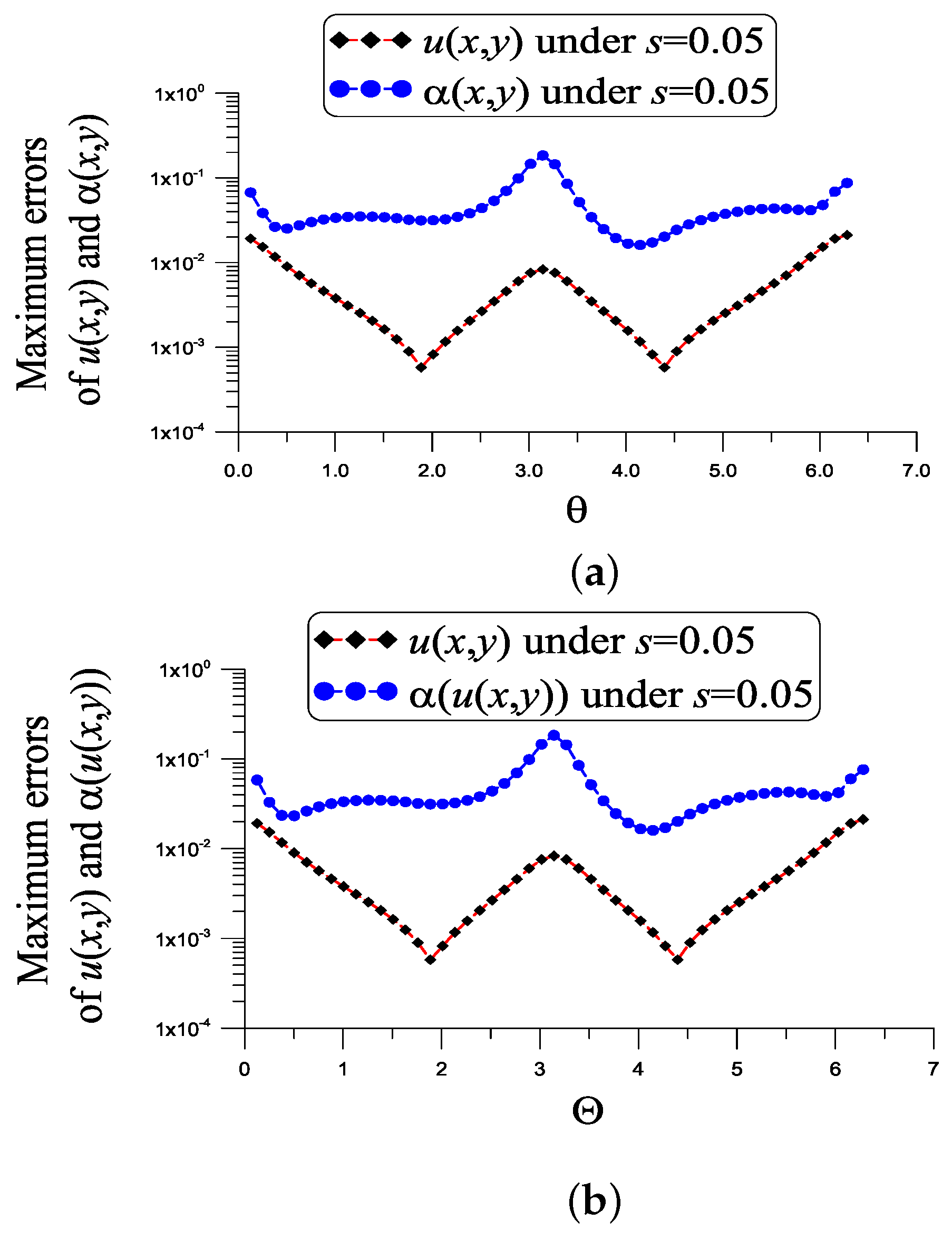
With $m=2$, $N=40$, $m_0=4$, $m_1=30$, $m_2=10$ and a noise $s=5\%$ added into the given data, Figure 2a reveals that the maximum absolute error of u is $2.11\times {10}^{-2}$, which is much smaller than $max\left(u\right)=3.29$. The maximum absolute error of coefficient $\alpha (x,y)$ denoted as ME$\left(\alpha \right)$ is 0.18, which is quite a lot smaller than $max\left(\alpha \right)=15.56$. The value $e\left(\alpha \right)=3.8\times {10}^{-3}$ is smaller than $7.65\times {10}^{-2}$ from previous studies. For this problem the dimension of the normal matrix of the first linear system of (41) and (40) is $n_1\times n_1=4\times 4$, and the condition number is small with COND = 570.046. The dimension of the normal matrix of the second linear system (45) is $n\times n=15\times 15$, and the condition number is COND = 41,996.23. They show that these two linear systems are stable.

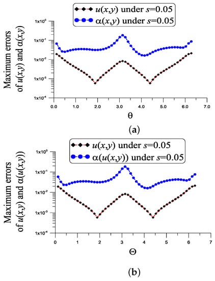
Figure 2. For example 1, showing the errors in the numerical recovery of u and $\alpha$ under a noise $s=0.05$, (a) $Q=0$ and (b) $Q=u^2$.

The convergence rate is a central issue in numerical methods and algorithms. In Table 1, we consider a different mesh parameter $m_1\times m_2$ used in the collocation method to influence the convergence rate as reflected in ME($\alpha$) and $e\left(\alpha \right)$. It can be seen that more collocated points lead to a more accurate solution of $\alpha$.

Table 1. For example 1, the influence of mesh parameter $m_1\times m_2$ on ME($\alpha$) and $e\left(\alpha \right)$.

${\mathit{m}}_1\times {\mathit{m}}_2$	$5\times 5$	$7\times 5$	$10\times 10$	$10\times 5$	$30\times 10$
ME($\alpha$)	7.7369	1.8430	0.4017	0.2147	0.18364
$e\left(\alpha \right)$	$1.46\times {10}^{-1}$	$2.34\times {10}^{-2}$	$1.83\times {10}^{-2}$	$5.15\times {10}^{-2}$	$3.79\times {10}^{-3}$

Although for a nonlinear elliptic equation:

$$\alpha \left[u_{rr}+\frac{1}{r}{u}_r+\frac{1}{r^2}{u}_{\theta \theta }\right]+{\alpha }_r{u}_r+\frac{1}{r^2}{\alpha }_{\theta }{u}_{\theta }=u^2(r,\theta )+S(r,\theta ),$$

(52)

where the exact value of $S(r,\theta )$ can be obtained by inserting Equation (50) into the above equation, as shown in Figure 2b, the ME of u is $2.11\times {10}^{-2}$, the ME of $\alpha (x,y)$ is 0.18 and $e\left(\alpha \right)=3.74\times {10}^{-3}$. For the nonlinear problem, we have the same condition numbers because the parameters used are the same.

5.3. Example 2

Consider

$$\begin{array}{ccc}\hfill & & \alpha \left[u_{rr}+\frac{1}{r}{u}_r+\frac{1}{r^2}{u}_{\theta \theta }\right]+{\alpha }_r{u}_r+\frac{1}{r^2}{\alpha }_{\theta }{u}_{\theta }=sinu(r,\theta )+u^2(r,\theta )+S(r,\theta ),\hfill \end{array}$$

(53)

$$\begin{array}{ccc}\hfill & & u=r^2+rcos\theta =x^2+y^2+x,\alpha =20+r^{2}sin\left(2\theta \right)=20+2xy.\hfill \end{array}$$

(54)

For this problem, the outer boundary is given by Equation (51) with $a=4$ and $b=3.5$, and

$${\rho }_i\left(\theta \right)=1.5+cos\theta$$

(55)

is the inner boundary. Feeding Equation (54) into Equation (53), $S(r,\theta )$ can be obtained.

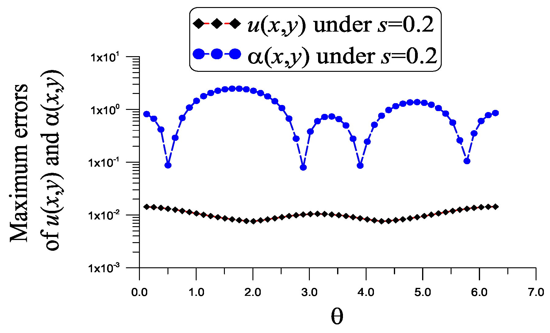
With $m=2$, $N=50$, $m_0=2$, $m_1=10$, $m_2=10$ and a noise $s=20\%$, as shown in Figure 3, the ME of u is $1.44\times {10}^{-2}$, which is much smaller than $max\left(u\right)=18.79$. The ME of $\alpha (x,y)$ is 2.47, which is much smaller than $max\left(\alpha \right)=32.96$. The value $e\left(\alpha \right)=3.85\times {10}^{-2}$ is small. For this problem the dimension of the normal matrix of the first linear system (41) and (40) is $n_1\times n_1=4\times 4$, and the condition number is small with COND = 1844.258. The dimension of the normal matrix of the second linear system (45) is $n\times n=6\times 6$, and the condition number is COND = 1013.03. They show that these two linear systems are stable.

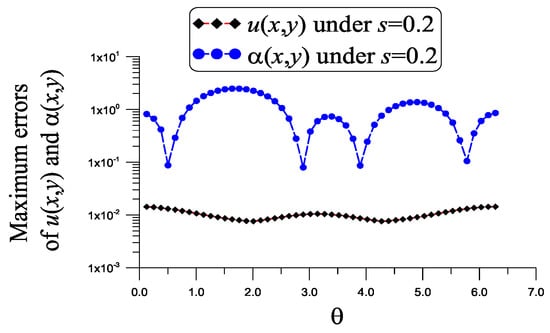
Figure 3. For example 2, showing the errors in the numerical recovery of u and $\alpha$ under a noise $s=0.2$ with $Q=u^2+sinu$.

6. Numerical Algorithm to Determine $\mathit{\alpha }\left(\mathit{u}\right)$

6.1. Numerical Algorithm

From the last section, we have already recovered the coefficients preceding $\alpha \left(u\right)$ and $u_r^2+u_{\theta }^2/r^2$ preceding ${\alpha }^{\prime }\left(u\right)$ in Equation (6), if Q and S are prescribed in advance. Indeed $u(x,y)$ can be derived from Equation (39). In this case, $\Delta u$ before $\alpha \left(u\right)$, and $u_r^2+u_{\theta }^2/r^2$ before ${\alpha }^{\prime }\left(u\right)$ can be obtained numerically from Equation (39).

Suppose that

$$\alpha \left(u\right)=\sum _{i=0}^{m_0}{c}_i{u}^i,$$

(56)

where $c_i$ are under-determined weighted parameters to be determined.

Similar to Equation (43) in the last section, we arrange $m_1\times m_2$ points of $(x,y)$ inside the solution domain. Then, inserting Equation (56) into Equation (6) and collocating $(x_{pq},y_{pq})$, we come to

$$\begin{array}{ccc}\hfill & & \sum _{i=0}^{m_0}{c}_i{u}^i(x_{pq},y_{pq})\Delta u(x_{pq},y_{pq})+\sum _{i=0}^{m_0}{c}_{i}i{u}^{i-1}(x_{pq},y_{pq})[u_r^2(x_{pq},y_{pq})+u_{\theta }^2(x_{pq},y_{pq})/r_p^2]\hfill \\ & & =Q(u(x_{pq},y_{pq}),u_r(x_{pq},y_{pq}),u_{\theta }(x_{pq},y_{pq}))+S(x_{pq},y_{pq}),p=1,\dots ,m_2,q=1,\dots ,m_1.\hfill \end{array}$$

(57)

from which we can obtain $c_i$, and then, $\alpha \left(u\right)$ is recovered from Equation (56).

It should be noted here that that even for the highly nonlinear inverse problems for coefficient $\alpha \left(u\right)$, solving nonlinear equations is not needed.

6.2. Example 3

For a quadratic nonlinear Poisson equation:

$$\begin{array}{ccc}\hfill & & \Delta u\alpha \left(u\right)+{\alpha }^{\prime }\left(u\right)u_r^2+\frac{1}{r^2}{\alpha }^{\prime }\left(u\right)u_{\theta }^2+u^2=S(r,\theta ),\hfill \end{array}$$

(58)

$$\begin{array}{ccc}& & u=r^2=x^2+y^2,\hfill \end{array}$$

(59)

$\alpha \left(u\right)=10+u^2+u$ is to be recovered. The outer boundary is Equation (51) with $a=3.5$ and $b=2.5$, and ${\rho }_i=1$ is a unit circle.

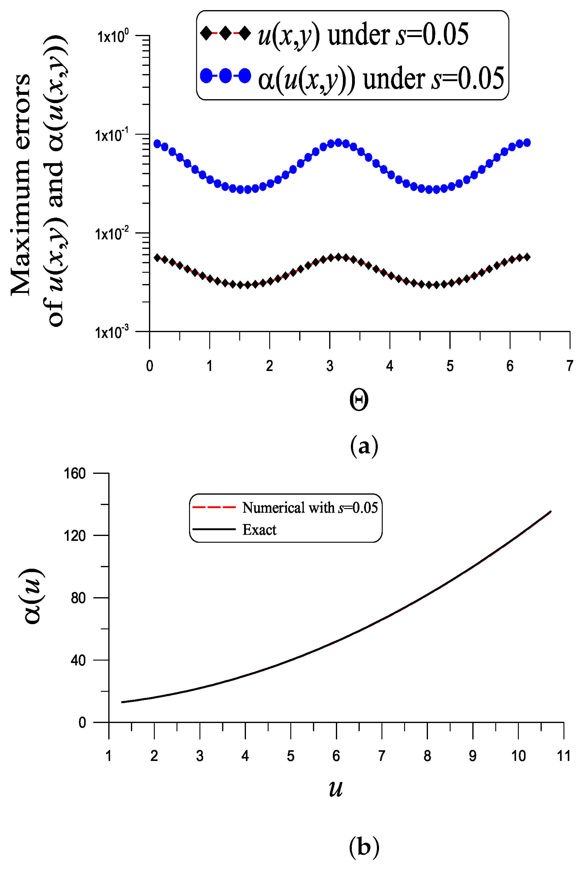
With $m=2$, $N=40$, $m_0=2$, $m_1=20$, $m_2=5$ and $s=5\%$, as shown in Figure 4a, the ME of u is $5.68\times {10}^{-3}$, which is much smaller than $max\left(u\right)=10.7$. The ME of $\alpha \left(u\right)$ is 0.082, which is much smaller than $max\left(\alpha \right)=135.43$. The value $e\left(\alpha \right)=6.03\times {10}^{-4}$ is quite small. Figure 4b compares the numerical and exact $\alpha \left(u\right)$ in the range of $u\le 11$. These two curves almost coincide.

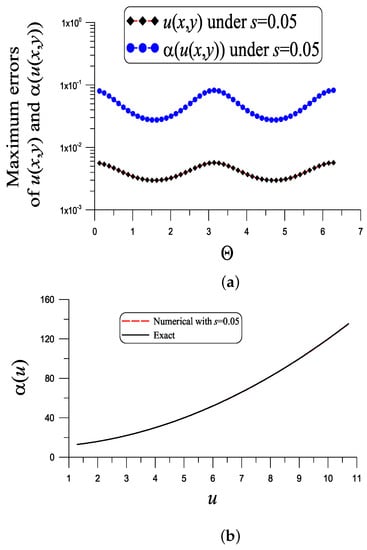
Figure 4. For example 3, showing (a) the errors in the numerical recovery of u and $\alpha$ and (b) the numerical recovery of $\alpha$ under a noise $s=0.05$.

For this problem, the dimension of the normal matrix of the first linear system (41) and (40) is $n_1\times n_1=4\times 4$, and the condition number is very small with COND = 33.959. The dimension of the normal matrix of the second linear system (57) is $n\times n=3\times 3$, and the condition number is COND = 177,571.79. They show that these two linear systems are stable.

6.3. Example 4

For a quadratic and cubic nonlinear Poisson equation:

$$\begin{array}{ccc}\hfill & & \Delta u\alpha \left(u\right)+{\alpha }^{\prime }\left(u\right)u_r^2+\frac{1}{r^2}{\alpha }^{\prime }\left(u\right)u_{\theta }^2+u^2+u^3=S(r,\theta ),\hfill \end{array}$$

(60)

$$\begin{array}{ccc}& & u=r^2=x^2+y^2,\hfill \end{array}$$

(61)

$\alpha \left(u\right)=10+u^2+sinu$ is to be recovered. The boundaries of $\mathsf{\Omega }$ are given by

$$\begin{array}{ccc}\hfill & & {\rho }_o\left(\theta \right)=3\sqrt{cos\left(2\theta \right)+\sqrt{1.5-{sin}^2\left(2\theta \right)}},\hfill \end{array}$$

(62)

$$\begin{array}{ccc}\hfill & & {\rho }_i\left(\theta \right)=exp(sin\theta ){sin}^2\left(2\theta \right)+exp(cos\theta ){cos}^2\left(2\theta \right).\hfill \end{array}$$

(63)

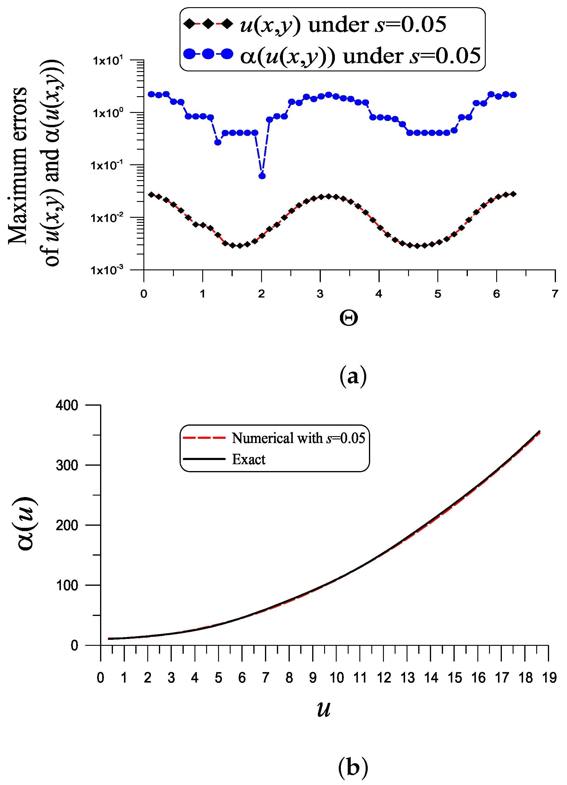
With $m=2$, $N=40$, $m_0=3$, $m_1=15$, $m_2=10$ and $s=5\%$, as shown in Figure 5a, the ME of u is $2.78\times {10}^{-2}$, which is much smaller than $max\left(u\right)=18.6$. The ME of $\alpha \left(u\right)$ is 2.23, which is much smaller than $max\left(\alpha \right)=356.45$. The value $e\left(\alpha \right)=9.35\times {10}^{-3}$ is quite small. Figure 5b compares the numerical and exact $\alpha \left(u\right)$ in the range of $u\le 19$. These two curves almost coincide.

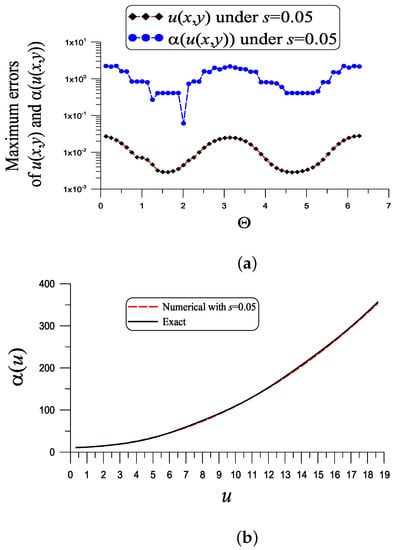
Figure 5. For example 4, showing (a) the errors in the numerical recovery of u and $\alpha$ and (b) the numerical recovery of $\alpha$ under a noise $s=0.05$.

For this problem, the dimension of the normal matrix of the first linear system (41) and (40) is $n_1\times n_1=4\times 4$, and the condition number is very small with COND = 6.3185. The dimension of the normal matrix of the second linear system (57) is $n\times n=4\times 4$, and the condition number is COND = $2.15\times {10}^8$.

To reduce the condition number for the second linear system (57), we choose $m_0=2$, $m_1=10$ and $m_2=10$, such that the dimension of the normal matrix reduces to $n\times n=3\times 3$, and the condition number reduces to COND = 297,651.317. Meanwhile, ME$\left(\alpha \right)$ and $e\left(\alpha \right)$ are slightly increased to 2.38 and $1.08\times {10}^{-2}$, respectively.

7. Numerical Method to Detect $\mathbf{\gamma }\left(\mathbf{\theta }\right)$

7.1. Numerical Method

Now, we detect $\gamma \left(\theta \right)$ by using the data in Equations (2) and (3). Basically, we need to solve Equations (1)–(3) in $\mathsf{\Omega }$. For this purpose, we take

$$u(x,y)=\sum _{j=0}^m\sum _{k=0}^j{a}_{jk}E(j,k,x,y),$$

(64)

where the number of $a_{jk},j,k=1,\dots ,m$ is $n_1=(m+1)(m+2)/2$, which are to be determined. Instead of $B(j,k,x,y)$ used in Equation (39), we employ $E(j,k,x,y)$ from Equation (36) as the bases of $u(x,y)$. The reason is that the order of $r^{j+2}$ in $E(j,k,x,y)$ is much lower than the order of $r^{2j}$ in $B(j,k,x,y)$.

Like Equation (43), we arrange $m_1\times m_2$ points of $(x,y)$ and collocating which comes to:

$$\begin{array}{ccc}\hfill & & \alpha (x_{pq},y_{pq})\sum _{j=0}^m\sum _{k=0}^j{a}_{jk}\Delta E(j,k,x_{pq},y_{pq})+{\alpha }_x(x_{pq},y_{pq})\sum _{j=0}^m\sum _{k=0}^j{a}_{jk}{E}_x(j,k,x_{pq},y_{pq})\hfill \\ & & +{\alpha }_y(x_{pq},y_{pq})\sum _{j=0}^m\sum _{k=0}^j{a}_{jk}{E}_y(j,k,x_{pq},y_{pq})\hfill \\ & & =Q\left(\sum _{j=0}^m\sum _{k=0}^j{a}_{jk}E(j,k,x_{pq},y_{pq}),\sum _{j=0}^m\sum _{k=0}^j{a}_{jk}{E}_x(j,k,x_{pq},y_{pq}),\sum _{j=0}^m\sum _{k=0}^j{a}_{jk}{E}_y(j,k,x_{pq},y_{pq})\right)\hfill \\ & & +S(x_{pq},y_{pq}),p=1,\dots ,m_2,q=1,\dots ,m_1.\hfill \end{array}$$

(65)

from which we can compute $a_{jk}$, and then $u(x,y)$ is obtained from Equation (64), which is inserted in Equation (7) to find $\gamma \left(\theta \right)$ along the inner boundary ${\mathsf{\Gamma }}_i$.

7.2. Example 5

We give a solution of a linear diffusion-convection equation:

$$\begin{array}{ccc}\hfill & & \alpha \Delta u(x,y)+{\alpha }_x{u}_x(x,y)+{\alpha }_y{u}_y(x,y)=S(x,y),\hfill \end{array}$$

(66)

$$\begin{array}{ccc}& & u=x^2+y^2+x,\hfill \end{array}$$

(67)

where $\alpha =1+x^2+y^2$, which is defined in a domain $\mathsf{\Omega }$ by Equation (51) with $a=2.5$ and $b=1.5$ and by

$${\rho }_i\left(\theta \right)=1.3+0.1cos\theta .$$

(68)

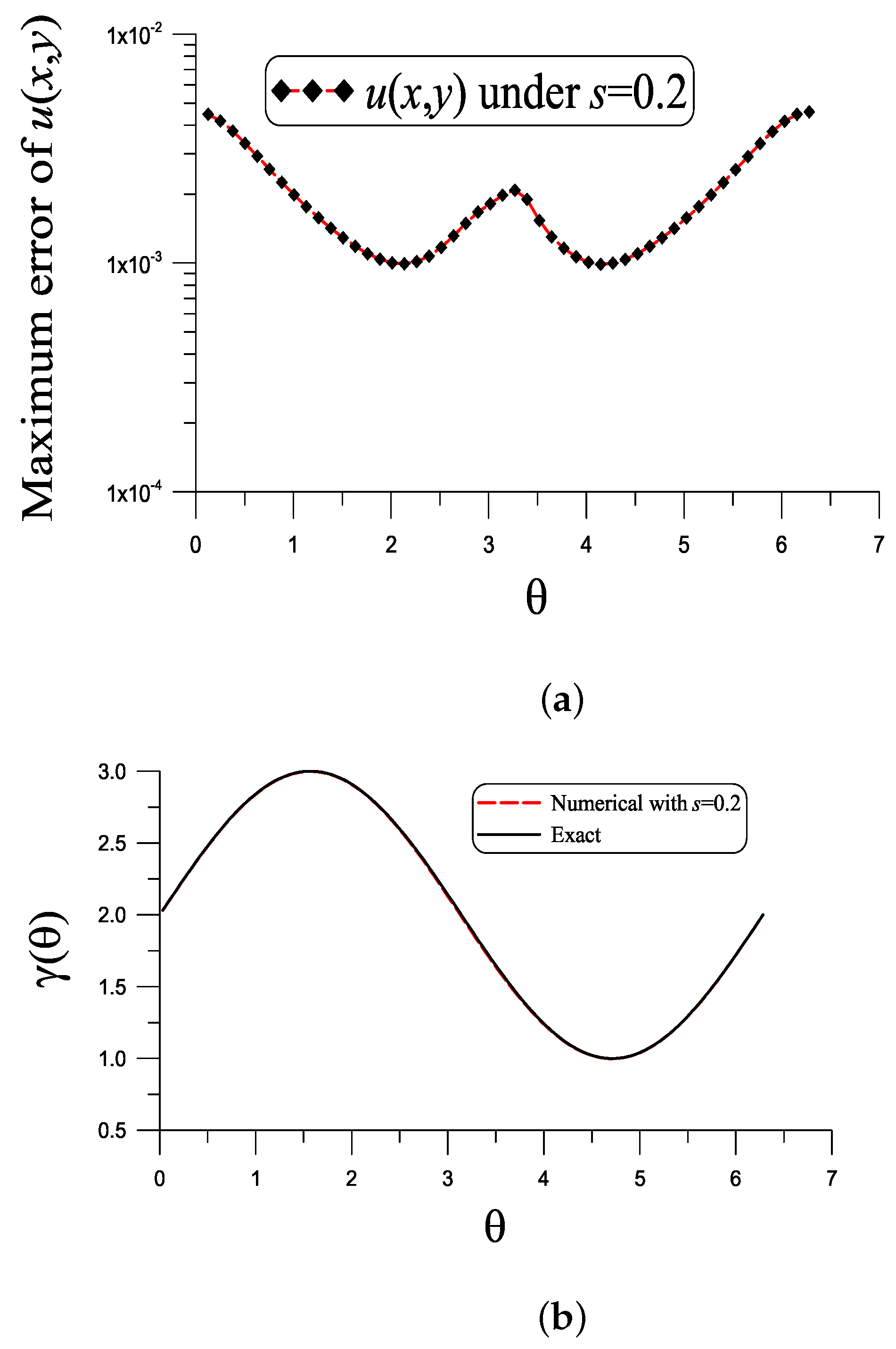
With $m=2$, $m_1=20$, $m_2=20$ and $s=20\%$, as shown in Figure 6a, the ME of u is $4.58\times {10}^{-3}$, which is much smaller than $max\left(u\right)=8.16$. Figure 6b compares the numerical and exact $\gamma \left(\theta \right)$, of which these two curves almost coincide with the ME being $1.28\times {10}^{-2}$. For this problem, we merely solve the linear system (65) and (40), whose dimension of the normal matrix is $n_1\times n_1=6\times 6$, and the condition number is small with COND = 446.16.

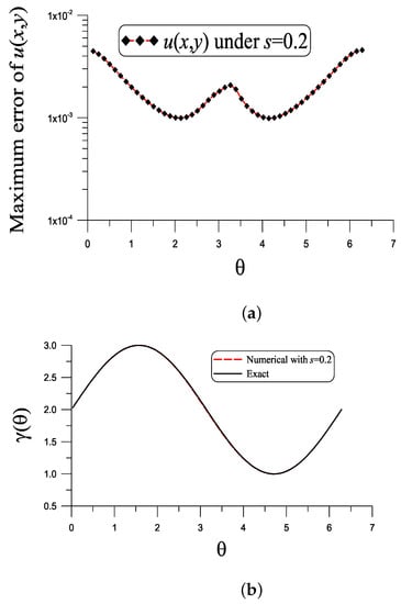
Figure 6. For example 5, showing (a) the error in the numerical recovery of u and (b) comparing the numerical recovery of $\gamma$ under a noise $s=0.2$.

8. Numerical Method to Recover $\mathit{S}(\mathit{x},\mathit{y})$

The numerical method to recover $S(x,y)$ is very simple, which is obtained by merely inserting the numerical solution of $u(r,\theta )$ in Equation (39) into the following equation:

$$S(r,\theta )=\alpha \left[u_{rr}+\frac{1}{r}{u}_r+\frac{1}{r^2}{u}_{\theta \theta }\right]+{\alpha }_r{u}_r+\frac{1}{r^2}{\alpha }_{\theta }{u}_{\theta }-Q(u(r,\theta ),u_r(r,\theta ),u_{\theta }(r,\theta )),$$

(69)

where $\alpha (r,\theta )$ and $Q(u(r,\theta ),u_r(r,\theta ),u_{\theta }(r,\theta ))$ are given functions.

8.1. Example 6

For Equation (69) with $Q=u^2$, we consider

$$u=r^2+rcos\theta =x^2+y^2+x,\alpha =10+r^2+r^4{cos}^2\theta =10+(x^2+y^2)(x^2+1),$$

(70)

with $a=1.5$ and $b=0.5$ in Equation (51), and we take ${\rho }_i=0.2$.

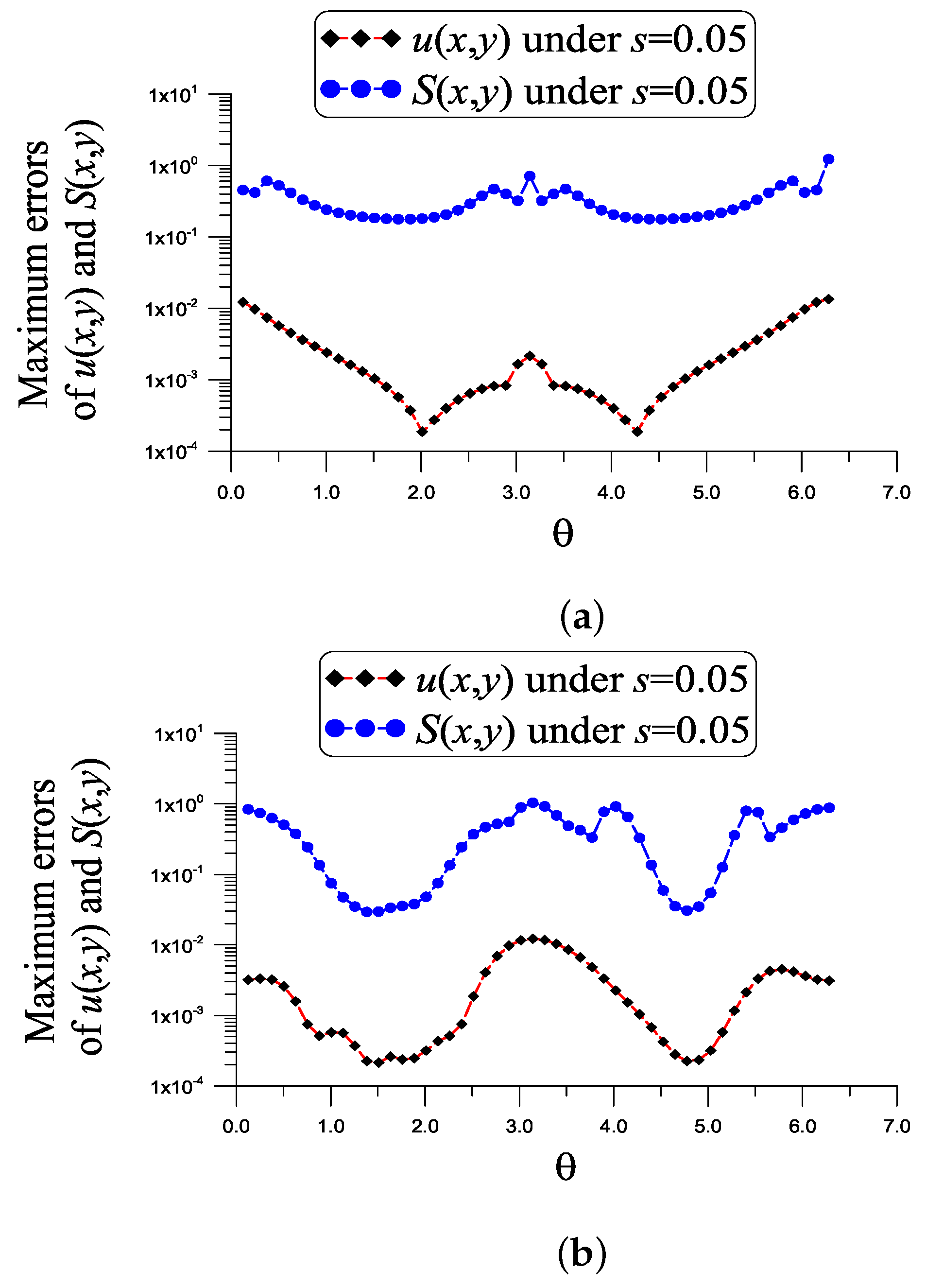
In this case, we have $m=2$, $N=30$ and a noise $s=5\%$ added into the given data, as shown in Figure 7a, the maximum absolute error of u is $1.35\times {10}^{-2}$, which is much smaller than $max\left(u\right)=3.29$. The maximum absolute error of $S(x,y)$, denoted as ME$\left(S\right)$, is 1.22, which is much more accurate than $maxS=101.5$. The value $e\left(S\right)=5.2\times {10}^{-3}$ is small. For this problem, we merely solve the linear system (41) and (40), whose dimension of the normal matrix is $n_1\times n_1=4\times 4$, and the condition number is small with COND = 476.623.

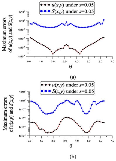
Figure 7. Showing the errors in the numerical recovery of u and S under a noise $s=0.05$, (a) example 6 and (b) example 7.

In Table 2, we consider different mesh parameters N used in the collocation method for $u(x,y)$ to influence the convergence rate as reflected in ME(S) and $e\left(S\right)$. It can be seen that more collocated points lead to a more accurate solution of S.

Table 2. For example 6, the influence of mesh parameter N on ME(S) and $e\left(S\right)$.

N	5	10	20	25	30
ME(S)	57.34	43.59	45.93	37.06	1.22
$e\left(S\right)$	$1.18\times {10}^{-1}$	$9.55\times {10}^{-2}$	$8.70\times {10}^{-2}$	$6.52\times {10}^{-2}$	$5.24\times {10}^{-3}$

8.2. Example 7

For Equation (69) with $Q=u^2+cosu$, we consider

$$u=r^2=x^2+y^2,\alpha =10+r^2+r^4{cos}^2\theta =10+(x^2+y^2)(x^2+1).$$

(71)

The outer and inner boundaries are given by Equations (62) and (63), respectively.

For this example, we have $m=2$, $N=20$ and a noise $s=5\%$, as shown in Figure 7b, the maximum absolute error of u is $2.03\times {10}^{-2}$, which is more accurate than $max\left(u\right)=18.62$. The ME of $S(x,y)$ is 1.04, which is much smaller than $maxS=4001.42$. The value $e\left(S\right)=2.99\times {10}^{-4}$ is quite small. The dimension of the normal matrix of the linear system (41) and (40) is $n_1\times n_1=4\times 4$, and the condition number is small with COND = 19.858.

In Table 3, we consider different mesh parameters of N used in the collocation method for $u(x,y)$ to influence the convergence rate as reflected in ME(S) and $e\left(S\right)$. It can be seen that more collocated points lead to a more accurate solution of S and even for a small $N=3$ the accuracy is good.

Table 3. For example 7, the influence of mesh parameter N on ME(S) and $e\left(S\right)$.

N	3	8	14	18	20
ME(S)	12.09	10.98	8.98	8.51	1.04
$e\left(S\right)$	$3.70\times {10}^{-3}$	$2.87\times {10}^{-3}$	$2.57\times {10}^{-3}$	$2.17\times {10}^{-3}$	$2.99\times {10}^{-4}$

9. Conclusions

In the paper, we have constructed a category of two-parameter homogenization functions in the 2D doubly connected domain for automatically satisfying the outer Dirichlet and Neumann boundary conditions of the nonlinear elliptic equation. A new numerical method was developed for solving the inverse problems through the technique of two-parameter homogenization functions, which include the recovery of the space-dependent and temperature-dependent conductivity functions and also the source function. We first determine $u(x,y)$ in terms of the bases and then a linear system to satisfy the inner boundary condition by the method of collocation is solved. Back-substituting the solution into the nonlinear elliptic equation, we recovered the unknown space-dependent and temperature-dependent conductivity functions by collocating points inside the domain and solving the derived linear equations. The basis $B(j,k,x,y)$ has good behavior used in the interpolation for $u(x,y)$ in a weighted Sobolev space, such that we can recover $u(x,y)$ very well; hence, after the back substitution of $u(x,y)$ into the governing equation, the source function was directly recovered with high accuracy. It maintains the same advantages of accuracy and efficiency for solving the inverse conductivity problems and inverse Robin problems, even for large noise.

References

- Tuan, N.H.; Khoa, V.A.; Tran, T. On an inverse boundary value problem of a nonlinear elliptic equation in three dimensions. J. Math. Anal. Appl. 2015, 426, 1232–1261. [Google Scholar] [CrossRef]
- Farcas, A.; Elliott, L.; Ingham, D.B.; Lesnic, D.; Mera, N.S. A dual reciprocity boundary element method for the regularized numerical solution of the inverse source problem associated to the Poisson equation. Inv. Prob. Sci. Eng. 2003, 11, 123–139. [Google Scholar] [CrossRef]
- Jin, B.T.; Marin, L. The method of fundamental solutions for inverse source problems associated with the steady-state heat conduction. Int. J. Numer. Meth. Eng. 2007, 69, 1570–1589. [Google Scholar] [CrossRef]
- Klose, A.D.; Ntziachristos, V.; Hielscher, A.H. The inverse source problem based on the radiative transfer equation in optical molecular imaging. J. Comput. Phys. 2005, 202, 323–345. [Google Scholar] [CrossRef]
- Hon, Y.C.; Li, M.; Melnikov, Y.A. Inverse source identification by Green’s function. Eng. Anal. Bound. Elem. 2010, 34, 352–358. [Google Scholar] [CrossRef]
- Li, X.X.; Guo, H.Z.; Wan, S.M.; Yang, F. Inverse source identification by the modified regularization method on Poisson equation. J. Appl. Math. 2012, 2012, 971952. [Google Scholar] [CrossRef]
- Ahmadabadi, M.N.; Arab, M.; Ghaini, F. The method of fundamental solutions for the inverse space-dependent heat source problem. Eng. Anal. Bound. Elem. 2009, 33, 1231–1235. [Google Scholar] [CrossRef]
- Slimani, S.; Medarhri, I.; Najib, K.; Zine, A. Identification of the source function for a seawater intrusion problem in unconfined aquifer. Numer. Algor. 2020, 84, 1565–1587. [Google Scholar] [CrossRef]
- Alahyane, M.; Boutaayamou, I.; Chrifi, A.; Echarroudi, Y.; Ouakrim, Y. Numerical study of inverse source problem for internal degenerate parabolic equation. Int. J. Comput. Meth. 2020, 18, 2050032. [Google Scholar] [CrossRef]
- Djennadi, S.; Shawagfeh, N.; Arqub, O.A. A fractional Tikhonov regularization method for an inverse backward and source problems in the time-space fractional diffusion equations. Chaos Solitons Fractals 2021, 150, 111127. [Google Scholar] [CrossRef]
- Ma, Y.K.; Prakash, P.; Deiveegan, A. Generalized Tikhonov methods for an inverse source problem of the time-fractional diffusion equation. Chaos Solitons Fractals 2018, 108, 39–48. [Google Scholar] [CrossRef]
- Nguyen, H.T.; Le, D.L. Regularized solution of an inverse source problem for a time fractional diffusion equation. Appl. Math. 2016, 40, 8244–8264. [Google Scholar] [CrossRef]
- Liu, C.-S. An energetic boundary functional method for solving the inverse source problems of 2D nonlinear elliptic equations. Eng. Anal. Bound. Elem. 2020, 118, 204–215. [Google Scholar] [CrossRef]
- Kwon, K. Identification of anisotropic anomalous region in inverse problems. Inverse Probl. 2004, 20, 1117–1136. [Google Scholar] [CrossRef]
- Huntul, M.J.; Lesnic, D. An inverse problem of finding the time-dependent thermal conductivity from boundary data. Int. Commun. Heat Mass Transf. 2017, 85, 147–154. [Google Scholar] [CrossRef] [Green Version]
- Isakov, V.; Sever, A. Numerical implementation of an integral equation method for the inverse conductivity problem. Inverse Probl. 1996, 12, 939–951. [Google Scholar] [CrossRef]
- Murthy, R.; Lin, Y.H.; Shin, K.; Mueller, J.L. A direct reconstruction algorithm for the anisotropic inverse conductivity problem based on Calderόn method in the plane. Inverse Probl. 2020, 12, 125008. [Google Scholar] [CrossRef]
- Liu, C.-S.; Qiu, L.; Lin, J. Simulating thin plate bending problems by a family of two-parameter homogenization functions. Appl. Math. Model. 2020, 79, 284–299. [Google Scholar] [CrossRef]
- Liu, C.-S.; Atluri, S.N. An iterative and adaptive Lie-group method for solving the Calderόn inverse problem. Comput. Model. Eng. Sci. 2010, 64, 299–326. [Google Scholar]
- Sladek, J.; Sladek, V.; Hon, Y.C. Inverse heat conduction problems by meshless local Petrov–Galerkin method. Eng. Anal. Boundary Elem. 2006, 30, 650–661. [Google Scholar] [CrossRef]
- Gu, Y.; Chen, W.; Zhang, C.; He, X. A meshless singular boundary method for three-dimensional inverse heat conduction problems in general anisotropic media. Int. J. Heat Mass Transf. 2015, 84, 91–102. [Google Scholar] [CrossRef]
- Shivanian, E.; Khodabandehlo, H.R. Application of meshless local radial point interpolation (MLRPI) on a one-dimensional inverse heat conduction problem. Ain Shams Eng. J. 2016, 7, 993–1000. [Google Scholar] [CrossRef] [Green Version]
- Sun, Y.; He, S. A meshless method based on the method of fundamental solution for three-dimensional inverse heat conduction problems. Int. J. Heat Mass Transf. 2017, 108, 945–960. [Google Scholar] [CrossRef]
Publisher’s Note: MDPI stays neutral with regard to jurisdictional claims in published maps and institutional affiliations. |
© 2022 by the authors. Licensee MDPI, Basel, Switzerland. This article is an open access article distributed under the terms and conditions of the Creative Commons Attribution (CC BY) license (https://creativecommons.org/licenses/by/4.0/).