Identifying the Unknown Source in Linear Parabolic Equation by a Convoluting Equation Method

Abstract

This article is devoted to identifying a space-dependent source term in linear parabolic equations. Such a problem is ill posed, i.e., a small perturbation in the input data may cause a dramatically large error in the solution (if it exists). The conditional stability of the solution is analyzed. Based on a convoluting equation method, we can deal with the problem under the a priori parameter choice rule. Meanwhile, a modified version of Morozov’s discrepancy principle is provided to decide on an a posteriori regularization parameter choice strategy and a log-type error estimate is obtained. Two numerical results show that our proposed method works well.

1. Introduction

It is an important natural process of transport and diffusion and the following parabolic partial differential equation is induced

$$u_t+Lu=f(x,t;u),(x,t)\in \mathsf{\Omega }\times (0,T),$$

(1)

where $\mathsf{\Omega }$ is a bounded domain in ${\mathbb{R}}^d(1\le d\le 3)$, u represents the state variable, L is a differential operator with respect to x, such as the second order elliptic operator $Lu=-(u_{xx}+v{u}_x-qu)$ with fixed constants $v,q$ and the space-fractional diffusion operator $Lu={-}_x{D}_{\theta }^{\alpha }$, and f denotes some physical laws.

In many branches of science and engineering, e.g., crack identification, geophysical prospecting, pollutant detection, and also for designing the final state in melting and freezing processes, the characteristics of sources are often unknown and need to be determined. This is the so-called inverse source identification problem , which is a classic ill-posed problem in the sense of Hadamard, i.e., a small perturbation in the input data may cause a dramatically large error in the solution (if it exists). Many studies on such inverse problems of determining source terms have been performed since the 1970s. There have been a large number of research results for different forms of heat sources [1,2,3,4,5,6,7,8,9,10,11]. A few theoretical articles concern conditional stability and the data compatibility of the solution notably in [1,3,8,12,13,14,15]. As yet, there are many published works in this field based in several numerical methods, such as the Lie-group shooting method (LGSM) [5], the coupled method [16], the fundamental solutions method [6,17], the meshless method [7,18], the genetic algorithm [4], and the conjugate gradient method (CGM) [19,20,21]. In [22,23], these numerical methods were considered to solve two and three-dimensional inverse transient heat source problems. In [24], the authors used the simplified Tikhonov method to identify the unknown source. There are some other the regularization methods to solve this problem, such as the Fourier regularization method [25], the wavelet dual squares method [26], the Tikhonov-type method [27], the mollification regularization method [10,11,28], the optimization method [29], and the Landweber method [30,31].

Although many different numerical schemes have been introduced in recent decades to solve the inverse source identification problem, it has not completely been solved yet. Based on some of the traditional methods, finite differences method (FDM) [32], finite element method (FEM), and the boundary element method (BEM) [2,33], the inverse source identification problem has been solved. Furthermore, other methods such as the linear least-squares error method, the sequential method, and the iterative regularization methods [20,34,35] have been used to deal with the inverse source problem. As for these methods, it is necessary for us to discretize the differential equations. However, the ill posing of these kinds of problems and the ill conditioning of the resulting discretized matrix are the main problems in constructing the numerical algorithm for determining these problems. Therefore, a suitable regularization method should be used.

In this article, we prefer to use a convoluting equation method to consider the identification of the unknown source problem. The idea was borrowed from [36], where Zheng and Wei proposed a modified equation method using convolution to solve the space-fractional backward diffusion problem. At present, there are few studies using this regularization method [36,37,38]. In [37], Cong Shi and his coauthors used this method, which they called the convolution regularization, to solve the backward problems of linear parabolic equations. In [38], the authors studied the a posteriori parameter choice of this method for the space-fractional backward diffusion problem. However, the a posteriori choice of the regularization parameter is not given in [36]. The conditional stability of the corresponding problem is not discussed in the above literature. This article can be regarded as an extension of the above work. The difference is that the Refs. [36,37,38] are devoted to the backward problem. The present article is devoted to the inverse source identification problem. In fact, this article is devoted to three aspects: (1) The conditional stability for the IHSP is considered under a suitable priori condition in Section 2; (2) The a priori strategy for choosing the regularization parameter and the corresponding error estimate is given; (3) We do an analysis on the fact that the Morozov’s discrepancy principle does not work here and give a new a posteriori parameter choice based on a modified version of the discrepancy principle; we also obtain a log-type error estimate under an additional source condition.

The techniques in this article may also be applied to other inverse problems, such as the high-dimensional cases or elliptic partial differential equations, which is also our next research work. It is worth pointing out that the convoluting equation method in this article is different from the mollification method [10,11,28]. The mollification method is to use a convolution of the noise data and a smooth function with a parameter to filter the high-frequency components of the noise data. The convoluting equation method is to prevent the high-frequency components of the solution from blowing up by convolution with the derivative term of space in the equation.

The outline of this article is as follows. Section 2 analyzes the ill posedness of the inverse heat source problem and its conditional stability. In Section 3, the convoluting equation method is given, and we derive the convergence rates under the a priori rules for the choices of the regularization parameter. In Section 4, we come up with a new generalized discrepancy principle to decide the regularization parameter. Section 5 gives two numerical examples to demonstrate the reasonableness and effectiveness under two kinds of regularization parameter choice rules. Section 6 concludes the article and gives some suggestions.

2. Mathematical Formulation, Ill Posedness of the Problem, and Its Conditional Stability

We consider the one-dimensional problem in which the source term $f(x,t;u)=f(x)$ depends on just space parameter and satisfies

$$\left\{\begin{array}{cc}{u}_t(x,t)+Lu(x,t)=f(x),\hfill & x\in \mathbb{R},t>0,\hfill \\ u(x,0)=0,\hfill & x\in \mathbb{R},\hfill \\ u(x,T)=g(x),\hfill & x\in \mathbb{R}.\hfill \end{array}\right.$$

(2)

where $g(x)$ is given and $f(x)$ is unknown. In practice, the exact data g is always unknown and we only have a noisy measurement $g^{\delta }\in L^2(\mathbb{R})$. We use the additional data $u(x,T)=g^{\delta }(x)$ to identify the source term $f(x)$.

In order to analyze the problem (2) in $L^2(\mathbb{R})$, we let $\parallel ·\parallel$ denote the norm in $L^2(\mathbb{R})$, and

$$\widehat{f}(\xi ):=\frac{1}{\sqrt{2\pi }}{\int }_{-\infty }^{\infty }{e}^{-i\xi x}f(x)dx$$

(3)

represent the Fourier transform of the function $f(x)$.

We define the operator L as a differential operator or a fractional differential operator with respect to $x\in \mathbb{R}$, which is given by the Fourier transform

$$\widehat{L}u(\xi ,t)=l(\xi )\widehat{u}(\xi ,t)$$

(4)

and $l:\mathbb{R}\to \mathbb{C}$ is a function called the symbol of the operator L, satisfying the following conditions:

$$(L_1)|l(\xi )|\le a_1{(1+|\xi |}^{\alpha }),\xi \in \mathbb{R},a_1>0,\alpha >0;$$

$$(L_2)Re(l(\xi ))\ge a_2{|\xi |}^{\alpha },\xi \in \mathbb{R},a_2>0,\alpha >0.$$

where $\alpha >0$ is the order of the operator L. Here are some examples in the following forms:

• If $Lu=-u_{xx}$, then $u_t=u_{xx}+f(x)$, where $l(\xi )={\xi }^2$ for $\alpha =2$.
• If $Lu=-u_{xx}-v{u}_x+qu$, then $u_t=u_{xx}+v{u}_x-qu+f(x)$, the constant $v,q\ge 0$ where $l(\xi )={\xi }^2-i\xi v+q$ for $\alpha =2$.
• If $Lu=-{}_x{D}_{\theta }^{\alpha }u$, then $u_t={}_x{D}_{\theta }^{\alpha }u+f(x)$, where the space-factional derivative ${}_x{D}_{\theta }^{\alpha }u(x,t)$, which is the Riesz-Feller fractional derivative of order
  $\alpha (0<\alpha \le 2)$ and skewness $\theta (|\theta |\le min(\alpha ,2-\alpha ),\theta \ne \pm 1)$, is defined in terms of the Fourier transform in [39], i.e.,

  $$\mathcal{F}{\{}_x{D}_{\theta }^{\alpha }f(x);\xi \}=-{\psi }_{\theta }^{\alpha }(\xi )\widehat{f}(\xi ),$$

  (5)

  where ${\psi }_{\theta }^{\alpha }(\xi )={|\xi |}^{\alpha }{e}^{i(sgn\xi )\theta \pi /2}$, this is, $l(\xi )={|\xi |}^{\alpha }{e}^{i(sgn\xi )\theta \pi /2}$.

According to the equation and the initial value in (2), we can obtain the solution in frequency domain

$$\widehat{u}(\xi ,t)=\frac{1-e^{-l(\xi )t}}{l(\xi )}\widehat{f}(\xi ).$$

(6)

By using the additional data in (2), we obtain

$$\widehat{f}(\xi )=\frac{l(\xi )}{1-e^{-Tl(\xi )}}\widehat{g}(\xi ),$$

(7)

or equivalently,

$$f(x)=\frac{1}{\sqrt{2\pi }}{\int }_{-\infty }^{\infty }{e}^{i\xi x}\frac{l(\xi )\widehat{g}(\xi )}{1-e^{-Tl(\xi )}}d\xi .$$

(8)

Furthermore, setting $\widehat{K}=\frac{1-e^{-Tl(\xi )}}{l(\xi )}:L^2(\mathbb{R})\to L^2(\mathbb{R})$ is a multiplication operator in the frequency domain, we have $\widehat{K}\widehat{f}=\widehat{g}$.

Our purpose is to identify $f(x)$ from the noise data $g^{\delta }(x)$. However, when $\xi \to \infty$, the function $\frac{l(\xi )}{1-e^{-Tl(\xi )}}$ is unbounded. Therefore, it can be considered to be an amplified factor with respect variable $\xi$ for fixed $\alpha >0$. The source term $f(x)$ is assumed to be in $L^2(\mathbb{R})$; then, the exact data function $\widehat{g}(\xi )$ must decay as $\xi \to \infty$. However, the noisy data function $g^{\delta }(x)$, which is only in $L^2(\mathbb{R})$, does not have the same decay in the frequency domain. So, this problem is mildly ill posed and the degree of the ill posedness is equivalent to that of the $\alpha$-order numerical differentiation. We will deal with the ill-posed problem via a convoluting equation method in the next section.

Lemma 1.

If $x>1$, the following inequality holds

$$\frac{1}{1-e^{-x}}<2.$$

The proof of Lemma 1 is straightforward, so we omit it here.

Lemma 2.

If $z=x+iy$ for $x\ge 0$ and $y\in \mathbb{R}$, then we can obtain $|1-e^{-z}|\le min\{2,2|z|\}$.

Proof. 

Due to the inequality that $|1-e^{-z}|\le 1+|e^{-z}|\le 2$, and

$$\begin{array}{cc}\hfill |1-e^{-z}|& \le |1-e^{-iy}|+|e^{-iy}-e^{-x-iy}|\le |y|+x\le 2|z|.\hfill \end{array}$$

Because the problem (2) is linear, we can derive the following conditional stability estimate on the solution when the data function $g(x)$ is close to zero. □

Theorem 1.

If ${\parallel f(x)\parallel }_p\le E$, then the following estimate holds

$$\parallel f(x)\parallel \le 2^{\frac{p}{p+\alpha }}max\{(a_1(1+|{\xi }_0{|}^{-\alpha }{))}^{\frac{p}{p+\alpha }},T^{-\frac{p}{p+\alpha }}\}{E}^{\frac{\alpha }{p+\alpha }}{\parallel g\parallel }^{\frac{p}{p+\alpha }},$$

where ${\parallel ·\parallel }_p$ refers to the $H^p$ norm, ${\xi }_0$ satisfy $|l({\xi }_0)|=\frac{1}{T}$.

Proof. 

From (7), Parseval formula and Hölder inequality, we have

$$\begin{array}{cc}\hfill {\parallel f(x)\parallel }^2& =\parallel \widehat{f}{(\xi )\parallel }^2={\int }_{-\infty }^{\infty }(\frac{l(\xi )}{1-e^{-Tl(\xi )}}{)}^2\widehat{g}{(\xi )}^{2}d\xi \hfill \\ \hfill & ={\int }_{-\infty }^{\infty }(\frac{l(\xi )}{1-e^{-Tl(\xi )}}{)}^2\widehat{g}{(\xi )}^{\frac{2\alpha }{p+\alpha }}\widehat{g}{(\xi )}^{\frac{2p}{p+\alpha }}d\xi \hfill \\ \hfill & \le ({\int }_{-\infty }^{\infty }(\frac{l(\xi )}{1-e^{-Tl(\xi )}}{)}^{\frac{2(p+\alpha )}{\alpha }}\widehat{g}{(\xi )}^{2}d\xi {)}^{\frac{\alpha }{p+\alpha }}({\int }_{-\infty }^{\infty }\widehat{g}{(\xi )}^{2}d\xi {)}^{\frac{p}{p+\alpha }}\hfill \\ \hfill & =({\int }_{-\infty }^{\infty }(\frac{l(\xi )}{1-e^{-Tl(\xi )}}{)}^{\frac{2p}{\alpha }}{(1+{\xi }^2)}^{-p}{(1+{\xi }^2)}^p(\frac{l(\xi )\widehat{g}(\xi )}{1-e^{-Tl(\xi )}}{)}^{2}d\xi {)}^{\frac{\alpha }{p+\alpha }}{\parallel g\parallel }^{\frac{2p}{p+\alpha }}\hfill \\ \hfill & \le (\underset{\xi \in \mathbb{R}}{sup}(\frac{|l(\xi )|}{1-e^{-T|l(\xi )|}}{)}^{\frac{2p}{\alpha }}{(1+{\xi }^2)}^{-p}{)}^{\frac{\alpha }{p+\alpha }}{E}^{\frac{2\alpha }{p+\alpha }}{\parallel g\parallel }^{\frac{2p}{p+\alpha }}.\hfill \end{array}$$

Due to $|l(\xi )|$ tending to infinity as $|\xi |\to \infty$, there must exist a ${\xi }_0$, satisfying $|Tl(\xi )|=1$. Furthermore, we know $|l(\xi )|$ is an increasing function with respect to $|\xi |$. If we let

$$H(\xi )={(\frac{|l(\xi )|}{1-e^{-T|l(\xi )|}})}^{\frac{2p}{\alpha }}{(1+{\xi }^2)}^{-p},$$

so when $\xi >{\xi }_0$, this is, $|Tl(\xi )|>1$, then by Lemma 1 and $(L_1)$ we have

$$H(\xi )\le {(2a_1)}^{\frac{2p}{\alpha }}{(1+|\xi |}^{\alpha }{)}^{\frac{2p}{\alpha }}{\xi }^{-2p}\le {(2a_1)}^{\frac{2p}{\alpha }}(1+{|{\xi }_0|}^{-\alpha }{)}^{\frac{2p}{\alpha }}.$$

When $0<\xi \le {\xi }_0$, thus $|Tl(\xi )|\le 1$, note that $H(\xi )$ is also an increasing function with respect to $\xi$, then, we have

$$H(\xi )\le H({\xi }_0)\le (\frac{|l({\xi }_0)|}{1-e^{-T|l({\xi }_0)|}}{)}^{\frac{2p}{\alpha }}\le (\frac{2}{T}{)}^{\frac{2p}{\alpha }}.$$

From the above two cases, the proof of Theorem 1 is completed. □

Remark 1.

If $f_1(x)$ and $f_2(x)$ denote, respectively, the corresponding source terms of any given functions $g_1(x)$ and $g_2(x)$ in problem (2), then we have

$$\parallel f_1(x)-f_2(x)\parallel \le 2^{\frac{p}{p+\alpha }}max\{(a_1(1+|{\xi }_0{|}^{-\alpha }{))}^{\frac{p}{p+\alpha }},T^{-\frac{p}{p+\alpha }}\}{E}^{\frac{\alpha }{p+\alpha }}{\parallel g_1(x)-g_2(x)\parallel }^{\frac{p}{p+\alpha }},$$

where ${\xi }_0$ satisfy $|l({\xi }_0)|=\frac{1}{T}$.

3. Convoluting Equation Method and Its Convergence Analysis under a Priori Parameter Choice Rule

By modifying Equation (2) as the following, we can obtain an approximate solution for (2), i.e.,

$$\left\{\begin{array}{cc}{u}_t(x,t)+P_{\mu }(x)\ast Lu(x,t)=f(x),\hfill & x\in \mathbb{R},t>0,\hfill \\ u(x,0)=0,\hfill & x\in \mathbb{R},\hfill \\ u(x,T)=g^{\delta }(x),\hfill & x\in \mathbb{R}.\hfill \end{array}\right.$$

(9)

where “*” denotes the convolution operation, $P_{\mu }(x)$ is called kernel function, and $\mu$ is the regularization parameter. In reality, the measurement data are noise contaminated and satisfy

$$\parallel g(x)-g^{\delta }(x)\parallel \le \delta ,$$

(10)

where the level of tolerance $\delta >0$ represents a bound on the measurement error and $\parallel ·\parallel$ refers to the $L^2$-norm.

If using Fourier transform (3), the solution of problem (9) can be formulated in the frequency space as follows:

$${\widehat{f}}_{\mu }^{\delta }(\xi )=\frac{{\widehat{P}}_{\mu }(\xi )l(\xi )}{1-e^{-T{\widehat{P}}_{\mu }(\xi )l(\xi )}}{\widehat{g}}^{\delta }(\xi ).$$

(11)

The suitable convolution kernel $P_{\mu }(x)$ must satisfy the following two conditions:

• For each fixed $\mu >0$, $\frac{{\widehat{P}}_{\mu }(\xi )l(\xi )}{1-e^{-T{\widehat{P}}_{\mu }(\xi )l(\xi )}}$ is bounded as $|\xi |\to \infty$.
• If $\xi$ is fixed, then $\frac{{\widehat{P}}_{\mu }(\xi )l(\xi )}{1-e^{-T{\widehat{P}}_{\mu }(\xi )l(\xi )}}\to \frac{l(\xi )}{1-e^{-Tl(\xi )}}$ as $\mu \to 0$.

Due to the fact that the proposed method aims to filter the smaller singular values for the linear self-adjoint compact operator $\widehat{K}$, we suppose that the convolution kernels satisfy three properties, as follows.

Definition 1.

A family of functions ${P_{\mu }(x)}_{\mu >0}$ is called a regularization kernel of order $(\alpha ,\beta )$ for $\alpha ,\beta >0$, if the following three properties are satisfied for all $\xi \in \mathbb{R}$,

$(K_1)0\le {\widehat{P}}_{\mu }(\xi )\le 1$;

$(K_2)|1-{\widehat{P}}_{\mu }(\xi )|\le b_1{|\mu \xi |}^{\beta },b_1>0$ is a constant;

$(K_3){\widehat{P}}_{\mu }(\xi ){|\xi |}^{\alpha }\le b_2{\mu }^{-\alpha },b_2>0$ is a constant.

In this article, we will give some possible convolution kernels:

Case 1. The kernel $P_{\mu }(x)=\frac{e^{-\frac{|x|}{\mu }}}{2\mu }$ (see [36]), and its Fourier transform is ${\widehat{P}}_{\mu }(\xi )=\frac{1}{1+{\mu }^2{\xi }^2}$, the kernel is of order $(\alpha ,2)$ for $0<\alpha \le 2$.

Case 2. The kernel $P_{\mu }(x)=\frac{1}{2\sqrt{\pi }\mu }{e}^{-\frac{x^2}{4{\mu }^2}}$, and ${\widehat{P}}_{\mu }(\xi )=e^{-{\mu }^2{\xi }^2}$, the kernel is of order $(\alpha ,2)$ for any $\alpha >0$.

Case 3. If making the above two cases generalization, we have ${\widehat{P}}_{\mu }(\xi )=\frac{1}{1+{(\mu |\xi |)}^{\beta }}$ or ${\widehat{P}}_{\mu }(\xi )=e^{-{(\mu |\xi |)}^{\beta }}$ which have order $(\alpha ,\beta )$ for $0<\alpha \le \beta$.

Case 4. We could also choose $P_{\mu }(x)=\frac{1}{\pi x}sin\frac{x}{\mu }$, which gives ${\widehat{P}}_{\mu }(\xi )={\chi }_{[-\frac{1}{\mu },\frac{1}{\mu }]}(\xi )$, and the kernel is of order $(\alpha ,\beta )$ for any $\beta \ge 1$ and $\alpha >0$.

Now, let us verify that Case 1 to Case 4 satisfy the conditions in Definition 1. It is obvious to prove the $(K_1)$ for all cases above. Note that $1-\frac{1}{1+{(\mu |\xi |)}^{\beta }}=\frac{{(\mu |\xi |)}^{\beta }}{1+{(\mu |\xi |)}^{\beta }}\le {(\mu |\xi |)}^{\beta }$, $1-e^{-{(\mu |\xi |)}^{\beta }}\le {(\mu |\xi |)}^{\beta }$, we have verified the $(K_2)$. As for $(K_3)$, we have $\frac{{(\mu |\xi |)}^{\alpha }}{1+{(\mu |\xi |)}^{\beta }}\le 1$ for $0<\alpha \le \beta$, then $\frac{{|\xi |}^{\alpha }}{1+{(\mu |\xi |)}^{\beta }}\le {\mu }^{-\alpha },{\mu }^{\alpha }{|\xi |}^{\alpha }{e}^{-{(\mu |\xi |)}^{\beta }}\le {(\frac{\alpha }{e\beta })}^{\frac{\alpha }{\beta }}\le 1$, then we also have $e^{-{(\mu |\xi |)}^{\beta }}{|\xi |}^{\alpha }\le {\mu }^{-\alpha }$.

According to the knowledge of Sobolev Space, we use the following assumption here

$${\parallel f(x)\parallel }_p:= ({\int }_{-\infty }^{\infty }{(1+{\xi }^2)}^p|\widehat{f}(\xi ){{|}^{2}d\xi )}^{\frac{1}{2}}\le E,p>0.$$

(12)

(A) (Stability). Set $f_{\mu }(x)$ is the solution of (9) with $\delta =0$, i.e.,

$${\widehat{f}}_{\mu }(\xi )=\frac{{\widehat{P}}_{\mu }(\xi )l(\xi )}{1-e^{-T{\widehat{P}}_{\mu }(\xi )l(\xi )}}\widehat{g}(\xi ).$$

Due to the Parseval identity, we have

$$\begin{array}{cc}\hfill \parallel f_{\mu }^{\delta }(x)-f_{\mu }(x)\parallel & =\parallel {\widehat{f}}_{\mu }^{\delta }(\xi )-{\widehat{f}}_{\mu }(\xi )\parallel \hfill \\ \hfill & =\parallel \frac{{\widehat{P}}_{\mu }(\xi )l(\xi )}{1-e^{-T{\widehat{P}}_{\mu }(\xi )l(\xi )}}({\widehat{g}}^{\delta }(\xi )-\widehat{g}(\xi ))\parallel \hfill \\ \hfill & \le \delta \underset{\xi \in \mathbb{R}}{sup}\frac{|{\widehat{P}}_{\mu }(\xi )l(\xi )|}{1-e^{-T|{\widehat{P}}_{\mu }(\xi )l(\xi )|}}.\hfill \end{array}$$

Let $G(\xi )=\frac{|{\widehat{P}}_{\mu }(\xi )l(\xi )|}{1-e^{-T|{\widehat{P}}_{\mu }(\xi )l(\xi )|}}$, if $s=|{\widehat{P}}_{\mu }(\xi )l(\xi )|$, then $G(\xi )$ can be rewritten as $G(s):=\frac{s}{1-e^{-Ts}}$, which is an increasing function with respect to s. From $(L_1),(K_1)$, $(K_3)$, and Lemma 1, we obtain

$$G(\xi )\le 2a_1(1+b_2{\mu }^{-\alpha }).$$

Combining with the above inequality, we have

$$\parallel f_{\mu }^{\delta }(x)-f_{\mu }(x)\parallel \le 2a_1(1+b_2{\mu }^{-\alpha })\delta .$$

(13)

(B) (Convergence). From the Parseval identity, we have

$$\begin{array}{cc}\hfill \parallel f_{\mu }(x)-f(x)\parallel & =\parallel {\widehat{f}}_{\mu }(\xi )-\widehat{f}(\xi )\parallel =\parallel \frac{{\widehat{P}}_{\mu }(\xi )l(\xi )}{1-e^{-T{\widehat{P}}_{\mu }(\xi )l(\xi )}}\widehat{g}(\xi )-\widehat{f}(\xi )\parallel \hfill \\ \hfill & =\parallel (1-\frac{{\widehat{P}}_{\mu }(\xi )(1-e^{-Tl(\xi )})}{1-e^{-T{\widehat{P}}_{\mu }(\xi )l(\xi )}})\widehat{f}(\xi )\parallel \hfill \\ \hfill & \le \underset{\xi \in \mathbb{R}}{sup}|(1-\frac{{\widehat{P}}_{\mu }(\xi )(1-e^{-Tl(\xi )})}{1-e^{-T{\widehat{P}}_{\mu }(\xi )l(\xi )}}){(1+{\xi }^2)}^{-\frac{p}{2}}|\parallel {(1+{\xi }^2)}^{\frac{p}{2}}\widehat{f}(\xi )\parallel \hfill \\ \hfill & \le E\underset{\xi \in \mathbb{R}}{sup}|(1-\frac{{\widehat{P}}_{\mu }(\xi )(1-e^{-T|l(\xi )|})}{1-e^{-T{\widehat{P}}_{\mu }(\xi )|l(\xi )|}}){(1+{\xi }^2)}^{-\frac{p}{2}}|.\hfill \end{array}$$

Let $D(\xi )=(1-\frac{{\widehat{P}}_{\mu }(\xi )(1-e^{-T|l(\xi )|})}{1-e^{-T{\widehat{P}}_{\mu }(\xi )|l(\xi )|}}){(1+{\xi }^2)}^{-\frac{p}{2}}$, we divide $D(\xi )$ into two cases:

Case 1. $|\xi |>{\mu }^{-\gamma }$, we have

$$D(\xi )\le (1-{\widehat{P}}_{\mu }(\xi )){|\xi |}^{-p}\le {\mu }^{p\gamma }.$$

Case 2. $|\xi |\le {\mu }^{-\gamma }$, we have

$$\begin{array}{cc}\hfill D(\xi )& \le 1-\frac{{\widehat{P}}_{\mu }(\xi )(1-e^{-T|l(\xi )|})}{1-e^{-T{\widehat{P}}_{\mu }(\xi )|l(\xi )|}}\hfill \\ \hfill & \le 1-{\widehat{P}}_{\mu }(\xi )\le b_1{|\mu \xi |}^{\beta }\le b_1{\mu }^{(1-\gamma )\beta }.\hfill \end{array}$$

If we choose $\gamma =\frac{\beta }{p+\beta }$, then we can obtain

$$D(\xi )\le max\{1,b_1\}{\mu }^{\frac{p\beta }{p+\beta }}.$$

Thus

$$\parallel f_{\mu }(x)-f(x)\parallel \le max\{1,b_1\}{\mu }^{\frac{p\beta }{p+\beta }}E.$$

(14)

Combining (A) and (B) and using Parseval identity, we finally obtain the following error estimation.

Theorem 2.

Assume that $P_{\mu }(x)$ is the convolution kernel of order $(\alpha ,\beta ),0<\alpha \le \beta .$ If the regularized solution given in (11) with noisy data $g^{\delta }(x)$ satisfies (10) and (12) and $\mu ={(\frac{\delta }{E})}^{\frac{p+\beta }{p\beta +\alpha (p+\beta )}}$ which is selected to be a regularization parameter, then we have

$$\parallel f_{\mu }^{\delta }(x)-f(x)\parallel \le C_1{\delta }^{\frac{p\beta }{p\beta +\alpha (p+\beta )}}{E}^{\frac{\alpha (p+\beta )}{p\beta +\alpha (p+\beta )}},$$

where $C_1,\alpha ,\beta ,p>0$ are constants and $0<\alpha \le \beta$.

Proof. 

From the Parseval identity and the triangle inequality, we obtain

$$\parallel f_{\mu }^{\delta }(x)-f(x)\parallel =\parallel {\widehat{f}}_{\mu }^{\delta }(\xi )-\widehat{f}(\xi )\parallel \le \parallel {\widehat{f}}_{\mu }^{\delta }(\xi )-{\widehat{f}}_{\mu }(\xi )\parallel +\parallel {\widehat{f}}_{\mu }(\xi )-\widehat{f}(\xi )\parallel .$$

(15)

Combining (13)–(15), we know

$$\begin{array}{cc}\hfill \parallel f_{\mu }^{\delta }(x)-f(x)\parallel & \le 2a_1(1+b_2{\mu }^{-\alpha })\delta +max\{1,b_1\}{\mu }^{\frac{p\beta }{p+\beta }}E\hfill \\ \hfill & \le 2a_1\delta +(2a_1{b}_2+max\{1,b_1\})E^{\frac{\alpha (p+\beta )}{p\beta +\alpha (p+\beta )}}{\delta }^{\frac{p\beta }{p\beta +\alpha (p+\beta )}}.\hfill \end{array}$$

Set $C_1=2a_1{b}_2+max\{1,b_1\}$, when $\delta$ is sufficiently small, the estimate is satisfied. The proof of Theorem 2 is completed. □

4. The New Discrepancy Principle

In this section, we will discuss an a posteriori choice rule for the regularization parameter. We recall the definition of Morozov’s discrepancy principle for our case, which is to find $\mu$ such that

$$\parallel \widehat{K}{\widehat{f}}_{\mu }^{\delta }(\xi )-{\widehat{g}}^{\delta }(\xi )\parallel =\tau \delta ,$$

where $\tau >2$ (large enough) is a fixed constant.

However, in the convoluting equation method, by the Morozov’s discrepancy principle, we obtain

$$\begin{array}{cc}\hfill \tau \delta & =\parallel \widehat{K}{\widehat{f}}_{\mu }^{\delta }(\xi )-{\widehat{g}}^{\delta }(\xi )\parallel \hfill \\ \hfill & \le \parallel \widehat{K}{\widehat{f}}_{\mu }^{\delta }(\xi )-\widehat{K}{\widehat{f}}_{\mu }(\xi )\parallel +\parallel \widehat{K}{\widehat{f}}_{\mu }(\xi )-\widehat{g}(\xi )\parallel +\parallel \widehat{g}(\xi )-{\widehat{g}}^{\delta }(\xi )\parallel \hfill \\ \hfill & \le \delta \underset{\xi \in \mathbb{R}}{sup}\frac{1-e^{-T|l(\xi )|}}{|l(\xi )|}\frac{{\widehat{P}}_{\mu }(\xi )|l(\xi )|}{1-e^{-T{\widehat{P}}_{\mu }(\xi )|l(\xi )|}}+\parallel \widehat{K}{\widehat{f}}_{\mu }(\xi )-\widehat{K}\widehat{f}(\xi )\parallel +\delta .\hfill \end{array}$$

Let $A(\xi )=\frac{1-e^{-T|l(\xi )|}}{|l(\xi )|}\frac{{\widehat{P}}_{\mu }(\xi )|l(\xi )|}{1-e^{-T{\widehat{P}}_{\mu }(\xi )|l(\xi )|}},B(\xi )=\frac{{\widehat{P}}_{\mu }(\xi )|l(\xi )|}{1-e^{-T{\widehat{P}}_{\mu }(\xi )|l(\xi )|}}.$ Setting $s={\widehat{P}}_{\mu }(\xi )|l(\xi )|$, due to $(K_1)$, we have $0<s\le |l(\xi )|$. Thus, $B(\xi )$ can be rewritten as $B(s):=\frac{s}{1-e^{-Ts}}$, it is straightforward that $B(s)$ is a strictly increasing function. Then, we can obtain

$$B(s)\le B(|l(\xi )|)=\frac{|l(\xi )|}{1-e^{-T|l(\xi )|}}.$$

So

$$A(\xi )=\frac{1-e^{-T|l(\xi )|}}{|l(\xi )|}B(\xi )\le 1.$$

(16)

According to (16), (14) and Lemma 2, we obtain

$$\tau \delta \le 2\delta +2Tmax\{1,b_1\}{\mu }^{\frac{p\beta }{p+\beta }}E,$$

thus we merely obtain $\mu \ge C_2{\delta }^{\frac{p+\beta }{p\beta }}$, where $C_2={(\frac{\tau -2}{2ETmax\{1,b_1\}})}^{\frac{p+\beta }{p\beta }}$.

From (13), we know

$$\parallel f_{\mu }^{\delta }(x)-f_{\mu }(x)\parallel \le 2a_1(1+b_2{\mu }^{-\alpha })\delta \le 2a_1\delta +2a_1{b}_2{C}_2^{-\alpha }{\delta }^{\frac{p\beta -\alpha (p+\beta )}{p\beta }}.$$

(17)

When $\delta \to 0$, we do not know whether the right hand side of (17) tends to 0. If $p\beta >\alpha (p+\beta )$, the above inequality tends to 0 as $\delta \to 0$. If $p\beta \le \alpha (p+\beta )$, the above inequality does not tend to 0 as $\delta \to 0$. Thus, Morozov’s discrepancy principle does not work here.

In this article, we introduce a new generalized discrepancy principle as follows:

$${\mu }_D=sup\{\mu >0\mid \parallel \widehat{K}{\widehat{f}}_{\mu }^{\delta }(\xi )-{\widehat{g}}^{\delta }(\xi )\parallel \le \tau h(\delta )\},$$

(18)

where the constant $\tau >2$ (large enough), $h(\delta )={(log\frac{1}{\delta })}^{-\frac{\sigma \beta }{\alpha }}$, $\sigma \in (0,1)$, which satisfies $h(\delta )\ge \delta$ when $\delta$ is sufficiently small. Before we proceed to the actual estimation, we need to guarantee the existence of the parameter $\mu$ for (18). Because ${lim}_{\mu \to 0}{\widehat{P}}_{\mu }(\xi )=1$, then ${lim}_{\mu \to 0}\parallel \widehat{K}{\widehat{f}}_{\mu }^{\delta }(\xi )-{\widehat{g}}^{\delta }(\xi )\parallel =\parallel {\widehat{g}}^{\delta }(\xi )-{\widehat{g}}^{\delta }(\xi )\parallel =0<\tau h(\delta )$. Therefore, ${\mu }_D$ always exists whether it is a finite positive number or infinity.

If ${\mu }_D=+\infty$, we have ${lim}_{\mu \to +\infty }{\widehat{P}}_{\mu }(\xi )=0$. Furthermore, there is

$$\underset{\mu \to +\infty }{lim}\parallel \widehat{K}{\widehat{f}}_{\mu }^{\delta }(\xi )-{\widehat{g}}^{\delta }(\xi )\parallel =\parallel \widehat{K}{\widehat{g}}^{\delta }(\xi )-{\widehat{g}}^{\delta }(\xi )\parallel \le \tau h(\delta ).$$

(19)

For this case, we define ${\widehat{f}}_{{\mu }_D}^{\delta }(\xi )={\widehat{g}}^{\delta }(\xi )$ so that it always satisfies (19) in regard to whether ${\mu }_D$ is finite or not.

In the following, we will seek to bound $\mu$ from below by using the new discrepancy principle.

Lemma 3.

If $P_{\mu }(x)$ is a regularization kernel of order $(\alpha ,\beta )$, and the a priori condition (12) holds, then we can have

$$\parallel \widehat{K}{\widehat{f}}_{\mu }(\xi )-\widehat{g}(\xi )\parallel \le C_3{\mu }^{\frac{p\beta }{p+\beta }},$$

where $C_3=2Tmax\{1,b_1\}$ is a constant.

Proof. 

From the former definition in Section 2, then we know

$$\begin{array}{cc}\hfill \parallel \widehat{K}{\widehat{f}}_{\mu }(\xi )-\widehat{g}(\xi )\parallel & =\parallel \frac{1-e^{-Tl(\xi )}}{l(\xi )}\frac{{\widehat{P}}_{\mu }(\xi )l(\xi )}{1-e^{-T{\widehat{P}}_{\mu }(\xi )l(\xi )}}\widehat{g}(\xi )-\widehat{g}(\xi )\parallel \hfill \\ \hfill & =\parallel (1-\frac{{\widehat{P}}_{\mu }(\xi )(1-e^{-Tl(\xi )})}{1-e^{-T{\widehat{P}}_{\mu }(\xi )l(\xi )}})\frac{1-e^{-Tl(\xi )}}{l(\xi )}\widehat{f}(\xi ){(1+{\xi }^2)}^{\frac{p}{2}}{(1+{\xi }^2)}^{-\frac{p}{2}}\parallel \hfill \\ \hfill & \le \underset{\xi \in \mathbb{R}}{sup}|(1-\frac{{\widehat{P}}_{\mu }(\xi )(1-e^{-Tl(\xi )})}{1-e^{-T{\widehat{P}}_{\mu }(\xi )l(\xi )}})\frac{1-e^{-Tl(\xi )}}{l(\xi )}{(1+{\xi }^2)}^{-\frac{p}{2}}|\parallel {(1+{\xi }^2)}^{\frac{p}{2}}\widehat{f}(\xi )\parallel \hfill \\ \hfill & \le E\underset{\xi \in \mathbb{R}}{sup}|D(\xi )\frac{1-e^{-Tl(\xi )}}{l(\xi )}|.\hfill \end{array}$$

According to Lemma 2 and (B), we have

$$\parallel \widehat{K}{\widehat{f}}_{\mu }(\xi )-\widehat{g}(\xi )\parallel \le 2TEmax\{1,b_1\}{\mu }^{\frac{p\beta }{p+\beta }}.$$

□

Lemma 4.

Assume ${\mu }_D$ is chosen by the generalized discrepancy principle (18), and the a priori condition (12) holds. Therefore, we can obtain

$${\mu }_D\ge (\frac{(\tau -2)h(\delta )}{C_3{2}^{\frac{p\beta }{p+\beta }}}{)}^{\frac{p+\beta }{p\beta }}.$$

Proof. 

If ${\mu }_D=+\infty$, we do not need to prove it because the conclusion is obvious. Thus, from (11) and (7), we deduce that when ${\mu }_D<+\infty$.

By using the new generalized discrepancy principle (18), we have

$$\begin{array}{cc}\hfill \tau h(\delta )& <\parallel \widehat{K}{\widehat{f}}_{2{\mu }_D}^{\delta }(\xi )-{\widehat{g}}^{\delta }(\xi )\parallel \hfill \\ \hfill & \le \parallel \widehat{K}{\widehat{f}}_{2{\mu }_D}^{\delta }(\xi )-\widehat{K}{\widehat{f}}_{2{\mu }_D}(\xi )\parallel +\parallel \widehat{K}{\widehat{f}}_{2{\mu }_D}(\xi )-\widehat{g}(\xi )\parallel +\parallel \widehat{g}(\xi )-{\widehat{g}}^{\delta }(\xi )\parallel \hfill \\ \hfill & \le \parallel \frac{1-e^{-Tl(\xi )}}{l(\xi )}\frac{{\widehat{P}}_{2{\mu }_D}(\xi )l(\xi )}{1-e^{-T{\widehat{P}}_{2{\mu }_D}(\xi )l(\xi )}}({\widehat{g}}^{\delta }(\xi )-\widehat{g}(\xi ))\parallel +\delta +\parallel \widehat{K}{\widehat{f}}_{2{\mu }_D}(\xi )-\widehat{g}(\xi )\parallel .\hfill \end{array}$$

Similar to the proof of (16), and by Lemma 3, we have

$$\begin{array}{cc}\hfill \tau h(\delta )& \le 2\delta +C_3{(2{\mu }_D)}^{\frac{p\beta }{p+\beta }}\le 2h(\delta )+C_3{(2{\mu }_D)}^{\frac{p\beta }{p+\beta }}.\hfill \end{array}$$

So, we can obtain

$${\mu }_D\ge (\frac{(\tau -2)h(\delta )}{C_3{2}^{\frac{p\beta }{p+\beta }}}{)}^{\frac{p+\beta }{p\beta }}.$$

Then, we finish the proof. □

Theorem 3.

Suppose that $P_{\mu }(x)$ is a regularization kernel of order $(\alpha ,\beta )$; the a priori bound (12) and the noise assumption (10) hold, and there exists $\overline{\delta }>0$ such that for $0<\delta \le \overline{\delta }\le 1$. If we choose ${\mu }_D$ as the regularization parameter according to the new discrepancy parameter choice (18), then we have

$$\parallel f_{\mu }^{\delta }(x)-f(x)\parallel \le C_6{(log\frac{1}{\delta })}^{-\frac{p\beta }{p\beta +\alpha (p+\beta )}}.$$

Proof. 

We will separate the proof into two cases here.

Case I. ${\mu }_D=+\infty$. Due to (19) and Lemma 2, we have

$$\begin{array}{cc}\hfill \parallel \widehat{K}\widehat{g}(\xi )-\widehat{g}(\xi )\parallel & =\parallel \widehat{K}(\widehat{g}(\xi )-{\widehat{g}}^{\delta }(\xi ))\parallel +\parallel \widehat{K}{\widehat{g}}^{\delta }(\xi )-{\widehat{g}}^{\delta }(\xi )\parallel +\parallel {\widehat{g}}^{\delta }(\xi )-\widehat{g}(\xi )\parallel \hfill \\ \hfill & \le 2T\delta +\delta +\tau h(\delta )\hfill \\ \hfill & \le (2T+\tau +1)h(\delta ).\hfill \end{array}$$

(20)

Using (13), (14), (20) and Parseval formula for any constant ${\mu }_0>0$, we can obtain

$$\begin{array}{cc}\hfill & \parallel f_{{\mu }_D}^{\delta }(x)-f(x)\parallel =\parallel {\widehat{f}}_{{\mu }_D}^{\delta }(\xi )-\widehat{f}(\xi )\parallel =\parallel {\widehat{g}}^{\delta }(\xi )-\widehat{f}(\xi )\parallel \hfill \\ \hfill & \le \delta +\parallel \widehat{g}(\xi )-\widehat{f}(\xi )\parallel \le \delta +\parallel (1-\frac{1-e^{-Tl(\xi )}}{l(\xi )})\widehat{f}(\xi )\parallel \hfill \\ \hfill & \le \delta +\parallel (1-\frac{1-e^{-Tl(\xi )}}{l(\xi )})(\widehat{f}(\xi )-{\widehat{f}}_{{\mu }_0}(\xi ))\parallel +\parallel (1-\frac{1-e^{-Tl(\xi )}}{l(\xi )}){\widehat{f}}_{{\mu }_0}(\xi )\parallel \hfill \\ \hfill & \le \delta +(1+2T)\parallel \widehat{f}(\xi )-{\widehat{f}}_{{\mu }_0}(\xi )\parallel +\parallel (1-\frac{1-e^{-Tl(\xi )}}{l(\xi )})\frac{{\widehat{P}}_{{\mu }_0}(\xi )l(\xi )}{1-e^{-T{\widehat{P}}_{{\mu }_0}(\xi )l(\xi )}}\widehat{g}(\xi )\parallel \hfill \\ \hfill & \le \delta +(1+2T)\parallel \widehat{f}(\xi )-{\widehat{f}}_{{\mu }_0}(\xi )\parallel +\underset{\xi \in \mathbb{R}}{sup}|\frac{{\widehat{P}}_{{\mu }_0}(\xi )l(\xi )}{1-e^{-T{\widehat{P}}_{{\mu }_0}(\xi )l(\xi )}}|\parallel (1-\frac{1-e^{-Tl(\xi )}}{l(\xi )})\widehat{g}(\xi )\parallel \hfill \\ \hfill & \le \delta +(1+2T)\parallel \widehat{f}(\xi )-{\widehat{f}}_{{\mu }_0}(\xi )\parallel +2a_1(1+b_2{\mu }_0^{-\alpha })\parallel \widehat{K}\widehat{g}(\xi )-\widehat{g}(\xi )\parallel \hfill \\ \hfill & \le \delta +(1+2T)Emax\{1,b_1\}{\mu }_0^{\frac{p\beta }{p+\beta }}+2a_1(1+b_2{\mu }_0^{-\alpha })(2T+\tau +1)h(\delta ).\hfill \end{array}$$

(21)

Case II. ${\mu }_D<+\infty$. By using the new generalized discrepancy principle (18) and Lemma 4, we can obtain

$$\begin{array}{cc}\hfill & \parallel \widehat{K}{\widehat{f}}_{{\mu }_D}(\xi )-\widehat{g}(\xi )\parallel =\parallel (1-\frac{{\widehat{P}}_{{\mu }_D}(\xi )(1-e^{-Tl(\xi )})}{1-e^{-T{\widehat{P}}_{{\mu }_D}(\xi )l(\xi )}})\widehat{g}(\xi )\parallel \hfill \\ \hfill & \le \parallel (1-\frac{{\widehat{P}}_{{\mu }_D}(\xi )(1-e^{-Tl(\xi )})}{1-e^{-T{\widehat{P}}_{{\mu }_D}(\xi )l(\xi )}})(\widehat{g}(\xi )-{\widehat{g}}^{\delta }(\xi ))\parallel +\parallel (1-\frac{{\widehat{P}}_{{\mu }_D}(\xi )(1-e^{-Tl(\xi )})}{1-e^{-T{\widehat{P}}_{{\mu }_D}(\xi )l(\xi )}}){\widehat{g}}^{\delta }(\xi )\parallel \hfill \\ \hfill & \le \delta \underset{\xi \in \mathbb{R}}{sup}(1+|\frac{{\widehat{P}}_{{\mu }_D}(\xi )(1-e^{-Tl(\xi )})}{1-e^{-T{\widehat{P}}_{{\mu }_D}(\xi )l(\xi )}}|)+\tau h(\delta )\hfill \\ \hfill & \le 2\delta +\tau h(\delta )\le (\tau +2)h(\delta ).\hfill \end{array}$$

(22)

From (6), we obtain

$$\begin{array}{cc}\hfill \parallel f_{{\mu }_D}^{\delta }(x)-f(x)\parallel & =\parallel {\widehat{f}}_{{\mu }_D}^{\delta }(\xi )-\widehat{f}(\xi )\parallel \le \parallel {\widehat{f}}_{{\mu }_D}^{\delta }(\xi )-{\widehat{f}}_{{\mu }_D}(\xi )\parallel +\parallel {\widehat{f}}_{{\mu }_D}(\xi )-\widehat{f}(\xi )\parallel \hfill \\ \hfill & \le 2a_1(1+b_2{\mu }_D^{-\alpha })\delta +\parallel (1-\frac{{\widehat{P}}_{{\mu }_D}(\xi )(1-e^{-Tl(\xi )})}{1-e^{-T{\widehat{P}}_{{\mu }_D}(\xi )l(\xi )}})\widehat{f}(\xi )\parallel .\hfill \end{array}$$

(23)

Similar to the above, for any constant ${\mu }_0>0$, we have

$$\begin{array}{cc}\hfill & \parallel (1-\frac{{\widehat{P}}_{{\mu }_D}(\xi )(1-e^{-Tl(\xi )})}{1-e^{-T{\widehat{P}}_{{\mu }_D}(\xi )l(\xi )}})\widehat{f}(\xi )\parallel \hfill \\ \hfill & \le \parallel (1-\frac{{\widehat{P}}_{{\mu }_D}(\xi )(1-e^{-Tl(\xi )})}{1-e^{-T{\widehat{P}}_{{\mu }_D}(\xi )l(\xi )}})(\widehat{f}(\xi )-{\widehat{f}}_{{\mu }_0}(\xi ))\parallel +\parallel (1-\frac{{\widehat{P}}_{{\mu }_D}(\xi )(1-e^{-Tl(\xi )})}{1-e^{-T{\widehat{P}}_{{\mu }_D}(\xi )l(\xi )}}){\widehat{f}}_{{\mu }_0}(\xi )\parallel \hfill \\ \hfill & \le 2\parallel \widehat{f}(\xi )-{\widehat{f}}_{{\mu }_0}(\xi )\parallel +\parallel (1-\frac{{\widehat{P}}_{{\mu }_D}(\xi )(1-e^{-Tl(\xi )})}{1-e^{-T{\widehat{P}}_{{\mu }_D}(\xi )l(\xi )}})\frac{{\widehat{P}}_{{\mu }_0}(\xi )l(\xi )}{1-e^{-T{\widehat{P}}_{{\mu }_0}(\xi )l(\xi )}}\widehat{g}(\xi )\parallel \hfill \\ \hfill & \le 2\parallel \widehat{f}(\xi )-{\widehat{f}}_{{\mu }_0}(\xi )\parallel +2a_1(1+b_2{\mu }_0^{-\alpha })\parallel (1-\frac{{\widehat{P}}_{{\mu }_D}(\xi )(1-e^{-Tl(\xi )})}{1-e^{-T{\widehat{P}}_{{\mu }_D}(\xi )l(\xi )}})\widehat{g}(\xi )\parallel .\hfill \end{array}$$

(24)

Substituting (22) and (24) into (23), we can obtain

$$\begin{array}{cc}\hfill \parallel f_{{\mu }_D}^{\delta }(x)-f(x)\parallel & \le 2a_1[1+b_2{(\frac{(\tau -2)h(\delta )}{C_3{2}^{\frac{p\beta }{p+\beta }}})}^{-\frac{\alpha (p+\beta )}{p\beta }}]\delta +\hfill \\ \hfill & Emax\{1,b_1\}{\mu }_0^{\frac{p\beta }{p+\beta }}+2a_1(1+b_2{\mu }_0^{-\alpha })(\tau +2)h(\delta ).\hfill \end{array}$$

(25)

In both (21) and (25), choosing ${\mu }_0={(h(\delta ))}^{\frac{p+\beta }{p\beta +\alpha (p+\beta )}}$, if the $\delta$ is sufficiently small, we can obtain

$$\begin{array}{cc}\hfill & \parallel f_{{\mu }_D}^{\delta }(x)-f(x)\parallel \le 2a_1[1+C_{4}h{(\delta )}^{-\frac{\alpha (p+\beta )}{p\beta }}]\delta +C_5{\mu }_0^{\frac{p\beta }{p+\beta }}+2a_1(\tau +2)(1+b_2{\mu }_0^{-\alpha })h(\delta )\hfill \\ \hfill & \le 2a_1[1+C_4{(-log\delta )}^{\frac{\sigma (p+\beta )}{p}}]\delta +2a_1(\tau +2)h(\delta )+C_{5}h{(\delta )}^{\frac{p\beta }{p\beta +\alpha (p+\beta )}}+2a_1{b}_2(\tau +2)h{(\delta )}^{\frac{p\beta }{p\beta +\alpha (p+\beta )}}\hfill \\ \hfill & \le C_6{(log\frac{1}{\delta })}^{-\frac{\sigma p{\beta }^2}{\alpha (p\beta +\alpha p+\alpha \beta )}}.\hfill \end{array}$$

If we choose $\sigma =\frac{\alpha }{\beta }$, then we have

$$\parallel f_{{\mu }_D}^{\delta }(x)-f(x)\parallel \le C_6{(log\frac{1}{\delta })}^{-\frac{p\beta }{p\beta +\alpha (p+\beta )}}.$$

□

Remark 2.

Under the a priori parameter choice rule, our convergence rate is Hölder type. However, it is not optimal that we obtain a log-type convergence rate by using the new discrepancy principle. As is known to all, the Hölder type error estimate is better than the log type. Thus, we are open to considering a better a posteriori regularization parameter choice rule.

5. Numerical Experiments

In the section, two numerical experiments are provided to demonstrate the validity of our discussion.

The convolution kernels used in our calculation are

$P_1:{\widehat{P}}_{\mu }(\xi )=\frac{1}{1+{\mu }^{\beta }{|\xi |}^{\beta }};$

$P_2:{\widehat{P}}_{\mu }(\xi )=e^{-{(\mu |\xi |)}^{\beta }};$

$P_3:{\widehat{P}}_{\mu }(\xi )={\chi }_{[-\frac{1}{\mu },\frac{1}{\mu }]}(\xi ).$

The numerical examples were constructed in the following way: we first give the exact source term $f(x)$. Furthermore, by using (7) and (8), the exact data function $g(x)$ can be obtained. Then, the noisy data $g^{\delta }(x)$ is generated by the formula $g^{\delta }=g+ϵ·randn(size(g))$, where

$$g={(g(x_0),\cdots ,g(x_N))}^T,x_i=ih,h=\frac{T}{N},i=0,1,\cdots ,N.$$

The function “$randn(·)$” generates arrays of random numbers whose elements are normally distributed with mean 0, variance ${\sigma }^2=1$, and standard deviation $\sigma =1$, and $ϵ$ indicates a relative noise level, which can be measured in the sense of the Root Mean Square Error (RMSE) according to

$$\delta =\parallel g_{\delta }{-g\parallel }_{l^2}={(\frac{1}{N}\sum _{i=1}^N{(g_i-g_i^{\delta })}^2)}^{\frac{1}{2}}.$$

In the following examples, we use $T=1,\tau =2.1,N=50$.

Example 1.

We consider the heat source problem

$$\left\{\begin{array}{cc}{u}_t(x,t)=u_{xx}(x,t)-3u(x,t)+f(x),\hfill & x\in \mathbb{R},t>0,\hfill \\ u(x,0)=0,\hfill & x\in \mathbb{R},\hfill \\ u(x,T)=g(x),\hfill & x\in \mathbb{R}.\hfill \end{array}\right.$$

(26)

which corresponds to $l(\xi )={\xi }^2+3$ and $\alpha =2$.

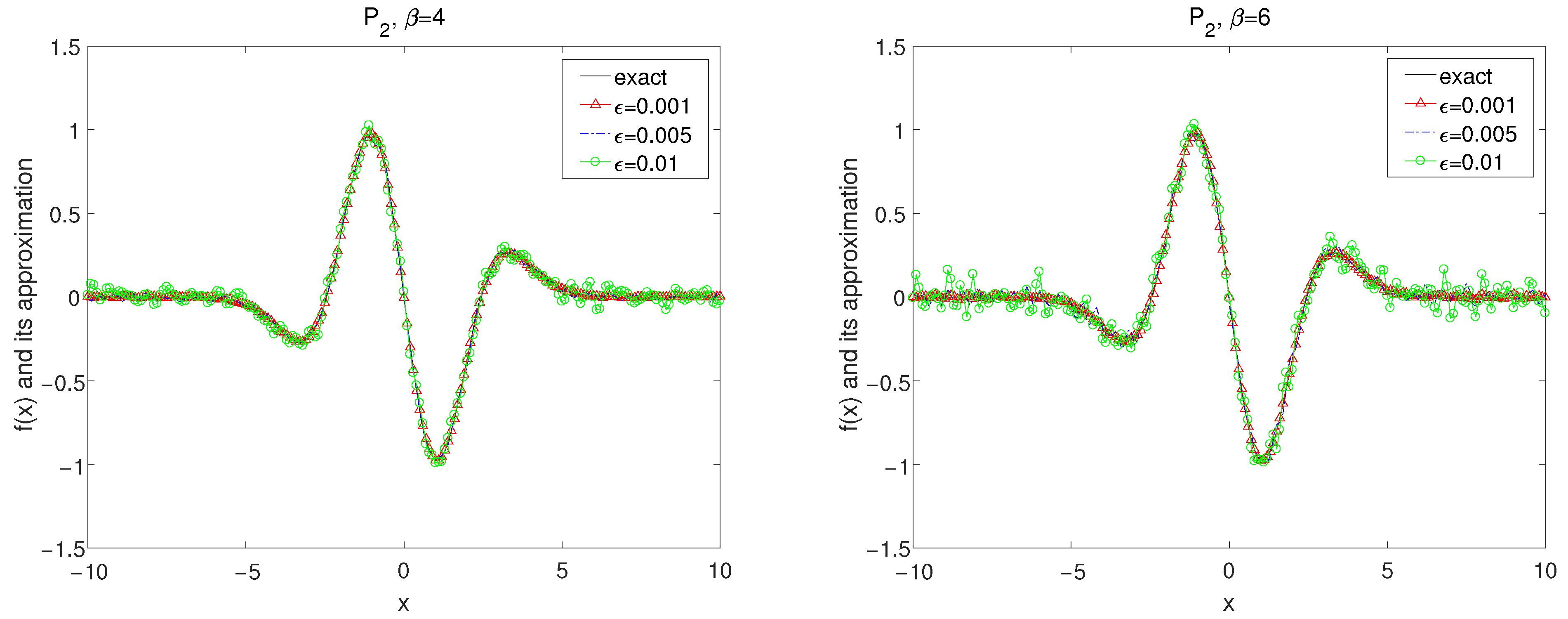
Set $f(x)=(\frac{x^3}{4}-\frac{3}{2}x)e^{-\frac{x^2}{4}}$ in the forward problem (26) and the exact data $g(x)$ is obtained by (7). It is easy to calculate by numerical method that ${\parallel f(x)\parallel }_2\approx 2.54.$ Thus, we select the a priori bound $E=3$ and $p=2$ as a source condition. The numerical results are demonstrated in Figure 1, Figure 2, Figure 3, Figure 4, Figure 5 and Figure 6.

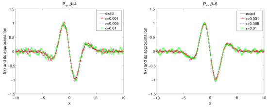
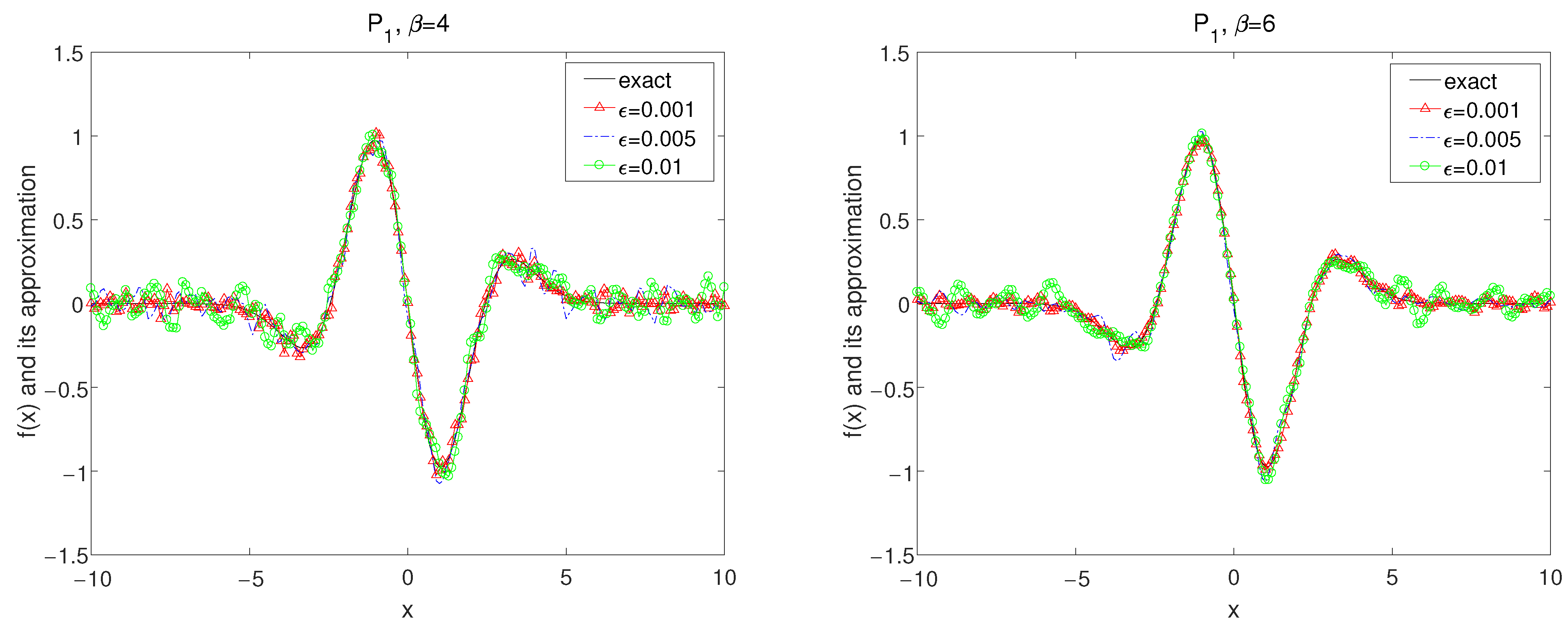
Figure 1. The exact solution and the regularized solutions with $\beta =4,6$ using kernel $P_1$ under the a priori choice rule for Example 1.

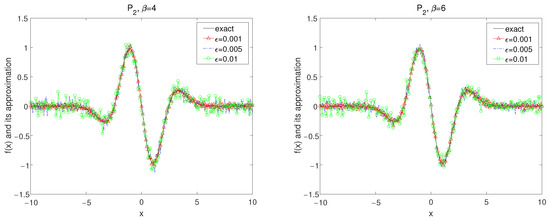
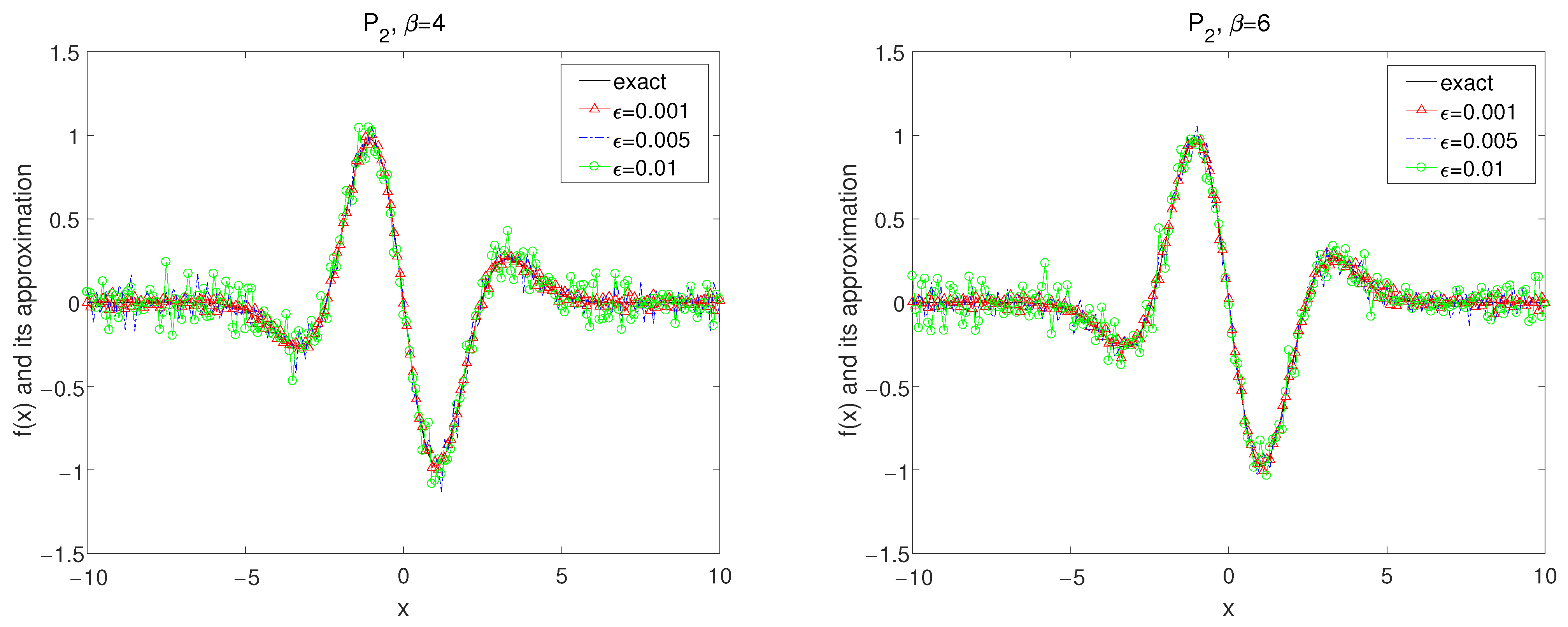
Figure 2. The exact solution and the regularized solutions with $\beta =4,6$ using kernel $P_2$ under the a priori choice rule for Example 1.

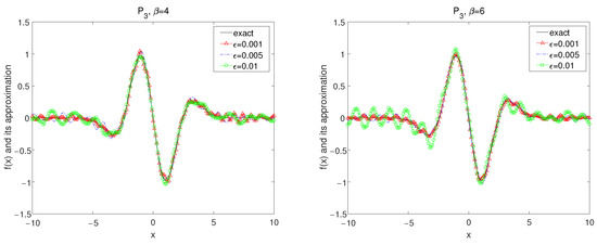
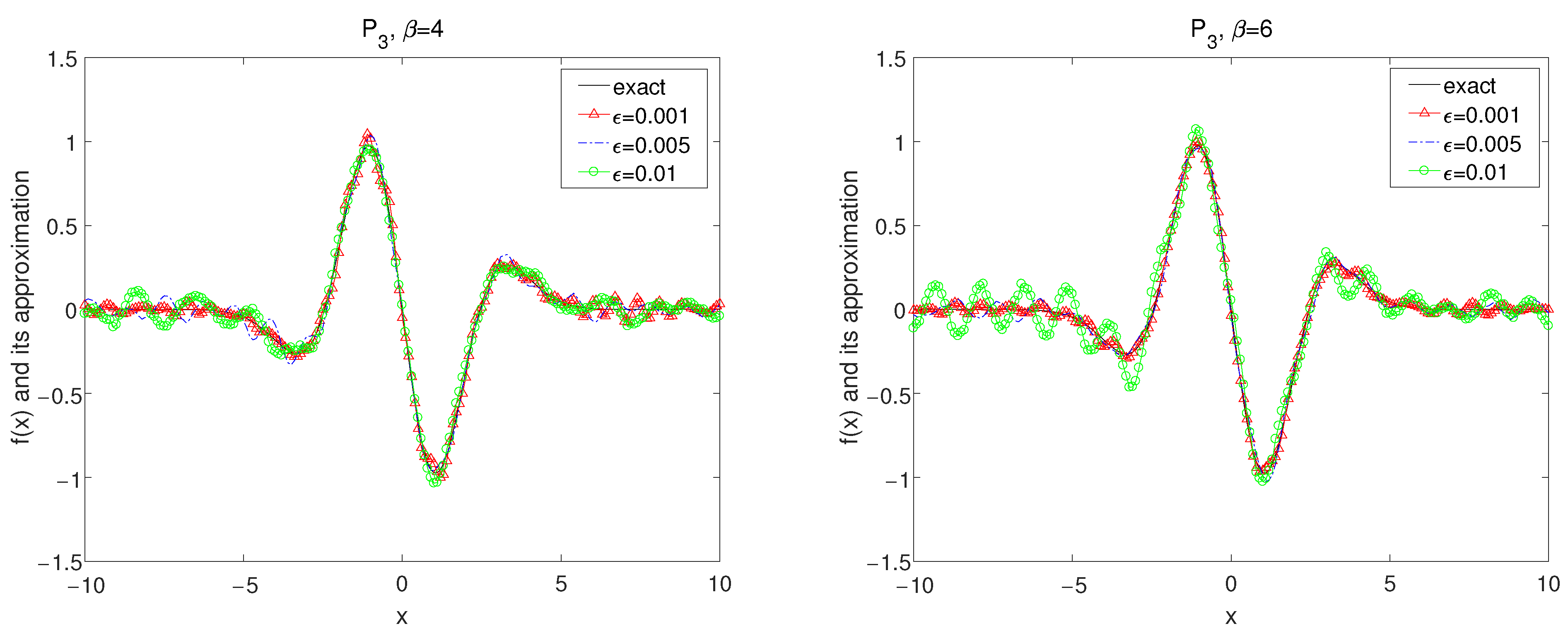
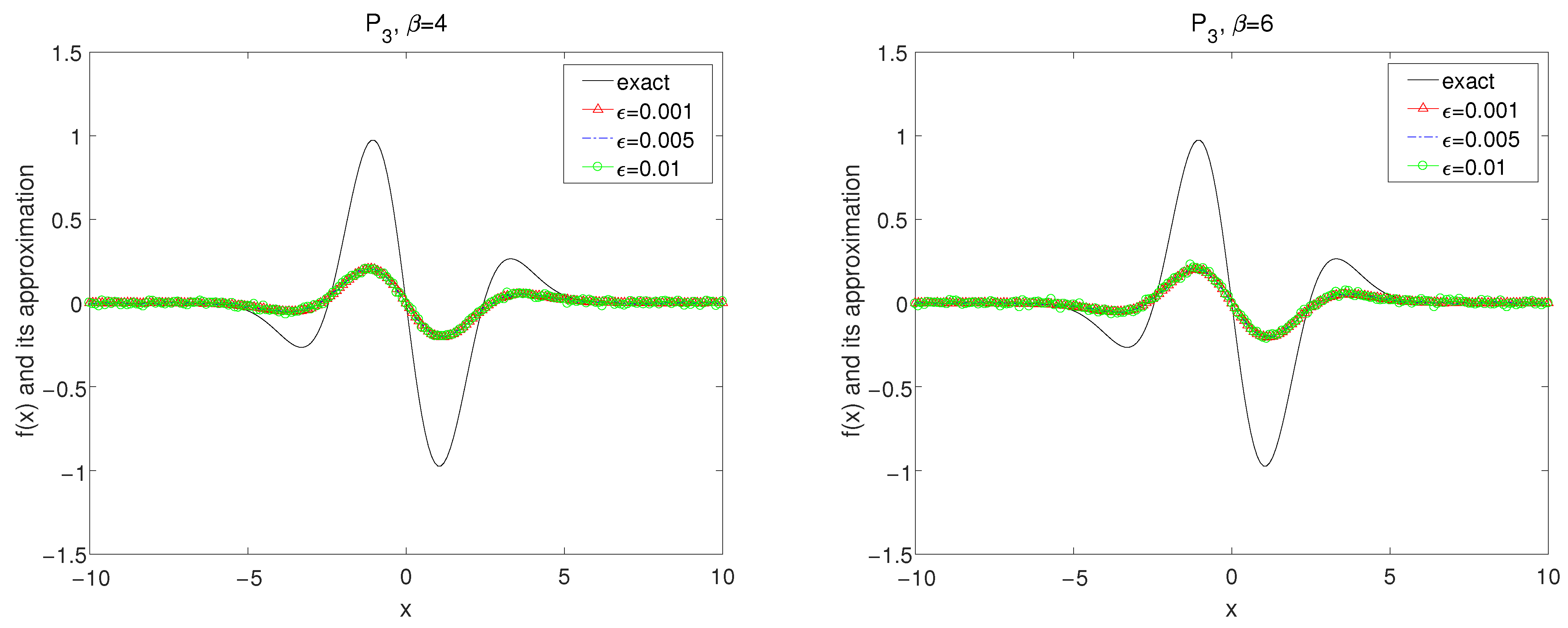
Figure 3. The exact solution and the regularized solutions with $\beta =4,6$ using kernel $P_3$ under the a priori choice rule for Example 1.

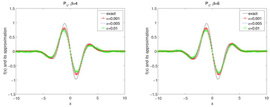
Figure 4. The exact solution and the regularized solutions with $\beta =4,6$ using kernel $P_1$ under the a posteriori choice rule for Example 1.

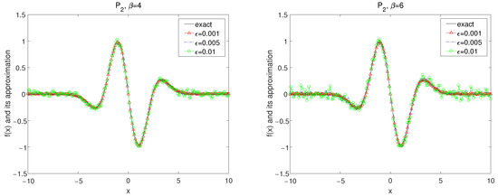
Figure 5. The exact solution and the regularized solutions with $\beta =4,6$ using kernel $P_2$ under the a posteriori choice rule for Example 1.

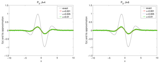
Figure 6. The exact solution and the regularized solutions with $\beta =4,6$ using kernel $P_3$ under the a posteriori choice rule for Example 1.

In Figure 1, Figure 2 and Figure 3, by using the kernel $P_1,P_2$ and $P_3$, the numerical results for convolution method under the a priori parameter choice rule for various noise levels $ϵ=0.001$, 0.005, 0.01 in case of $\beta =4,6$ are showed with $\mu =0.2102,0.2093,0.2058$ for $\beta =4,6.$

In Figure 4, Figure 5 and Figure 6, by using the kernel $P_1,P_2$ and $P_3,$ the numerical results for convolution method under the a posteriori parameter choice rule for various noise levels $ϵ=0.001$, 0.005, 0.01 in case of $\beta =4,6$ are showed with $\mu =0.5888,0.2344,0.5936$ for $\beta =4,6.$

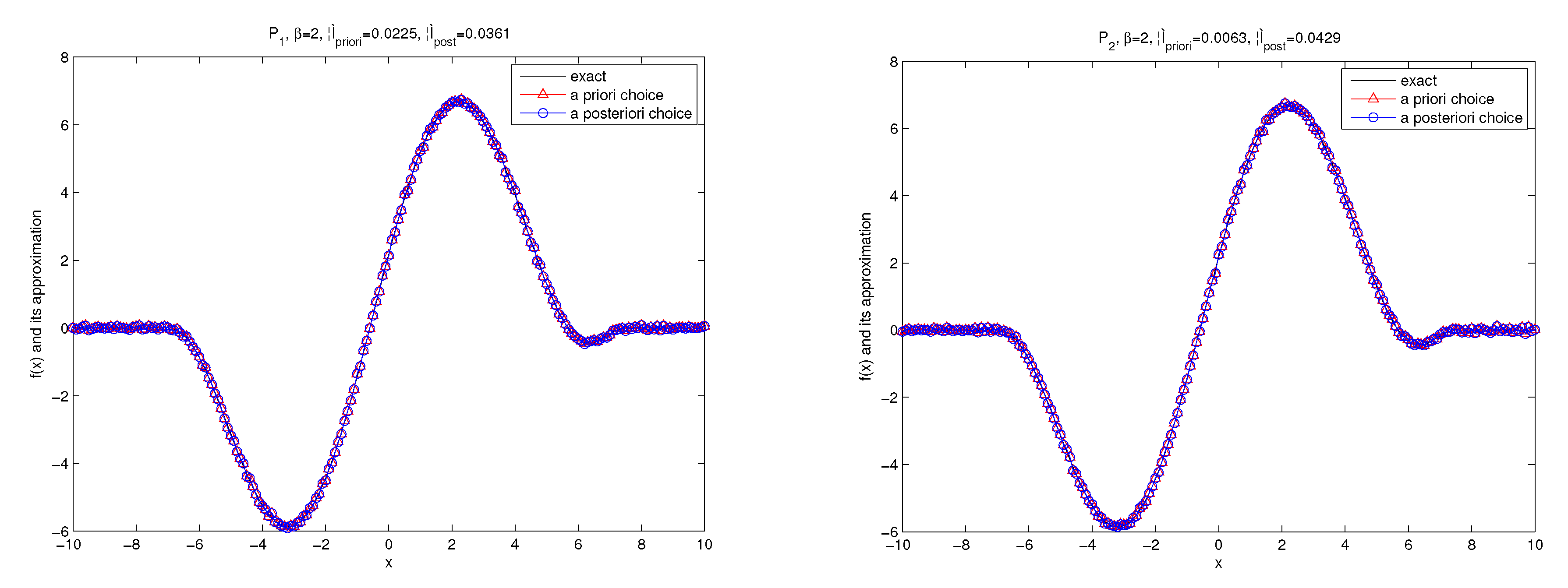
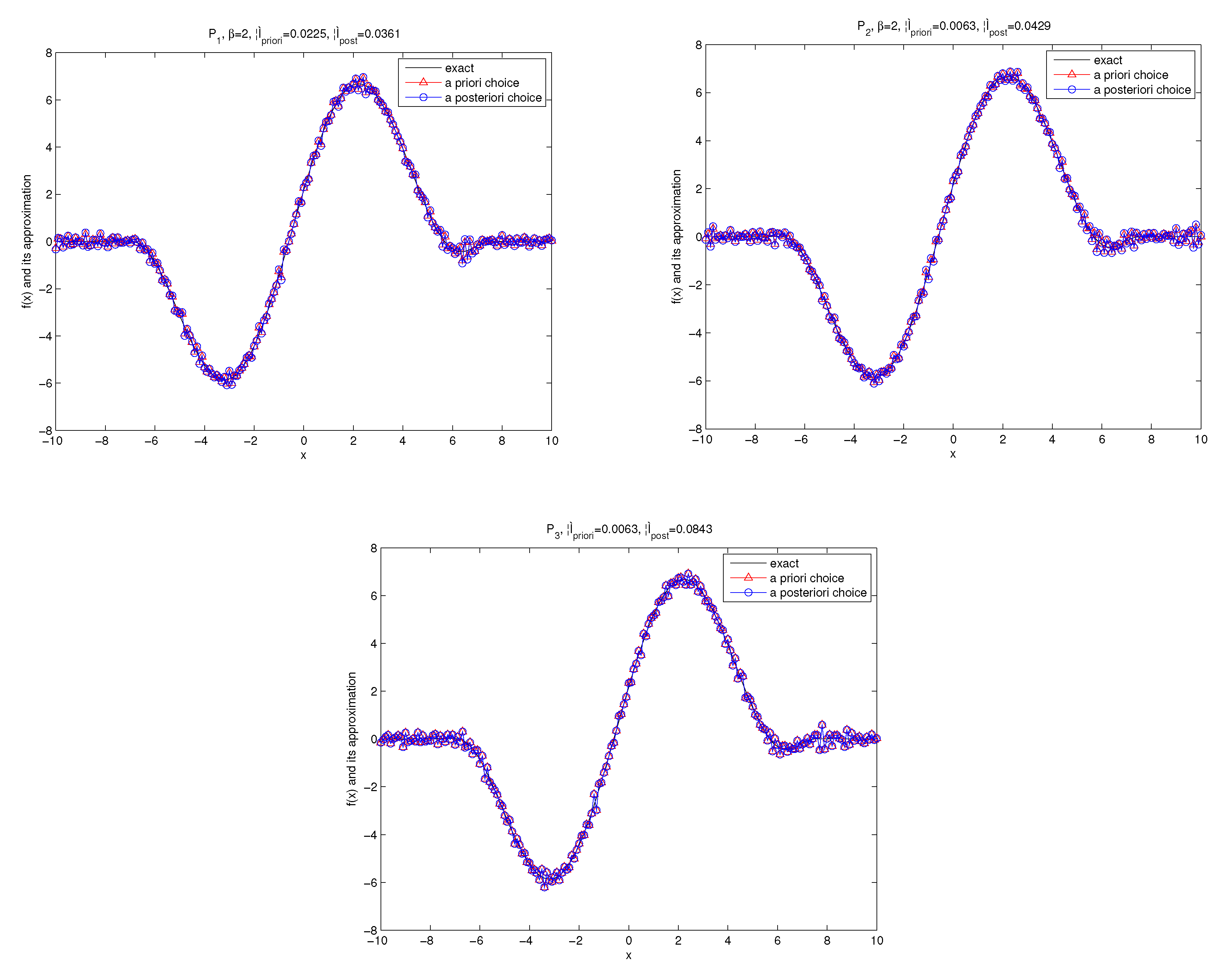
Example 2.

We test the space-fractional diffusion heat source problem.

$$\left\{\begin{array}{cc}{u}_t{=}_x{D}_{\theta }^{\alpha }u+f(x),\hfill & x\in \mathbb{R},t>0,\hfill \\ u(x,0)=0,\hfill & x\in \mathbb{R},\hfill \\ u(x,T)=g(x),\hfill & x\in \mathbb{R}.\hfill \end{array}\right.$$

(27)

In our experiments, we take $\alpha =0.5,1$ and $\theta =0.1\ast min\{\alpha ,2-\alpha \}.$ Let the source be

$$f(x)\left\{\begin{array}{cc}20exp(\frac{1}{x^2/64-1})sin(x/2+0.3),\hfill & |x|<8,\hfill \\ 0,\hfill & |x|\ge 8.\hfill \end{array}\right.$$

For this example, ${\parallel f(x)\parallel }_2\approx 20.42$, so we can choose the a priori bound $E=21$. The numerical results are showed as follows.

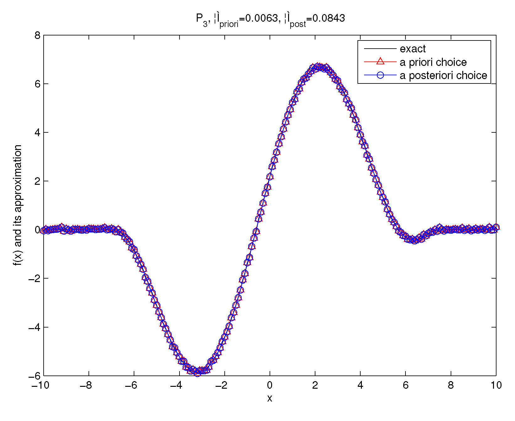
The numerical results by using the kernel $P_1(\beta =2),P_2(\beta =2)$ and the kernel $P_3$ with $ϵ=0.01$ are shown in Figure 7 and Figure 8. We know that two parameter choice rules provide accurate numerical approximations.

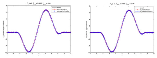
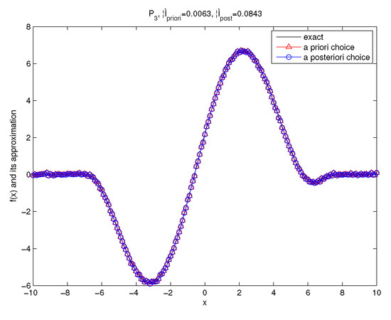
Figure 7. The exact solution and the regularized solutions of Example 2 for $\alpha =0.5$ under the a priori parameter choice and the a posteriori parameter choice.

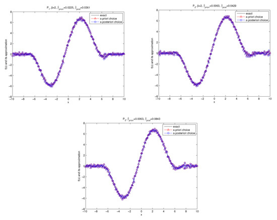
Figure 8. The exact solution and the regularized solutions of Example 2 for $\alpha =1$ under the a priori parameter choice and the a posteriori parameter choice.

6. Conclusions

In this article, a convoluting equation method is applied to determine the unknown heat source term. Furthermore, we come up with a new generalized discrepancy principle to choose the regularization parameter. The obtained results demonstrate the reliability of the proposed technique and its wider applicability to the fractional evolution equation.

References

- Cannon, J.R.; Duchateau, P. Structural identification of an unknown source term in a heat equation. Inverse Probl. 1998, 14, 535–551. [Google Scholar] [CrossRef]
- Farcas, A.; Lesnic, D. The boundary-element method for the determination of a heat source dependent on one variable. J. Eng. Math. 2006, 54, 375–388. [Google Scholar] [CrossRef]
- Li, G.S. Data compatibility and conditional stability for an inverse source problem in the heat equation. Appl. Math. Comput. 2006, 173, 566–581. [Google Scholar] [CrossRef]
- Liu, F.B. A modified genetic algorithm for solving the inverse heat transfer problem of estimating plan heat source. Int. J. Heat Mass Transf. 2008, 51, 3745–3752. [Google Scholar] [CrossRef]
- Liu, C.H. A two-stage LGSM to identify time-dependent heat source through an internal measurement of temperature. Int. J. Heat Mass Transf. 2009, 52, 1635–1642. [Google Scholar] [CrossRef]
- Ahmadabadi, M.N.; Arab, M.; Ghaini, F.M.M. The method of fundamental solutions for the inverse space-dependent heat source problem. Eng. Anal. Bound. Elem. 2009, 33, 1231–1235. [Google Scholar] [CrossRef]
- Yan, L.; Yang, F.L.; Fu, C.L. A meshless method for solving an inverse spacewise-dependent heat source problem. J. Comput. Phys. 2009, 228, 123–136. [Google Scholar] [CrossRef]
- Yamamoto, M. Conditional stability in determination of force terms of heat equations in a rectangle. Math. Comput. Model. 1993, 18, 79–88. [Google Scholar] [CrossRef]
- Hasanov, A.; Pektas, B. Identification of an unknown time-dependent heat source term from overspecified Dirichlet boundary data by conjugate gradient method. Comput. Math. Appl. 2013, 65, 42–57. [Google Scholar] [CrossRef]
- Yang, F.; Fu, C.L. A mollification regularization method for the inverse spatial-dependent heat source problem. J. Comput. Appl. Math. 2014, 255, 555–567. [Google Scholar] [CrossRef]
- Yang, F.; Fu, C.L.; Li, X.-X. A mollification regularization method for identifying the time-dependent heat source problem. J. Eng. Math. 2016, 100, 67–80. [Google Scholar] [CrossRef]
- Cannon, J.R.; Estevz, S.P. An inverse problem for the heat equation. Inverse Probl. 1986, 2, 395–403. [Google Scholar] [CrossRef]
- Choulli, M.; Yamamoto, M. Conditional stability in determining a heat source. J. Inverse Ill-Posed Probl. 2004, 12, 233–243. [Google Scholar] [CrossRef]
- Gongsheng, L.; Yamamoto, M. Stability analysis for determining a source term in a 1-D advection-dispersion equation. J. Inverse Ill-Posed Probl. 2006, 14, 147–155. [Google Scholar] [CrossRef]
- Cheng, J.; Liu, J.J. An inverse source problem for parabolic equations with local measurements. Appl. Math. Lett. 2020, 103, 106213. [Google Scholar] [CrossRef]
- Wei, H.; Chen, W.; Sun, H.G.; Li, X.C. A coupled method for inverse source problem of spatial fractional anomalous diffusion equations. Inverse Probl. Sci. Eng. 2010, 18, 945–956. [Google Scholar] [CrossRef]
- Mierzwiczak, M.; Kolodziej, J.A. Application of the method of fundamental solutions and radial basis functions for inverse transient heat source problem. Comput. Phys. Commun. 2010, 181, 2035–2043. [Google Scholar] [CrossRef]
- Rashedi, K.; Sarraf, A. Heat source identification of some parabolic equations based on the method of fundamental solutions. Eur. Phys. J. Plus 2018, 133, 403. [Google Scholar] [CrossRef]
- Sun, L.L.; Wei, T. Identification of the zeroth-order coefficient in a time fractional diffusion equation. Appl. Numer. Math. 2017, 111, 160–180. [Google Scholar] [CrossRef]
- Johansson, B.T.; Lesnic, D. A variational method for identifying a spacewise-dependent heat source. IMA J. Appl. Math. 2007, 72, 748–760. [Google Scholar] [CrossRef]
- Ma, Y.J.; Fu, C.L.; Zhang, Y.X. Identification of an unknown source depending on both time and space variables by a variational method. Appl. Math. Model. 2012, 36, 5080–5090. [Google Scholar] [CrossRef]
- Wang, F.; Chen, W.; Ling, L. Combinations of the method of fundamental solutions for general inverse source identification problems. Appl. Math. Comput. 2012, 219, 1173–1182. [Google Scholar] [CrossRef]
- Mierzwiczak, M.; Kolodziej, J.A. Application of the method of fundamental solutions with the Laplace transformation for the inverse transient heat source problem. J. Theor. Appl. Mech. 2012, 50, 1011–1023. [Google Scholar]
- Wang, J.G.; Zhou, Y.B.; Wei, T. Two regularization methods to identify a space-dependent source for the time-fractional diffusion equation. Appl. Numer. Math. 2013, 68, 39–57. [Google Scholar] [CrossRef]
- Dou, F.F.; Fu, C.L.; Yang, F.L. Optimal error bound and Fourier regularization for identifying an unknown source in the heat equation. J. Comput. Appl. Math. 2009, 230, 728–737. [Google Scholar] [CrossRef] [Green Version]
- Dou, F.F.; Fu, C.L. Determining an unknown source in the heat equation by a wavelet dual least squares method. Appl. Math. Lett. 2009, 22, 661–667. [Google Scholar] [CrossRef] [Green Version]
- Xiong, X.T.; Wang, J.X. A Tikhonov-type method for solving a multidimensional inverse heat source problem in an unbounded domain. J. Comput. Appl. Math. 2012, 236, 1766–1774. [Google Scholar] [CrossRef] [Green Version]
- Thang, N.V.; Duc, N.V.; Minh, L.D.N.; Thành, N.T. Identifying an unknown source term in a time-space fractional parabolic equation. Appl. Numer. Math. 2021, 166, 313–332. [Google Scholar] [CrossRef]
- Ma, Y.K.; Prakash, P.; Deiveegan, A. Optimization method for determining the source term in fractional diffusion equation. Math. Comput. Simul. 2019, 155, 168–176. [Google Scholar] [CrossRef]
- Hussein, M.S.; Lesnic, D.; Johansson, B.T.; Hazanee, A. Identification of a multi-dimensional space-dependent heat source from boundary data. Appl. Math. Model. 2018, 54, 202–220. [Google Scholar] [CrossRef] [Green Version]
- Yang, F.; Pu, Q.; Li, X.X. The fractional Landweber method for identifying the space source term problem for time-space fractional diffusion equation. Numer. Algorithms 2021, 87, 1229–1255. [Google Scholar] [CrossRef]
- Cannon, J.R.; Van der Hoek, J. An implicit finite difference scheme for the diffusion equation subject to the specification of mass in a portion of the domain. In Numerical Solutions of Partial Differential Equations; Noye, J., Ed.; North-Holland Publishing: Amsterdam, The Netherlands, 1982; pp. 527–539. [Google Scholar]
- Li, Y.S.; Wei, T. An inverse time-dependent source problem for a timeCspace fractional diffusion equation. Appl. Math. Comput. 2018, 336, 257–271. [Google Scholar]
- Johansson, B.T.; Lesnic, D. A procedure for determining a spacewise dependent heat source and the initial temperature. Appl. Anal. 2008, 87, 265–276. [Google Scholar] [CrossRef]
- Yang, C.Y. A sequential method to estimate the strength of the heat source based on symbolic computation. Int. J. Heat Mass Transf. 1998, 41, 2245–2252. [Google Scholar] [CrossRef]
- Zheng, G.H.; Wei, T. Two regularization methods for solving a Riesz-Feller space-fractional backward diffusion problem. Inverse Probl. 2010, 26, 115017. [Google Scholar] [CrossRef]
- Shi, C.; Wang, C.; Wei, T. Convolution regularization method for backward problems of linear parabolic equations. Appl. Numer. Math. 2016, 108, 143–156. [Google Scholar] [CrossRef]
- Shi, C.; Wang, C.; Zheng, G.; Wei, T. A new a posteriori parameter choice strategy for the convolution regularization of the space-fractional backward diffusion problem. J. Comput. Appl. Math. 2015, 279, 233–248. [Google Scholar] [CrossRef]
- Mainardi, F.; Raberto, M.; Gorenflo, R.; Scalas, E. Fractional calculus and continuous-time finance II: The waiting-time distribution. Physica A 2000, 287, 468–481. [Google Scholar] [CrossRef] [Green Version]
Publisher’s Note: MDPI stays neutral with regard to jurisdictional claims in published maps and institutional affiliations. |
© 2022 by the authors. Licensee MDPI, Basel, Switzerland. This article is an open access article distributed under the terms and conditions of the Creative Commons Attribution (CC BY) license (https://creativecommons.org/licenses/by/4.0/).