Mathematical Modeling of Recursive Drug Delivery with Diffusion, Equilibrium, and Convection Coupling

Abstract

In this work, a mathematical model to describe drug delivery from polymer coatings on implants is proposed. Release predictability is useful for development and understanding of drug release mechanisms from controlled delivery systems. The proposed model considers a unidirectional recursive diffusion process which follows Fick’s second law while considering the convective phenomena from the polymer matrix to the liquid where the drug is delivered and the polymer–liquid drug distribution equilibrium. The resulting model is solved using Laplace transformation for two scenarios: (1) a constant initial condition for a single drug delivery experiment; and (2) a recursive delivery process where the liquid medium is replaced with fresh liquid after a fixed period of time, causing a stepped delivery rate. Finally, the proposed model is validated with experimental data.

1. Introduction

Polymer coatings on implants and other biomedical devices are frequently used as local drug delivery systems, which allows for in situ release in the immediate targeted tissue, optimizing the therapeutic effects. Medications can be released at controlled rates in the range of effective treatment levels, increasing their bioavailability [1]. In this sense, mathematical modeling of drug delivery and release predictability is useful in development and understanding of drug release mechanisms from controlled delivery systems. In most cases, drug diffusional mass transport is the predominant step in the control of drug release, while in others it is present in combination with polymer swelling or polymer erosion [2]. In general, it is common to use power law equations for modeling release kinetics, such as the Higuchi and Ritger–Peppas models.

The Higuchi model [3] implies various assumptions, namely, that the initial drug concentration in the polymer is higher than the drug’s solubility, that drug diffusion occurs in only one dimension (i.e., the edge effect must be negligible), that the drug particles are smaller than the polymer thickness, that matrix swelling and dissolution are negligible, that drug diffusivity is constant, and that perfect sink conditions are always attained. The Higuchi equation is provided by

$$M_t/M_{\infty }=k{t}^{1/2}$$

where the ratio $M_t/M_{\infty }$ is the fraction of drug released at time t and k is the Higuchi dissolution constant, which represents a Fickian diffusion of drugs without the matrix dissolution.

The Ritger–Peppas model [4] is a simple relationship to describe drug release from a polymeric system. This model analyzes both Fickian and non-Fickian release of drug from swelling as well as non-swelling materials; however, it is only applicable up to 60% of the drug amount released. The Ritger–Peppas release equation is provided by

$$M_t/M_{\infty }=k{t}^n$$

where the ratio $M_t/M_{\infty }$ is the fraction of drug released at time t, k is the Ritger–Peppas kinetic constant, which characterizes the drug–matrix system, and n is the exponent that indicates the drug release mechanism.

These semi-empirical models are easy to use and the established empirical rules help to explain transport mechanisms. However, they do not provide further insights into a more complex transport mechanism. Furthermore, these models might fail when specific experimental methodology or physicochemical processes are involved [5]. For this reason, it is important to develop a mathematical model to adequately study the release kinetics from polymer coatings to liquid media. In this regard, this work is about a mathematical model that describes drug delivery considering a unidirectional iterative diffusion process in Fick’s second law while considering the convective phenomena from the polymer matrix to the liquid where the drug is delivered and the polymer–liquid drug distribution equilibrium. The resulting model is solved using Laplace transformation for two scenarios: (1) a constant initial condition for a single drug delivery experiment; and (2) a recursive delivery process where the liquid medium is replaced with fresh liquid after a fixed period of time, causing a stepped delivery rate. Finally, the proposed model is validated with experimental data.

2. Model Formulation

The main goal of the following model is to understand the drug release mechanisms from controlled delivery systems. Thus, the model must be able to evaluate whether the delivery system is controlled by the diffusion of the drug in the solid matrix (usually a polymer), by convection from the polymer surface to the liquid, or by the solid–liquid drug distribution equilibrium. In particular, we are interested in the experimental configuration shown in Figure 1, where a polymer coating (solid matrix in the following) on an implant initially impregnated with the drug is immersed in a volume of liquid, $V_l$, for a fixed period of time, producing a time-varied drug concentration in the liquid bulk, $C_l\left(t\right)$, that can be measured.

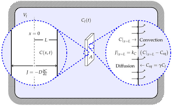
Figure 1. Scheme of the drug delivery system.

In order to model drug delivery, the following assumptions are considered:

• Drug diffusion is only in one dimension, x (i.e., the edge effect must be negligible); therefore, the concentration of the drug in the solid matrix is expressed as $C\left(x,t\right)$
• Drug particles (solute) are smaller than solid thickness
• Matrix swelling and dissolution are negligible, therefore, the length of the diffusion region, $2L$, is constant, and by symmetry the problem is analyzed in the following domain: $0\le x\le L$
• Drug diffusivity in the solid matrix, D, is constant and Fick’s law can be applied, i.e., $J=-D\partial C/\partial x$
• There exists an equilibrium between the concentration of the drug in the interface of the solid matrix and the liquid, provided by $C_{eq}=\gamma C_l$
• There is a convective rate that depends on the difference of the concentration in the solid–liquid interface, ${\left.C\right|}_{x=L}$, and the equilibrium concentration, $C_{eq}$, with the form ${\left.J\right|}_{x=L}=k_C\left({\left.C\right|}_{x=L}-C_{eq}\right)$
• The entire surface of the solid is completely submerged.

In the following sections, a model is developed for two scenarios: (1) a constant initial condition for a single drug delivery experiment; and (2) a recursive delivery process where the liquid medium is replaced with fresh liquid after a fixed period of time, causing a stepped delivery rate.

2.1. Single Drug Delivery Experiments

Consider a unidirectional diffusion of the solute in the solid matrix, described by the following partial differential equation:

$$\frac{\partial C\left(x,t\right)}{\partial t}=D\frac{{\partial }^{2}C\left(x,t\right)}{\partial x^2},\begin{array}{c}t>0\\ 0<x<L\end{array}$$

(1)

where D is the diffusivity and L is the length. The initial condition is

$$C\left(x,0\right)=C_{ini}$$

(2)

and boundary conditions are

$$\begin{array}{ccc}\hfill \frac{\partial C\left(0,t\right)}{\partial x}& =& 0\hfill \end{array}$$

(3)

$$\begin{array}{ccc}\hfill -D\frac{\partial C\left(L,t\right)}{\partial x}& =& k_C\left[C\left(L,t\right)-\gamma C_l\left(t\right)\right]\hfill \end{array}$$

(4)

where $C_l\left(t\right)$ is the solute concentration in the liquid, $k_C$ is the mass transfer coefficient in the liquid, and $\gamma$ is the solute solid–liquid partition coefficient associated with the equilibrium. Condition (2) indicates that the initial concentration in the solid matrix is homogeneous and equal to $C_{ini}$. Condition (3) appears due to the symmetry of diffusion in the middle of the solid, while condition (4) represents the solid–liquid interface. The accumulation of the solute in the liquid can be easily obtained from the mass balance,

$$V_l\frac{d{C}_l\left(t\right)}{dt}=A{k}_C\left[C\left(L,t\right)-\gamma C_l\left(t\right)\right]$$

(5)

where A is the area of mass transport and $V_l$ is the volume of the liquid. The total solute mass in the solid matrix and the liquid is constant and equal to

$$m_{ini}=A{\int }_0^{L}C\left(x,t\right)dx+V_l{C}_l\left(t\right)$$

(6)

where $m_{ini}$ is the initial solute mass in the solid matrix and, assuming that initially the solute concentration in the liquid is zero $C_l\left(0\right)=0$, it is equivalent to

$$m_{ini}=A{\int }_0^{L}C\left(x,0\right)dx=AL{C}_{ini}.$$

(7)

Notice that the time derivative of Equation (6) provides

$$V_l\frac{d{C}_l\left(t\right)}{dt}=-A{\int }_0^L\frac{\partial C\left(x,t\right)}{\partial t}dx$$

and considering Equation (1) and boundary condition (3), the previous equation becomes

$$V_l\frac{d{C}_l\left(t\right)}{dt}=-DA\frac{\partial C\left(L,t\right)}{\partial x},$$

which agrees with the substitution of Equation (4) in Equation (5). The mass of the solute in the liquid is therefore

$$C_l\left(t\right)=\frac{m_{ini}-m\left(t\right)}{V_l}=A\frac{L{C}_{ini}-{\int }_0^{L}C\left(x,t\right)dx}{V_l}$$

(8)

where $m\left(t\right)=A{\int }_0^{L}C\left(x,t\right)dx$ is the total mass of the solute in the solid matrix. Finally, replacing Equation (8) in boundary condition (4), it follows that

$$\frac{L}{\mathrm{Sh}}\frac{\partial C\left(L,t\right)}{\partial x}+C\left(L,t\right)=\beta \left[\frac{m_{ini}}{AL}-\frac{1}{L}{\int }_0^{L}C\left(x,t\right)dx\right]$$

(9)

where $\beta =\gamma \frac{AL}{V_l}$ and $\mathrm{Sh}=\frac{k_C}{D/L}$ are the Sherwood number, which represents the ratio of convective mass transfer to the rate of diffusive mass transport.

2.2. Recursive Delivery Experiment

Now, let us consider an iterative process where for each fixed period of time $\delta$ the liquid is replaced by fresh liquid without solute. Then, the iterative process can be modeled by the diffusion equation,

$$\frac{\partial C_k\left(x,t\right)}{\partial t}=D\frac{{\partial }^2{C}_k\left(x,t\right)}{\partial x^2},\begin{array}{c}k\delta <t\le \left(k+1\right)\delta \\ 0<x<L\end{array}$$

(10)

with an initial condition that depends on the concentration of the previous iteration:

$$C_k\left(x,k\delta \right)=C_{k-1}\left(x,k\delta \right)$$

(11)

and the following boundary conditions:

$$\begin{array}{ccc}\hfill \frac{\partial C_k\left(0,t\right)}{\partial x}& =& 0\hfill \end{array}$$

(12)

$$\begin{array}{ccc}\hfill \frac{L}{\mathrm{Sh}}\frac{\partial C\left(L,t\right)}{\partial x}+C_k\left(L,t\right)& =& \beta \left[\frac{m_{0,k}}{AL}-\frac{{\int }_0^L{C}_k\left(x,t\right)dx}{L}\right]k\delta <t\le \left(k+1\right)\delta \hfill \end{array}$$

(13)

where $k=1,2,3,\dots$ and the initial mass of the solute in the solid at iteration k depends on the final concentration of iteration $k-1$, i.e.,

$$m_{0,k}=A{\int }_0^L{C}_{k-1}\left(x,k\delta \right)dx.$$

To analyze the iterative behavior, it is proposed that a shift in time ${\tau }_k=t-k\delta$ be defined in such a way that the previous model becomes

$$\frac{\partial C_k\left(x,{\tau }_k\right)}{\partial {\tau }_k}=D\frac{{\partial }^2{C}_k\left(x,{\tau }_k\right)}{\partial x^2},\begin{array}{c}{\tau }_k>0\\ 0<x<L\end{array}$$

(14)

$$C_k\left(x,0\right)={\left[C_{k-1}\left(x,{\tau }_{k-1}\right)\right]}_{{\tau }_{k-1}=\delta }$$

(15)

$$\begin{array}{ccc}\hfill \frac{\partial C_k\left(0,{\tau }_k\right)}{\partial x}& =& 0\hfill \end{array}$$

(16)

$$\begin{array}{ccc}\hfill \frac{L}{\mathrm{Sh}}\frac{\partial C_k\left(L,{\tau }_k\right)}{\partial x}+C_k\left(L,{\tau }_k\right)& =& \beta \left[\frac{m_{0,k}}{AL}-\frac{{\int }_0^L{C}_k\left(x,{\tau }_k\right)dx}{L}\right]\hfill \end{array}$$

(17)

for $k=1,2,3,\dots$. Then, the analytical solution of the models for the two scenarios is presented in the following section using Laplace transformation [6].

3. Analytical Solutions

3.1. Single Drug Delivery Experiment

To solve the problem described by Equations (1)–(3) and (9), let us define the Laplace transformation:

$$\mathcal{L}\left\{C\left(x,t\right)\right\}={\int }_0^{\infty }C\left(x,t\right)e^{-st}dt=\widehat{C}\left(x,s\right)$$

(18)

therefore, the Laplace transformation of Equation (1) is

$$s\widehat{C}\left(x,s\right)-C_{ini}=D\frac{d^2\widehat{C}\left(x,s\right)}{d{x}^2},0<x<L$$

(19)

while the Laplace transformations of the boundary conditions (Equations (3) and (9)) are

$$\begin{array}{ccc}\hfill \frac{d\widehat{C}\left(0,s\right)}{dx}& =& 0,\hfill \end{array}$$

(20)

$$\begin{array}{ccc}\hfill \frac{L}{\mathrm{Sh}}\frac{d\widehat{C}\left(L,s\right)}{dx}+\widehat{C}\left(L,s\right)& =& \beta \left[\frac{\frac{m_{ini}}{AL}}{s}-\frac{1}{L}{\int }_0^L\widehat{C}\left(x,s\right)dx\right].\hfill \end{array}$$

(21)

The solution of Equation (19) together with Conditions (20) and (21) is

$$\widehat{C}\left(x,s\right)=\frac{C_{ini}}{s}\left[1-\frac{\rho cosh\left(x\sqrt{\frac{s}{D}}\right)}{cosh\left(L\sqrt{\frac{s}{D}}\right)+\frac{1}{L}\sqrt{\frac{D}{s}}\left(\frac{L^{2}s}{D\mathrm{Sh}}+\beta \right)sinh\left(L\sqrt{\frac{s}{D}}\right)}\right]$$

(22)

where $\rho =1+\beta \left(1-\frac{m_{ini}}{C_{ini}AL}\right)$. Notice that, for this particular case $\rho =1$, because $m_{ini}=AL{C}_{ini}$; however, here, we use $\rho$, as the general solution for $\rho \ne 1$ is used for the recursive problem analyzed latter.

The concentration profile can be obtained by applying the inverse Laplace transformation to Equation (22). The inverse of the first term can be obtained with the formula ${\mathcal{L}}^{-1}\left\{\frac{1}{s}\right\}=1$, while for the second term a more elaborated procedure is required.

We define

$$p\left(s\right)=cosh\left(\frac{x}{L}\sqrt{\frac{L^{2}s}{D}}\right)$$

and

$$q\left(s\right)=cosh\sqrt{\frac{L^{2}s}{D}}+\sqrt{\frac{D}{L^{2}s}}\left(\beta +\frac{1}{\mathrm{Sh}}\frac{L^{2}s}{D}\right)sinh\sqrt{\frac{L^{2}s}{D}}.$$

where for $s_n=-D{\left(\frac{{\alpha }_n}{L}\right)}^2$, it holds that

$$q\left(s_n\right)=cos\left({\alpha }_n\right)+\left(\frac{\beta }{{\alpha }_n}-\frac{{\alpha }_n}{\mathrm{Sh}}\right)sin\left({\alpha }_n\right).$$

Thus, the values of ${\alpha }_n$ at which $q\left(s_n\right)=0$ are provided by the characteristic equation

$$tan\left({\alpha }_n\right)=\frac{{\alpha }_n}{\frac{{\alpha }_n^2}{\mathrm{Sh}}-\beta }.$$

(23)

according to the following formula:

$${\mathcal{L}}^{-1}\left\{\frac{p\left(s\right)}{q\left(s\right)}\right\}=\sum _{n=1}^{\infty }\frac{p\left(s_n\right)}{q^{\prime }\left(s_n\right)}exp\left(s_{n}t\right)$$

(24)

where $p\left(s\right)$ and $q\left(s\right)$ are infinite series of s, $q^{\prime }\left(s\right)$ is the derivative of $q\left(s\right)$ with respect to s, and $s_n$ are the infinite values of s satisfying the equation $q\left(s\right)=0$; thus, the following inverse transformation is obtained

$${\mathcal{L}}^{-1}\left\{\frac{p\left(s\right)}{q\left(s\right)}\right\}=\frac{2D}{L^2}\sum _{n=1}^{\infty }\frac{{\alpha }_n^{3}cos\left({\alpha }_n\frac{x}{L}\right)exp\left(-D{\left(\frac{{\alpha }_n}{L}\right)}^{2}t\right)}{\left[\beta +{\alpha }_n^2\left(1+\frac{1}{\mathrm{Sh}}\right)+{\left(\beta -\frac{{\alpha }_n^2}{\mathrm{Sh}}\right)}^2\right]sin\left({\alpha }_n\right)}.$$

Finally, for any arbitrary function $f\left(s\right)=\mathcal{L}\left\{f\left(t\right)\right\}$, the following inverse Laplace transformation holds: ${\mathcal{L}}^{-1}\left\{\frac{f\left(s\right)}{s}\right\}={\int }_0^{t}F\left(\tau \right)d\tau$; then,

$${\mathcal{L}}^{-1}\left\{\frac{1}{s}·\frac{p\left(s\right)}{q\left(s\right)}\right\}=2\sum _{n=1}^{\infty }\frac{cos\left({\alpha }_n\frac{x}{L}\right)\left[1-exp\left(-D{\left(\frac{{\alpha }_n}{L}\right)}^{2}t\right)\right]}{\left[{\alpha }_n\left(1+\frac{1-2\beta +{\alpha }_n^2/\mathrm{Sh}}{\mathrm{Sh}}\right)+\frac{\left(1+\beta \right)\beta }{{\alpha }_n}\right]sin\left({\alpha }_n\right)}$$

and the concentration becomes the following Fourier series [7]:

$$C\left(x,t\right)=C_{ini}\left[1-2\rho \sum _{n=1}^{\infty }\frac{cos\left({\alpha }_n\frac{x}{L}\right)\left[1-exp\left(-D{\left(\frac{{\alpha }_n}{L}\right)}^{2}t\right)\right]}{\left[{\alpha }_n\left(1+\frac{1-2\beta +{\alpha }_n^2/\mathrm{Sh}}{\mathrm{Sh}}\right)+\frac{\left(1+\beta \right)\beta }{{\alpha }_n}\right]sin\left({\alpha }_n\right)}\right].$$

(25)

The relationship between the mass at any time and the initial mass of solute in the solid matrix is

$$\frac{m\left(t\right)}{m_{ini}}=\frac{1}{L}{\int }_0^L\frac{C\left(x,t\right)}{C_{ini}}dx$$

and considering the solution, this integral is

$$\frac{{\int }_0^L\frac{C\left(x,t\right)}{C_{ini}}dx}{L}=1-2\rho \sum _{n=1}^{\infty }\frac{1-exp\left[-D{\left(\frac{{\alpha }_n}{L}\right)}^{2}t\right]}{{\alpha }_n^2\left(1+\frac{1-2\beta +{\alpha }_n^2/\mathrm{Sh}}{\mathrm{Sh}}\right)+\left(1+\beta \right)\beta }$$

while the amount of mass of solute that has left the solid matrix and diffused to the liquid is

$$1-\frac{m\left(t\right)}{m_{ini}}=2\rho \sum _{n=1}^{\infty }\frac{1-exp\left[-D{\left(\frac{{\alpha }_n}{L}\right)}^{2}t\right]}{{\alpha }_n^2\left(1+\frac{1-2\beta +{\alpha }_n^2/\mathrm{Sh}}{\mathrm{Sh}}\right)+\left(1+\beta \right)\beta }$$

At steady state, the concentration in the solid matrix does not depend on time; thus, $C\left(x,t\right)$ becomes $C^{*}\left(x\right)$. Therefore, Equation (1) reduces to

$$D\frac{d^2{C}^{*}\left(x\right)}{d{x}^2}=0$$

(26)

while conditions (3) and (4) become

$$\begin{array}{ccc}\hfill \frac{d{C}^{*}\left(0\right)}{dx}& =& 0\hfill \end{array}$$

(27)

$$\begin{array}{ccc}\hfill \frac{L}{\mathrm{Sh}}\frac{d{C}^{*}\left(L\right)}{dx}+C^{*}\left(L\right)& =& \beta \left[\frac{m_{ini}}{AL}-\frac{1}{L}{\int }_0^L{C}^{*}\left(x\right)dx\right]\hfill \end{array}$$

(28)

The solution of Equation (26) together with the boundary conditions (27) and (28) is

$$C^{*}\left(x\right)=\frac{\beta }{1+\beta }\frac{m_{ini}}{AL}=\gamma C_{l,\infty }$$

(29)

where $C_{l,\infty }$ is the steady state concentration of the solute in the liquid. Notice that the steady state concentration profile of the solute in the solid matrix is constant.

Now, considering the transient solution (25) and the solution at steady state (29), given that $C^{*}\left(x\right)={lim}_{t\to \infty }C\left(x,t\right)$ it is straightforward to verify that the following Fourier series can be expressed as

$$2\sum _{n=1}^{\infty }\frac{cos\left({\alpha }_n\frac{x}{L}\right)}{\left[{\alpha }_n\left(1+\frac{1-2\beta +{\alpha }_n^2/\mathrm{Sh}}{\mathrm{Sh}}\right)+\frac{\left(1+\beta \right)\beta }{{\alpha }_n}\right]sin\left({\alpha }_n\right)}=\frac{1}{1+\beta }$$

(30)

and solution (25) is equivalent to

$$C\left(x,t\right)=\frac{\beta }{1+\beta }\frac{m_{ini}}{AL}+2\rho C_{ini}\sum _{n=1}^{\infty }\frac{cos\left({\alpha }_n\frac{x}{L}\right)exp\left[-D{\left(\frac{{\alpha }_n}{L}\right)}^{2}t\right]}{\left[{\alpha }_n\left(1+\frac{1-2\beta +{\alpha }_n^2/\mathrm{Sh}}{\mathrm{Sh}}\right)+\frac{\left(1+\beta \right)\beta }{{\alpha }_n}\right]sin\left({\alpha }_n\right)}.$$

(31)

The integral of this concentration is

$$\frac{m\left(t\right)}{m_{ini}}=\frac{1}{L}{\int }_0^L\frac{C\left(x,t\right)}{C_0}dx=\frac{\beta }{1+\beta }\frac{m_{ini}}{AL{C}_{ini}}+2\rho \sum _{n=1}^{\infty }\frac{exp\left[-D{\left(\frac{{\alpha }_n}{L}\right)}^{2}t\right]}{{\alpha }_n^2\left(1+\frac{1-2\beta +{\alpha }_n^2/\mathrm{Sh}}{\mathrm{Sh}}\right)+\left(1+\beta \right)\beta },$$

and the mass of the solute in the liquid is

$$\frac{m_l\left(t\right)}{m_{ini}}:=1-\frac{m\left(t\right)}{m_{ini}}=\rho \left[\frac{1}{1+\beta }-2\sum _{n=1}^{\infty }\frac{exp\left[-D{\left(\frac{{\alpha }_n}{L}\right)}^{2}t\right]}{{\alpha }_n^2\left(1+\frac{1-2\beta +{\alpha }_n^2/\mathrm{Sh}}{\mathrm{Sh}}\right)+\left(1+\beta \right)\beta }\right].$$

(32)

3.2. Recursive Delivery Experiment

In order to solve this problem, we first state that

$$C_k\left(x,{\tau }_k\right)=C_{k-1}\left(x,{\tau }_{k-1}+\delta \right)+W_k\left(x,{\tau }_k\right),$$

(33)

where $W_k\left(x,{\tau }_k\right)$ is an auxiliary variable and $C_{k-1}\left(x,{\tau }_{k-1}+\delta \right)$ is the solution at the previous iteration. Therefore, the substitution of Equation (33) in Equation (14) and conditions (15)–(17) produces the following problem for $W_k\left(x,{\tau }_k\right)$:

$$\frac{\partial W_k\left(x,{\tau }_k\right)}{\partial {\tau }_k}=D\frac{{\partial }^2{W}_k\left(x,{\tau }_k\right)}{\partial x^2},\begin{array}{c}{\tau }_k>0\\ 0<x<L\end{array}$$

(34)

$$W_k\left(x,0\right)=0$$

(35)

$$\begin{array}{ccc}\hfill \frac{\partial W_k\left(0,{\tau }_k\right)}{\partial x}& =& 0\hfill \end{array}$$

(36)

$$\begin{array}{ccc}\hfill \frac{L}{\mathrm{Sh}}\frac{\partial W_k\left(L,{\tau }_k\right)}{\partial x}+W_k\left(L,{\tau }_k\right)+\beta \frac{{\int }_0^L{W}_k\left(x,{\tau }_k\right)dx}{L}& =& \beta \left(\frac{m_{0,k}-m_{0,k-1}}{AL}\right)\hfill \end{array}$$

(37)

where

$$\begin{array}{ccc}\hfill m_{0,k}& =& A{\int }_0^L{\left[C_{k-1}\left(x,{\tau }_{k-1}\right)\right]}_{{\tau }_{k-1}=\delta }dx,\hfill \\ \hfill m_{0,k-1}& =& A{\int }_0^L{\left[C_{k-1}\left(x,{\tau }_{k-1}\right)\right]}_{{\tau }_{k-1}=0}dx.\hfill \end{array}$$

Notice that Equations (34)–(37) are analogue to Equations (1)–(3) and (9) with $C_{ini}=0$ and $m_{ini}=m_{0,k}-m_{0,k-1}$; therefore, the solution is

$$W_k\left(x,{\tau }_k\right)=2\beta \left(\frac{m_{0,k}-m_{0,k-1}}{AL}\right)\sum _{n=1}^{\infty }\frac{cos\left({\alpha }_n\frac{x}{L}\right)\left[1-exp\left(-D{\left(\frac{{\alpha }_n}{L}\right)}^2{\tau }_k\right)\right]}{\left[{\alpha }_n\left(1+\frac{1-2\beta +{\alpha }_n^2/\mathrm{Sh}}{\mathrm{Sh}}\right)+\frac{\left(1+\beta \right)\beta }{{\alpha }_n}\right]sin\left({\alpha }_n\right)}$$

while considering the identity in (30), this function becomes

$$W_k\left(x,{\tau }_k\right)=\beta \left(\frac{m_{0,k}-m_{0,k-1}}{AL}\right)\left[1-W_0\left(x,{\tau }_k\right)\right]$$

where

$$W_0\left(x,t\right)=\frac{\beta }{1+\beta }+2\sum _{n=1}^{\infty }\frac{cos\left({\alpha }_n\frac{x}{L}\right)exp\left[-D{\left(\frac{{\alpha }_n}{L}\right)}^{2}t\right]}{\left[{\alpha }_n\left(1+\frac{1-2\beta +{\alpha }_n^2/\mathrm{Sh}}{\mathrm{Sh}}\right)+\frac{\left(1+\beta \right)\beta }{{\alpha }_n}\right]sin\left({\alpha }_n\right)}.$$

The concentration provided in Equation (33) becomes

$$C_k\left(x,{\tau }_k\right)=C_{k-1}\left(x,{\tau }_{k-1}+\delta \right)+\beta \left(\frac{m_{0,k}-m_{0,k-1}}{AL}\right)\left[1-W_0\left(x,{\tau }_k\right)\right],$$

which in terms of the original time variable is

$$C_k\left(x,t\right)=C_{k-1}\left(x,t\right)+\beta \left(\frac{m_{0,k}-m_{0,k-1}}{AL}\right)\left[1-W_0\left(x,t-k\delta \right)\right],\begin{array}{c}k\delta <t\le \left(k+1\right)\delta \\ 0<x<L\end{array}.$$

(38)

Notice that for $k=0$, the solution is obtained through Equations (25) or (31)

$$C_0\left(x,t\right)=C_{ini}{W}_0\left(x,t\right),\begin{array}{c}0<t\le \delta \\ 0<x<L\end{array};$$

for $k=1$, it holds that

$$C_1\left(x,t\right)=C_{ini}{W}_0\left(x,t\right)+\beta \left(\frac{m_{0,1}}{AL}-C_{ini}\right)\left[1-W_0\left(x,t-\delta \right)\right],\begin{array}{c}\delta <t\le 2\delta \\ 0<x<L\end{array},$$

while for $k=2$,

$$\begin{array}{ccc}\hfill C_2\left(x,t\right)& =& C_{ini}{W}_0\left(x,t\right)+\beta \left(\frac{m_{0,1}}{AL}-C_{ini}\right)\left[1-W_0\left(x,t-\delta \right)\right]\hfill \\ & & +\beta \left(\frac{m_{0,2}-m_{0,1}}{AL}\right)\left[1-W_0\left(x,t-2\delta \right)\right],\begin{array}{c}2\delta <t\le 3\delta \\ 0<x<L\end{array}.\hfill \end{array}$$

and in general,

$$\frac{C_k\left(x,t\right)}{C_{ini}}=W_0\left(x,t\right)+\beta \sum _{i=1}^k\left(\frac{m_{0,i}}{m_{0,0}}-\frac{m_{0,i-1}}{m_{0,0}}\right)\left[1-W_0\left(x,t-i\delta \right)\right],\begin{array}{c}k\delta <t\le \left(k+1\right)\delta \\ 0<x<L\end{array}$$

(39)

where $m_{0,0}=AL{C}_{ini}=m_{ini}$.

The total fraction of solute mass inside the solid matrix with respect to the initial solute mass at each instant is

$$\frac{m_k\left(t\right)}{m_{0,0}}=\frac{A{\int }_0^L{C}_k\left(x,t\right)dx}{m_{0,0}}=M_0\left(t\right)+\beta \sum _{i=1}^k\left(\frac{m_{0,i}}{m_{0,0}}-\frac{m_{0,i-1}}{m_{0,0}}\right)\left[1-M_0\left(t-i\delta \right)\right]$$

where

$$M_0\left(t\right)=\frac{1}{L}{\int }_0^L{W}_0\left(x,t\right)dx=\frac{\beta }{1+\beta }+2\sum _{n=1}^{\infty }\frac{exp\left[-D{\left(\frac{{\alpha }_n}{L}\right)}^{2}t\right]}{{\alpha }_n^2\left(1+\frac{1-2\beta +{\alpha }_n^2/\mathrm{Sh}}{\mathrm{Sh}}\right)+\left(1+\beta \right)\beta }$$

therefore,

$$\frac{m_{0,1}}{m_{0,0}}=M_0\left(\delta \right)$$

and

$$\frac{m_{0,k}}{m_{0,0}}=\frac{m_{k-1}\left(k\delta \right)}{m_{0,0}}=M_0\left(k\delta \right)+\beta \sum _{i=1}^{k-1}\left(\frac{m_{0,i}}{m_{0,0}}-\frac{m_{0,i-1}}{m_{0,0}}\right)\left[1-M_0\left(\left(k-i\right)\delta \right)\right],k=2,3,\dots$$

Finally, the mass of the solute that has been delivered from the solid matrix is

$$\frac{m_{l,k}\left(t\right)}{m_{0,0}}:=1-\frac{m_k\left(t\right)}{m_{0,0}}=1-M_0\left(t\right)-\beta \sum _{i=1}^k\left(\frac{m_{0,i}}{m_{0,0}}-\frac{m_{0,i-1}}{m_{0,0}}\right)\left[1-M_0\left(t-i\delta \right)\right].$$

(40)

4. Case Study

4.1. Materials and Methods

Surface sections ($1\times 1{\mathrm{cm}}^2$) from a roughness breast implant purchased from Mentor® brand (USA) were polymerized with (2-Hydroxypropyl)-b-cyclodextrin and citric acid according to the protocol of [8]. Samples were loaded with a concentrated solution of Rose Bengal (RB) stain for 12 h. The RB release profile, $C_l\left(t\right)$, was obtained as a mean of triplicate experiments. Loaded samples were placed into vials filled with phosphate-buffered saline (PBS) at 37 °C in a horizontal shaker (100 rpm) (NB-2005LN Biotek, Winooski, VT, USA). In order to maintain perfect sink conditions, the PBS medium of the samples was changed every 24 h, for ten times in total. The RB content in the withdrawn bulk PBS was analyzed by UV-spectrophotometry (Evolution 220 model, Thermo Scientific, Waltham, MA, USA) at 545 nm [9]. Reactive chemicals were obtained from Sigma-Aldrich® (St. Louis, MO, USA).

4.2. Model Prediction

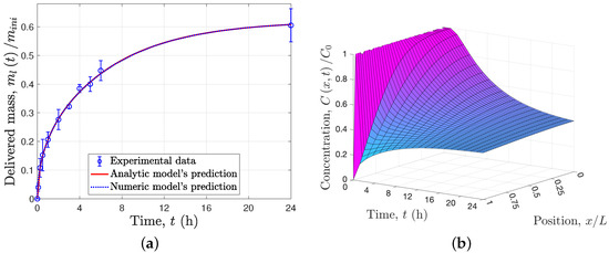
Figure 2a shows the RB release profile for the first 24 h of the experiment as $m_l\left(t\right)/m_{ini}$ vs. t. As a first approach, these experimental data were used to estimate the three parameters of the model presented in Section 2.1 $\left(D,\beta ,\mathrm{Sh}\right)$, with a least-squares method using a derivative-free algorithm [10] to minimize the sum of the squares of the error between the data and the prediction of Equation (32). As a result, a very large value was obtained for the Sherwood number, $\mathrm{Sh}=\frac{k_C}{D/L}\sim {10}^5$, suggesting that diffusion controls the interface transport for the experimental conditions; therefore, the characteristic Equation (23), the concentration profile (31), and the release profile (32) can be simplified to $tan\left({\alpha }_n\right)=-{\alpha }_n/\beta$:

$$\frac{C\left(x,t\right)}{C_{ini}}=\frac{\beta }{1+\beta }+2\sum _{n=1}^{\infty }\frac{cos\left({\alpha }_n\frac{x}{L}\right)exp\left[-D{\left(\frac{{\alpha }_n}{L}\right)}^{2}t\right]}{\left({\alpha }_n+\frac{\left(1+\beta \right)\beta }{{\alpha }_n}\right)sin\left({\alpha }_n\right)}$$

and

$$\frac{m_l\left(t\right)}{m_{ini}}=\frac{1}{1+\beta }-2\sum _{n=1}^{\infty }\frac{exp\left[-{\alpha }_n^2\frac{D}{L^2}t\right]}{{\alpha }_n^2+\left(1+\beta \right)\beta },$$

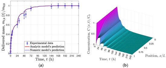
respectively. This simplified model contains only two parameters, $\left(D/L^2,\beta \right)$, the numerical values of which, $D/L^2=4.102\times {10}^{-2}$ h${}^{-1}$ and $\beta =6.095\times {10}^{-2}$, were estimated using the same least-square method [10]. Finally, the same parameters were used to predict the behavior of the recursive delivery experiment, where the PBS medium of the samples was changed every 24 h for ten days (see Figure 3a).

Figure 2. Single drug delivery. (a) Comparison of the experimental data and prediction for the delivered mass using Equation (32). (b) Prediction of the drug concentration profile in the solid matrix using Equation (31). The parameters are $D/L^2=4.102\times {10}^{-2}$ h${}^{-1}$, $\beta =6.095\times {10}^{-2}$, and ${\mathrm{Sh}}^{-1}=0$.

Figure 3. Recursive drug delivery. (a) Comparison of the experimental data and prediction for the delivered mass using Equation (40). (b) Prediction of the drug concentration profile in the solid matrix using Equation (39). The parameters are $D/L^2=4.102\times {10}^{-2}$ h${}^{-1}$, $\beta =6.095\times {10}^{-2}$, and ${\mathrm{Sh}}^{-1}=0$.

5. Discussion

The proposed models for single and recursive release experiments presented in Section 2.1 and Section 2.2, respectively, are general and allow us to clarify the predominant step in the control of drug release, This is because these models consider the drug diffusion in the solid matrix, the convective phenomenon from the solid matrix to the liquid, where the drug is delivered, and the solid–liquid drug distribution equilibrium. In particular, considering the experimental conditions of the study case presented in Section 4, diffusion dominates over convection thanks to the mixing conditions established by the horizontal shaker (with 100 rpm) in our experiments. For this reason, we was obtained ${\mathrm{Sh}}^{-1}\approx 0$, reducing the number of parameters to two, namely, $\left(D/L^2,\beta \right)$; however, convection might be relevant as well for in situ applications.

In the Higuchi model [3], the characteristic values are of the form $\left(n-\frac{1}{2}\right)\pi$, leading to the approximation $M_t/M_{\infty }=k{t}^{1/2}$. However, the assumption of solid–liquid interface equilibrium leads to the characteristic Equation (23), which depends on both Sh and $\beta$ and the characteristic values of which must be numerically computed. In particular, for ${\mathrm{Sh}}^{-1}=0$ and $\beta =6.095\times {10}^{-2}$ the first characteristic values are ${\alpha }_1\approx 0.6\pi$, ${\alpha }_2\approx 1.54\pi$, ${\alpha }_3\approx 2.524\pi$, ${\alpha }_4\approx 3.518\pi$,…, which tends towards ${\alpha }_n\to \left(n-\frac{1}{2}\right)\pi$ as n increases (see Figure 4). The deviation from $\left(n-\frac{1}{2}\right)\pi$ of the first characteristic values produces a response that is non necessarily proportional to $t^{1/2}$, as in the Higuchi model [3].

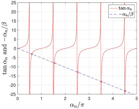
Figure 4. Characteristic values, ${\alpha }_n$, for $\beta =6.095\times {10}^{-2}$.

The experimental evidence shown in Figure 2a and Figure 3a supports the use of the solid–liquid interface equilibrium assumption, $C_{eq}=\gamma C_l$, because at the end of the first 24 h the concentration in the liquid seems to reach a constant value (see Figure 2a); it was only after the PBS medium was exchanged for a fresh one that the drug release continued (see Figure 2a). Condition (9) or its equivalent for the recursive delivery (17) includes the solid–liquid interface equilibrium assumption, and these conditions indicate that the rate of drug delivery to the liquid is time-varyiant, as it depends on the total mass of the drug in the liquid at the same instant. This concentration is proportional to the total mass inside the solid matrix due to the total mass balance of the total solid–liquid system. As a result of these conditions, the delivered mass with respect to the initial mass within the solid matrix tends to ${\left(1+\beta \right)}^{-1}$ as time tends to infinity (see Equation (32)), which is consistent with the experimental data, i.e., $m_l/m_{ini}\approx 0.621$ for $\beta =6.095\times {10}^{-2}$. Thus, for the particular experimental study case, when the drug concentration in the liquid is low, diffusion controls the delivery rate; however, as this concentration increases, the equilibrium plays a greater role, becoming the controlling mechanism as time increases.

The proposed models for single or recursive delivery are able to describe the delivered mass profile (see Figure 2a and Figure 3a), that is, the usual experimental measurement, and allows prediction of the concentration profile within the solid matrix, as shown in Figure 2b and Figure 3b. Notice that for the particular experimental study case, after each 24 h the profile concentration in the solid matrix is approximately constant, because the solid–liquid interface equilibrium has been reached. In addition, in order to validate the analytical solutions provided in Equation (32) for single release experiments and Equation (40) for recursive release experiments, numerical solutions of the proposed models were determined using an orthogonal collocation method; Figure 2a and Figure 3a show that the numerical and analytical solutions overlap.

6. Conclusions

In this work, a mathematical model to describe drug delivery from polymer coatings on implants was proposed. The model considers a unidirectional recursive diffusion process which follows Fick’s second law and considers the convective phenomena from the polymer matrix to the liquid where the drug is delivered as well as the polymer–liquid drug distribution equilibrium. The resulting model is solved using Laplace transformation for two scenarios: (1) a constant initial condition for a single drug delivery experiment; and (2) a recursive delivery process where the liquid medium is replaced with fresh liquid after a fixed period of time, causing a stepped delivery rate. Finally, the study case shows that these models can satisfactorily reproduce the experimental data, clarifying the predominant step in the control of drug release.

The proposed models for single and recursive release experiments presented in Section 2.1 and Section 2.2 have linear partial differential equations and boundary conditions; therefore, it was possible to obtain the analytical solutions provided in Equations (25), (31) and (32) for single release experiments, and Equations (39) and (40) for recursive release experiments. However, numerical methods are another option to solve these problems, and they become mandatory when extra phenomena need to be included in the drug release models in order to obtain satisfactory predictions, for instance, when swelling and degradation of the solid matrix become relevant, causing moving boundaries, or when a drug has more complex interactions such as biodegradation or adsorption, which produce non-linear terms in the model due to the reaction kinetics or adsorption isotherms.

References

- Quarterman, J.C.; Geary, S.M.; Salem, A.K. Evolution of drug-eluting biomedical implants for sustained drug delivery. Eur. J. Pharm. Biopharm. 2021, 159, 21–35. [Google Scholar] [CrossRef] [PubMed]
- Siepmann, J.; Siepmann, F. Mathematical modeling of drug delivery. Int. J. Pharm. 2008, 364, 328–343. [Google Scholar] [CrossRef] [PubMed]
- Higuchi, T. Mechanism of sustained-action medication. Theoretical analysis of rate of release of solid drugs dispersed in solid matrices. J. Pharm. Sci. 1963, 52, 1145–1149. [Google Scholar] [CrossRef]
- Ritger, P.L.; Peppas, N.A. A simple equation for description of solute release I. Fickian and non-fickian release from non-swellable devices in the form of slabs, spheres, cylinders or discs. J. Control. Release 1987, 5, 23–36. [Google Scholar] [CrossRef]
- Fu, Y.; Kao, W.J. Drug release kinetics and transport mechanisms of non-degradable and degradable polymeric delivery systems. Expert Opin. Drug Deliv. 2010, 7, 429–444. [Google Scholar] [CrossRef]
- Churchill, R.V. Operational Mathematics, 3rd ed.; McGraw-Hill: New York, NY, USA, 1972. [Google Scholar]
- Brown, J.W.; Churchill, R.V. Fourier Series and Boundary Value Problems, 8th ed.; McGrawHill: New York, NY, USA, 2012. [Google Scholar]
- Hernandez-Montelongo, J.; Naveas, N.; Degoutin, S.; Tabary, N.; Chai, F.; Spampinato, V.; Ceccone, G.; Rossi, F.; Torres-Costa, V.; Manso-Silvan, M.; et al. Porous silicon-cyclodextrin based polymer composites for drug delivery applications. Carbohydr. Polym. 2014, 110, 238–252. [Google Scholar] [CrossRef]
- França, C.G.; Plaza, T.; Naveas, N.; Santana, M.H.A.; Manso-Silván, M.; Recio, G.; Hernandez-Montelongo, J. Nanoporous silicon microparticles embedded into oxidized hyaluronic acid/adipic acid dihydrazide hydrogel for enhanced controlled drug delivery. Microporous Mesoporous Mater. 2021, 310, 110634. [Google Scholar] [CrossRef]
- Lagarias, J.C.; Reeds, J.A.; Wright, M.H.; Wright, P.E. Convergence Properties of the Nelder–Mead Simplex Method in Low Dimensions. SIAM J. Optim. 1998, 9, 112–147. [Google Scholar] [CrossRef] [Green Version]
Publisher’s Note: MDPI stays neutral with regard to jurisdictional claims in published maps and institutional affiliations. |
© 2022 by the authors. Licensee MDPI, Basel, Switzerland. This article is an open access article distributed under the terms and conditions of the Creative Commons Attribution (CC BY) license (https://creativecommons.org/licenses/by/4.0/).