Quantile-Zone Based Approach to Normality Testing

Abstract

Normality testing remains an important issue for researchers, despite many solutions that have been published and in use for a long time. There is a need for testing normality in many areas of research and application, among them in Quality control, or more precisely, in the investigation of Shewhart-type control charts. We modified some of our previous results concerning control charts by using the empirical distribution function, proper choice of quantiles and a zone function that quantifies the discrepancy from a normal distribution. That was our approach in constructing a new normality test that we present in this paper. Our results show that our test is more powerful than any other known normality test, even in the case of alternatives with small departures from normality and for small sample sizes. Additionally, many test statistics are sensitive to outliers when testing normality, but that is not the case with our test statistic. We provide a detailed distribution of the test statistic for the presented test and comparable power analysis with highly illustrative graphics. The discussion covers both the cases for known and for estimated parameters.

1. Introduction

It is well known that even though many methods for preliminarily checking the normality of distribution, such as box plot, quantile–quantile (Q–Q) plot, histogram or observing the values of empirical skewness and kurtosis, are available. However, the results of those methods are inconclusive or not precise enough [1,2,3]. Considering the importance of the level of certainty with which we can claim the normal distribution of the sample’s characteristic X, the most formal and precise methods are needed. Normality tests are shown to yield the best results, based on which one can, with a certain level of significance, determine not only if the sample elements fit the normal distribution at all but can also determine the measure of concordance with normal distribution [1,4,5,6,7,8,9]. Because of those properties, a wide range of normality tests was developed [1,3,4,5,6,7,8,9,10,11,12,13,14,15,16,17].

The next challenge was determining which test satisfies as many of the criteria for statistical tests as possible. For instance, a test primarily has to be powerful. Usually, the power of the test is calculated only through simulations [2,5,6,9,10,11,12,13,14,15,16]. Often, so is the distribution of the test statistic [2,5,9]. That is due to conditions for the weak law of large numbers or the central limit theorem not being satisfied. Hence, the problem of determining the distribution of the test statistic remains unsolved [2,9,18,19,20]. The next challenge is knowing the correct amount of simulations [20,21,22]. Additionally, the power of the test variates for different groups of alternative distributions (symmetric, asymmetric) and different sample sizes [9,10,11,12,13,14,15,16].

On certain occasions, some of the normality tests are more powerful than the other tests, yet, their application seems to be much slower and hard to implement. That diminishes their contribution importance [1,3,6,10,11,17]. Another issue is that many tests seem to have the power that differs for symmetric and asymmetric alternative distributions. We also need to consider some generally less powerful tests because some (such as the Jarque–Bera test or D’Agostino test) are useful [10,11]. For instance, overcoming mentioned problems can cause overcoming many other issues.

Currently, the most used normality tests are the Kolmogorov–Smirnov test and the Chi-squared test, followed by the Shapiro–Wilk test and the Anderson–Darling test [1,2,10,11,12,13,14,15,16], even though some other tests are more powerful [10]. That indicates how important the simplicity of implementation and fast performance are, even for low power tests [5,10].

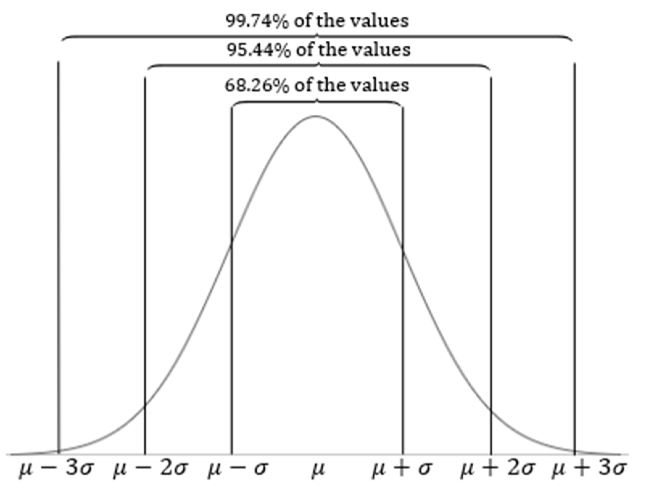
In this paper, our goal is to contribute to this topic by developing a new normality test based on the 3σ rule. We define a new zone function that quantifies the deviation of the empirical distribution function (EDF) from the cumulative distribution function (CDF) for the obtained sample’s characteristic. The test statistic is the mean of the values of the zone function with sample elements as arguments.

In [23,24], we developed new Shewhart-type control charts [25,26] based on the 3σ rule. The basic idea is to use the empirical distribution function for the means of all the samples to be controlled. We form control lines by using quantiles of those means for normal $N\left(\mu ,\frac{{\sigma }^2}{n}\right)$ distribution. That is due to a normal distribution $N\left(\mu ,{\sigma }^2\right)$ being assumed and used in quality control and central limit theorem [24,26].

Using the same principle in individual analyzing samples, the same control chart is used for a preliminary analysis of the normality of the referent sample distribution. Here the variance of the distribution is σ² Defining the proper statistic through adequate function for quantifying the level of sample deviation from the normal distribution based on the control chart zones enables us to do the above-mentioned [23].

These were our first steps in the subject that brought us to the idea of developing a new test of normality. That consists of modifying some ideas in [23,24].

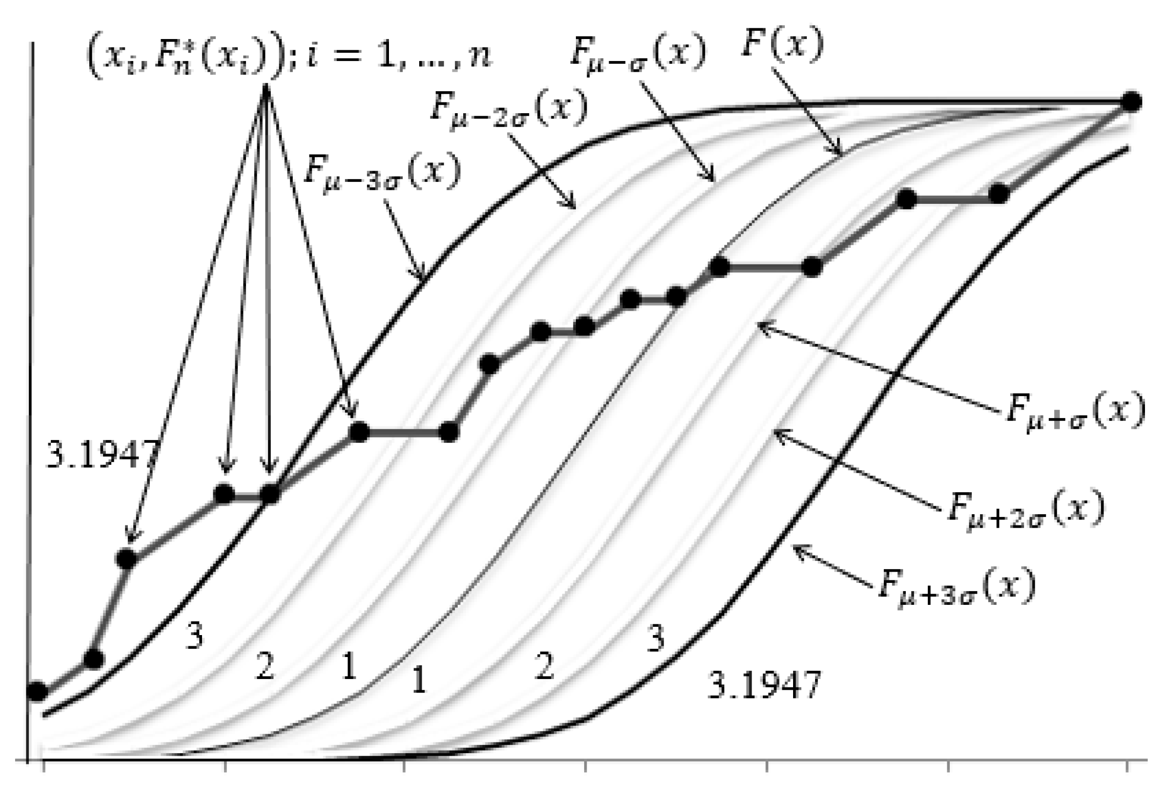
In this paper, we define the zone function given in [23] with a modification that will be applicable in the case where the sample is not “in a control” state since in normality testing, unlike in quality control, some outliers do not essentially mean rejection of the null hypothesis. The outliers do not affect significant change in our test statistic value unless there are many of them. In many other tests, the opposite happens, which causes the rejection of the null hypothesis even when it should not be.

Finally, we provide some main characteristics of the test statistic’s distribution and table for various probabilities and sample sizes and the power analysis with a simulation study. We discuss both cases for known or estimated parameters. We use the sample mean and corrected sample variance, and both are unbiased, reliable, etc. [2,5]. Conclusions that make the test statistic better than others rely on our results obtained through Monte Carlo simulations and the results and comparative analysis available for other tests in [5,6,9,10,11,12,13,14,15,16].

An important notion is that multivariate normality testing is a topic that is still in need of research because of the problems of identifying the proper test in certain circumstances [1,27,28]. Even though many results were obtained [1,27], new approaches are being developed and improved [27,28,29,30]. The test we developed in this paper can be a solid background for continuing the research in multivariate normality testing by extending our solution or investigating some new ones based on similar principles.

2. Quantile-Zone Based Approach to Normality Testing for Known Parameters

2.1. The Test Statistic and Basic Properties

Let $X_1, X_2, \dots , X_n; n\in \mathbb{N}$ be the simple random sample of characteristic $X:N\left(\mu , {\sigma }^2\right)$,

$$F\left(x\right)={\int }_{-\infty }^x\frac{1}{\sqrt{2\pi }\sigma }{e}^{-\frac{{\left(x-\mu \right)}^2}{2{\sigma }^2}}dx; x\in ℝ$$

its CDF, $F_{\mu \pm i\sigma }\left(x\right); x\in ℝ; i=1, 2, 3$ are CDFs for normal distribution $N\left(\mu \pm i\sigma \right)$ and

$$F_n^{*}\left(x\right)=\frac{1}{n}{\displaystyle \sum }_{i=1}^{n}I\left(X_i\le x\right);x\in ℝ$$

sample’s EDF (I is the event indicator; it is equal to 1 if the argument event is the realized one and 0 otherwise). Normal distribution variates are distributed by the 3σ rule, hence the sample elements will be approximately distributed by it. The 3σ rule is interpretable as per Figure 1.

Figure 1. The $3\sigma$ rule.

Hence, since $F_n^{*}\left(x\right)\to F\left(x\right)\left(n\to +\infty \right)$ [18], we have that:

• $F_{\mu +\sigma }\left(X_i\right)\le F_n^{*}\left(X_i\right)<F\left(X_i\right)$, i.e., $F\left(X_i\right)<F_n^{*}\left(X_i\right)\le F_{\mu -\sigma }\left(X_i\right)$, is true for 34.13% of sample elements
• $F_{\mu +2\sigma }\left(X_i\right)\le F_n^{*}\left(X_i\right)<F_{\mu +\sigma }\left(X_i\right)$, i.e., $F_{\mu -\sigma }\left(X_i\right)<F_n^{*}\left(X_i\right)\le F_{\mu -2\sigma }\left(X_i\right)$, is true for 13.59% of sample elements
• $F_{\mu +3\sigma }\left(X_i\right)\le F_n^{*}\left(X_i\right)<F_{\mu +2\sigma }\left(X_i\right)$, i.e., $F_{\mu -2\sigma }\left(X_i\right)<F_n^{*}\left(X_i\right)\le F_{\mu -3\sigma }\left(X_i\right)$, is true for 2.15% of sample elements
• $F_n^{*}\left(X_i\right)<F_{\mu +3\sigma }\left(X_i\right)$, i.e., $F_n^{*}\left(X_i\right)>F_{\mu -3\sigma }\left(X_i\right)$, is true for 0.13% of sample elements

where $i=\overline{1,n}$.

We define a function

$$zone\left(x\right)=\left\{\begin{array}{cc}1;& F_{\mu +\sigma }\left(x\right)\le F_n^{*}\left(x\right)<F\left(x\right)\vee F\left(x\right)<F_n^{*}\left(x\right)\le F_{\mu -\sigma }\left(x\right)\\ 2;& F_{\mu +2\sigma }\left(x\right)\le F_n^{*}\left(x\right)<F_{\mu +\sigma }\left(x\right)\vee F_{\mu -\sigma }\left(x\right)<F_n^{*}\left(x\right)\le F_{\mu -2\sigma }\left(x\right)\\ 3;& F_{\mu +3\sigma }\left(x\right)\le F_n^{*}\left(x\right)<F_{\mu +2\sigma }\left(x\right)\vee F_{\mu -2\sigma }\left(x\right)<F_n^{*}\left(x\right)\le F_{\mu -3\sigma }\left(x\right)\\ 3.1947;& F_n^{*}\left(x\right)<F_{\mu +3\sigma }\left(x\right)\vee F_n^{*}\left(x\right)>F_{\mu -3\sigma }\left(x\right)\end{array};x\in ℝ\right..$$

(1)

The definition of the zone function is shown in Figure 2.

Figure 2. The zone function (1) illustrated.

Let $Y_1,Y_2,\dots ,Y_n$ be ordered sample $X_1, X_2, \dots , X_n$ in the order from the smallest to the largest value, and

$$n_{\max }={\displaystyle \sum }_{i=1}^{n}I\left(X_i=\underset{j=\overline{1,n}}{\max }{X}_j\right).$$

The distribution of statistic $zone\left(Y_i\right);i=\overline{1,n_{\max }-1}$ is given with the

$$zone\left(Y_i\right):\left(\begin{array}{cccc}1& 2& 3& 3.1947\\ 0.6826& 0.2718& 0.0430& 0.0026\end{array}\right),$$

and we have $E\left(zone\left(Y_i\right)\right)=1.3635$ and $Var\left(zone\left(Y_i\right)\right)=0.3242$, while the standard deviation is ${\sigma }_{zone\left(Y_i\right)}=0.5694$. For $Y_k,k=\overline{n_{\max },n}$ we have $P\left(zone\left(Y_k\right)=3.1947\right)=1$. The choice of the value $3.1947$ is explained by the expressions

$$F^{-1}\left(\frac{F\left(3\right)+\underset{x\to +\infty }{\lim }F\left(x\right)}{2}\right)=3.1947$$

and

$$F^{-1}\left(\frac{\underset{x\to +\infty }{\lim }F\left(x\right)+F\left(-3\right)}{2}\right)=-3.1947.$$

Though any other value can be taken as well, this way we ensure the analogy with the $3\sigma$ rule that we started with.

Now we define the statistic

$${\overline{V}}_n=\frac{1}{n}{\displaystyle \sum }_{i=1}^{n}zone\left(X_i\right).$$

(2)

To calculate the expectation $E$ and variance (dispersion) $Var$ of ${\overline{V}}_n$ correctly we need to consider that $F_n^{*}\left(Y_n\right)=F_n^{*}\left(\underset{j=\overline{1,n}}{\max }{X}_j\right)=1$, which leads to $zone\left(Y_n\right)=zone\left(\underset{j=\overline{1,n}}{\max }{X}_j\right)=3.1947$. Then we achieve:

$$E\left({\overline{V}}_n\right)=E\left(\frac{1}{n}{\displaystyle \sum }_{i=1}^{n}zone\left(X_i\right)\right)=\frac{1}{n}\left({\displaystyle \sum }_{i=1}^{n}E\left(zone\left(X_i\right)|X_i\ne \underset{j=\overline{1,n}}{\max }{X}_j\right)+n_{\max }E\left(\underset{j=\overline{1,n}}{\max }{X}_j\right)\right)$$

$$=\frac{\left(n-n_{\max }\right)·1.3635+n_{\max }·3.1947}{n},$$

as well as:

$$Var\left({\overline{V}}_n\right)=E\left({\overline{V}}_n^2\right)-{\left(E\left({\overline{V}}_n\right)\right)}^2=E\left({\left(\frac{1}{n}{\displaystyle \sum }_{i=1}^{n}zone\left(X_i\right)\right)}^2\right)-{\left(\frac{\left(n-n_{\max }\right)·1.3635+n_{\max }·3.1947}{n}\right)}^2$$

$$=E\left({\left(\frac{1}{n}{\displaystyle \sum }_{i=1}^{n}zone\left(Y_i\right)\right)}^2\right)-{\left(\frac{\left(n-n_{\max }\right)·1.3635+n_{\max }·3.1947}{n}\right)}^2$$

$$\begin{gathered} =\frac{1}{n^2}({\displaystyle \sum }_{i=1}^{n-n_{\max }}E\left(zone{\left(Y_i\right)}^2\right)+{\displaystyle \sum }_{i=n-n_{\max }+1}^{n}E\left(zone{\left(Y_i\right)}^2\right) \\ +2\left({\displaystyle \sum }_{i=1}^{n-n_{\max }}{\displaystyle \sum }_{\begin{array}{c}k=1\\ k\ne i\end{array}}^{n-n_{\max }}E\left(zone\left(Y_i\right)·zone\left(Y_k\right)\right)+2{\displaystyle \sum }_{i=1}^{n-n_{\max }}{\displaystyle \sum }_{k=n-n_{\max }+1}^{n}E\left(zone\left(Y_i\right)·zone\left(Y_k\right)\right) \\ +{\displaystyle \sum }_{i=n-n_{\max }+1}^n{\displaystyle \sum }_{\begin{array}{c}k=n-n_{\max }+1\\ k\ne i\end{array}}^{n}E\left(zone\left(Y_i\right)·zone\left(Y_k\right)\right)\right))-{\left(\frac{\left(n-n_{\max }\right)1.3635+n_{\max }3.1947}{n}\right)}^2 \end{gathered}$$

$$\begin{gathered} =\frac{1}{n^2}\left(\left(n-n_{\max }\right)2.1833+n_{\max }{3.1947}^2+2\left(\left(\begin{array}{c}n-n_{\max }\\ 2\end{array}\right){1.3635}^2+2n_{\max }\left(n-n_{\max }\right)1.3635·3.1947\right) \\ +\left(\begin{array}{c}{n}_{\max }\\ 2\end{array}\right){3.1947}^2\right)-{\left(\frac{\left(n-n_{\max }\right)1.3635+n_{\max }3.1947}{n}\right)}^2 \end{gathered}$$

$$\begin{gathered} =\frac{1}{n^2}\left(\left(n-n_{\max }\right)2.1833+n_{\max }{3.1947}^2+\left(n-n_{\max }\right)\left(n-n_{\max }-1\right){1.3635}^2+4n_{\max }\left(n-n_{\max }\right)1.3635·3.1947 \\ +n_{\max }\left(n_{\max }-1\right){3.1947}^2-{\left(n-n_{\max }\right)}^2{1.3635}^2-2n_{\max }\left(n-n_{\max }\right)1.3635·3.1947 \\ -n_{\max }^2·{3.1947}^2\right) \end{gathered}$$

$$\begin{gathered} =\frac{1}{n^2}\left(\left(n-n_{\max }\right)2.1833+n_{\max }{3.1947}^2-\left(n-n_{\max }\right){1.3635}^2+2n_{\max }\left(n-n_{\max }\right)1.3635·3.1947-n_{\max }{3.1947}^2\right) \\ =\frac{\left(n-n_{\max }\right)\left(0.3243+n_{\max }8.7119\right)}{n^2}. \end{gathered}$$

Since the normal distribution of the sample is assumed, the frequency of the maximal value is most often $1$. In that case, we have

$$E\left({\overline{V}}_n\right)=\frac{\left(n-1\right)1.3635+3.1947}{n}$$

and

$$Var\left({\overline{V}}_n\right)=\frac{\left(n-1\right)\left(0.3242+8.7119\right)}{n^2}=\frac{\left(n-1\right)9.0361}{n^2}.$$

2.2. Distribution of the Test Statistic and the Testing Procedure

The expectation and variance of the statistic ${\overline{V}}_n;n\in \mathbb{N}$ are finite, hence, based on the weak law of large numbers statistic, ${\overline{V}}_n$ converges to its expectation [2,19], i.e.,

$${\overline{V}}_n=\frac{1}{n}{\displaystyle \sum }_{i=1}^{n}zone\left(X_i\right)\to \frac{1}{n}{\displaystyle \sum }_{i=1}^{n}E\left(zone\left(X_i\right)\right)=\frac{\left(n-n_{\max }\right)·1.3635+n_{\max }·3.1947}{n}\to 1.3635 \left(n\to +\infty \right).$$

The empirical distribution function, i.e., its value for sample elements as arguments, depends on the sample size and frequency of each sample element less than or equal to the referent one. This means that the sample $F_n^{*}\left(X_1\right),F_n^{*}\left(X_2\right),\dots ,F_n^{*}\left(X_n\right);n\in \mathbb{N}$ has mutually dependent random variables as elements. Hence, the same goes for the sample $zone\left(X_1\right),zone\left(X_2\right),\dots ,zone\left(X_n\right);n\in \mathbb{N}$. In that case, the central limit theorem does not apply to our statistic ${\overline{V}}_n$ [2] and its distribution is determinable only via simulations.

In the following table, we offer the distribution table of statistic ${\overline{V}}_n$, i.e., the values $q$ obtained from

$$P({\overline{V}}_n\le q|X:N\left(\mu ,{\sigma }^2\right))=p.$$

Here, $n$ is the size of the sample. It is impossible to simulate the critical values for every sample size. For the sample sizes, or values $p$ and $q$, that are not available in the table, a convenient approximation should be used, for example, the bisection method. We used 100,000 Monte Carlo simulations for each sample size in Table 1.

Table 1. $F_{{\overline{V}}_n}\left(q\right)=P\left({\overline{V}}_n\le q\right)=p$—Known parameters.

$\mathit{n}$	$\mathit{p}$
	0.01	0.025	0.05	0.1	0.15	0.2	0.5	0.8	0.85	0.9	0.95	0.975	0.99
10	1.0028	1.0070	1.0140	1.0280	1.0421	1.0561	1.1402	1.2315	1.2657	1.2999	1.3709	1.4480	1.5656
20	1.0013	1.0031	1.0062	1.0125	1.0187	1.0249	1.0624	1.0998	1.1061	1.1208	1.1473	1.1636	1.2048
30	1.0008	1.0020	1.0040	1.0080	1.0120	1.0160	1.0402	1.0643	1.0683	1.0723	1.0910	1.1023	1.1223
50	1.0005	1.0012	1.0024	1.0047	1.0071	1.0094	1.0235	1.0376	1.0399	1.0423	1.0495	1.0583	1.0635
100	1.0002	1.0006	1.0012	1.0023	1.0035	1.0046	1.0115	1.0185	1.0196	1.0208	1.0219	1.0275	1.0308
200	1.0001	1.0003	1.0006	1.0012	1.0017	1.0023	1.0057	1.0091	1.0096	1.0102	1.0108	1.0126	1.0148
300	1.0001	1.0002	1.0004	1.0008	1.0011	1.0015	1.0038	1.0060	1.0064	1.0068	1.0072	1.0082	1.0098
500	1.0000	1.0001	1.0002	1.0004	1.0007	1.0009	1.0022	1.0036	1.0039	1.0041	1.0043	1.0047	1.0058
1000	1.0000	1.0000	1.0001	1.0002	1.0003	1.0004	1.0011	1.0018	1.0019	1.0020	1.0022	1.0022	1.0028
1500	1.0000	1.0000	1.0000	1.0001	1.0002	1.0003	1.0008	1.0012	1.0012	1.0013	1.0014	1.0014	1.0018
2000	1.0000	1.0000	1.0000	1.0001	1.0002	1.0002	1.0006	1.0009	1.0009	1.0010	1.0011	1.0011	1.0013

The critical region for testing the null hypothesis $H_0\left(X:N\left(\mu ,{\sigma }^2\right)\right)$ is given with the interval $W=\left[1,c_1\right]\bigcup \left[c_2,3,1947\right]$, where $c_1$ and $c_2$ are determined from the condition

$$P\left({\overline{V}}_n\le c_1|H_0\right)=P({\overline{V}}_n\ge c_2|H_0)=\frac{\alpha }{2},$$

where $\alpha$ is the level of significance. That is due to the test statistic relying on the $3\sigma$ rule properties. Namely, we have a two-tailed critical region because of the “perfect fit” case. In that case, certain uniform alternative distributions yield the sample such that its EDF will be entirely inside the band $\left[F_{\mu +\sigma }\left(x\right),F_{\mu -\sigma }\left(x\right)\right];x\in ℝ$. However, the distribution is not the normal one.

For instance, if we observe the sample

$$\mu +\left(-3.5+\frac{7k}{n}\right)\sigma ; n\in \mathbb{N}, k=\overline{0,n}$$

(3)

its EDF will be

$$F_n^{*}\left(x\right)=\left\{\begin{array}{cc}0;& x<\mu -3.5\sigma \\ \frac{j}{n};& \mu +\left(-3.5+\frac{7(j-1)}{n}\right)\sigma \le x<\mu +\left(-3.5+\frac{7j}{n}\right)\sigma ; j=\overline{1,n}\end{array}.\right.$$

In this case, for any positive integer $n$, EDF is inside the band $\left[F_{\mu +\sigma }\left(x\right),F_{\mu -\sigma }\left(x\right)\right];$ for any $x\in ℝ$. However, the sampling distribution is the uniform one, and as such, it should cause hypothesis rejection [30]. We can also say that any sampling distribution does not significantly differ from the distribution given with (3), as long as its EDF is inside the band $\left[F_{\mu +\sigma }\left(x\right),F_{\mu -\sigma }\left(x\right)\right];$ for any $x\in ℝ$.

If the empirical value ${\overline{v}}_n$ of test-statistic ${\overline{V}}_n$ is inside the critical region $W$, we reject the null hypothesis $H_0\left(X:N\left(\mu ,{\sigma }^2\right)\right)$.

The p-value for this test is calculated by

$$p=2\min \left\{P\left({\overline{V}}_n\le {\overline{v}}_n|H_0\right),P\left({\overline{V}}_n\ge {\overline{v}}_n|H_0\right)\right\}$$

and then compared to the level of significance $\alpha$. If $p\le \alpha$ the null hypothesis is rejected.

Ad hoc, this way of testing the normality hypothesis indicates many of its advantages. The method of its construction gives tools for checking the frequency of sample elements inside some interval we observe. It checks out if the range of the sample is concordant with the one in the theoretical model. On some level, it is even sensitive to outliers because more of them will increase the likelihood of the hypothesis rejection, and a few of them (especially for large-sized samples) will not affect the decision-making. That is important since, in theory, normal variates absolute values can be as high as any positive number [31].

To be more precise, we note that our test statistic is invariant to minor changes such as increasing or decreasing some sample element’s value in a manner that its order statistic remains the same. On the other hand, the test statistic identifies essential changes (the best indicated by the order statistics realized values changes) as a significant or insignificant violator of the normality of distribution. The test statistic is also sensitive to the sample elements’ dependence anomalies since it does not examine only the position of each sample element but also its correspondence to other sample elements. The fact that the EDF values are determined through the order statistics of the sample elements, as well as their frequency in the observed sample [1], substantiates these conclusions. Additionally, the zone function ensures proper discrepancy measurement, i.e., the test statistic registers the density of the sample elements inside the intervals defined by the zone function ($3\sigma$ rule).

2.3. Power Analysis

In this section, we offer power analysis results obtained through Monte Carlo simulations of the distribution of statistic ${\overline{V}}_n$ with 10,000 runs (samples) for various sample sizes and alternative distributions. The null distribution is $N\left(0,1\right)$. Simulations are performed using MATLAB with the random number generation algorithms and modeling methods implemented in it. Many of the distributions can be modeled in MATLAB with the special command (“normrnd”, “chi2rnd”, “betarnd” etc.), however, not all the distributions are available [32]. In that case, we used the inverse function method [21,22,31].

As usual, symmetric and asymmetric alternative distributions are observed separately and empirical powers are calculated for different sample sizes. The choice of parameters is such that these distributions overlap with the normal distribution as much as possible [31], even though in other papers, for a lot of chosen alternative distributions (or their parameters), some of the preliminary analysis methods would serve the purpose [10,11,13,14].

Calculating the power values for a chosen alternative distribution is performed in the following way:

• Modeling the sample $x_1,x_2,\dots ,x_n$ of chosen alternative distribution for the observed sample size $n$;
• Determining the EDF $F_n^{*}\left(x\right)$ for obtained sample, and then calculating the values $zone\left(x_1\right),zone\left(x_2\right),\dots ,zone\left(x_n\right)$ and finally, we calculate:
  • ${\overline{v}}_n=\frac{1}{n}{\displaystyle \sum }_{i=1}^{n}zone\left(x_i\right);$
• Repeating previous steps 10,000 times gives us the sample ${\overline{v}}_{n;1}, {\overline{v}}_{n;2},\dots ,{\overline{v}}_{n;\mathrm{10,000}}$;
• Determining the new sample EDF ${\overline{F}}_{\mathrm{10,000}}^{*}\left(x\right)$;
• $\mathrm{Power}={\overline{F}}_{\mathrm{10,000}}^{*}\left(c_1\right)+\left(1-{\overline{F}}_{\mathrm{10,000}}^{*}\left(c_2\right)\right)$ where $c_1$ and $c_2$ are critical values for the level of significance $\alpha =0.05$.

Note that the number of simulations is not higher since we simulated the distribution of the test statistics (for null distribution of $X$) for both 10,000 and 100,000 simulations, and the results are asymptotically identical. Though the same does not necessarily hold for other distributions, 10,000 Monte Carlo simulations are proven to be satisfactory [20] (pp. 97–116).

Note that the Quantile-Zone test has a smaller power value for the normal alternative distributions, though its power is still high enough in most cases. Additionally, lower variance in normal alternative distributions causes its power value to be lower. That does not mean our test should not be used in the mentioned cases since its power value is still better than any other known normality test [5,6,9,10,11,12,13,14,15,16].

Positive kurtosis does not affect the power value of the test, as can be seen in Figure 3 and Table 2. Namely, the Laplace $\left(0, 1\right)$ distribution has a higher kurtosis than $N\left(0, 1\right)$, but its power value is high.

Figure 3. PDFs of symmetric alternative distributions compared to the PDF of null $N\left(0,1\right)$ distribution.

Table 2. Empirical powers of statistic ${\overline{V}}_n$ for symmetric alternative distributions for the level of significance $\alpha =0.05$.

Distribution	$\mathit{n}$
	10	20	30	50	100	200
$\mathit{N}\left(\mathbf{0}, {\mathbf{0.5}}^{\mathbf{2}}\right)$	0.0001	0.0826	0.3059	0.6623	0.9553	0.9994
$\mathit{N}\left(\mathbf{0}, {\mathbf{1.5}}^{\mathbf{2}}\right)$	0.3017	0.5388	0.7154	0.8363	0.9140	0.9702
${\mathit{t}}_{\mathbf{2}}$	0.3206	0.6786	0.8479	0.9544	0.9975	1
Logistic (0, 1)	0.4657	0.7966	0.9193	0.9838	0.9990	1
Cauchy (0, 1)	0.5801	0.9328	0.9875	0.9995	1	1
Tukey (0.14)	0.7503	0.9693	0.9934	0.9995	1	1
Laplace (0, 1)	0.5181	0.8364	1	1	1	1
$\mathit{U}\left(-\mathbf{3.5}, \mathbf{3.5}\right)$	1	1	1	1	1	1
Average	0.4921	0.7294	0.8462	0.9295	0.9832	0.9962

For asymmetric alternative distributions, our test has the lowest power value (compared to other asymmetric alternative distributions) for Gumbel $\left(0, 1\right)$ distribution and $N\left(1, 1\right)$ distribution (Figure 4). For small sample sizes, the test performs better in the case of normal distribution than in the case of Gumbel distribution, but for $n>200$, it is the opposite. It is important to note that for $n>200$, the power of the Quantile-Zone test is asymptotically close to 1 in both cases (Table 3).

Figure 4. PDFs of asymmetric alternative distributions compared to the PDF of null $N\left(0,1\right)$ distribution.

Table 3. Empirical powers of statistic ${\overline{V}}_n$ for asymmetric alternative distributions for the level of significance $\alpha =0.05$.

Distribution	$\mathit{n}$
	10	20	30	50	100	200
Gumbel (0, 1)	0.1257	0.3573	0.5581	0.7349	0.9236	0.9939
$\mathit{N}\left(\mathbf{1},\mathbf{1}\right)$	0.4930	0.8026	0.8724	0.9255	0.9668	0.9851
Lognormal (0, 1)	0.7928	0.9993	1	1	1	1
Pareto (0.0001, 1)	0	1	1	1	1	1
${\mathit{\chi }}_{\mathbf{1}}^{\mathbf{2}}$	0.9209	1	1	1	1	1
Gamma (2, 1)	0.9946	1	1	1	1	1
Beta (2, 1.5)	0.1900	1	1	1	1	1
Weibull (1, 2)	0.5884	1	1	1	1	1
Burr (3, 1)	1	1	1	1	1	1
Average	0.5673	0.9066	0.9367	0.9623	0.9878	0.9977

The results (Table 2 and Table 3) show that statistic ${\overline{V}}_n$ performs very well. Namely, based on the results obtained in [5,6,9,10,11,12,13,14,15,16], it has higher power values than the usually used normality tests or any other discussed test for most of the known alternative distribution. The conclusion holds even for small sample sizes. Though the comparison is difficult to perform due to the variety of observed alternative distributions, sample sizes and the used number of simulations (in some cases, the level of significance is not 0.05 [11]), it is still easy to see the advantage of our test.

3. Quantile-Zone-Based Approach to Normality Testing for Estimated Parameters

3.1. Distribution and Properties of the Test-Statistic

Theoretically, when we estimate parameters $\mu$ and ${\sigma }^2$ with

$${\overline{X}}_n=\frac{1}{n}{\displaystyle \sum }_{i=1}^n{X}_i$$

and

$${\tilde{S}}_n^2=\frac{1}{n-1}{\displaystyle \sum }_{i=1}^n{\left(X_i-{\overline{X}}_n\right)}^2,$$

respectively, the distribution of statistic ${\overline{V}}_n$, as well as its basic properties, remains the same. However, empirically, that never happens. Namely, even though the sample is the sample of the characteristic $X:N\left(\mu ,{\sigma }^2\right)$, we shall (almost) always have ${\overline{X}}_n=\mu \pm {\epsilon }_1$ and ${\tilde{S}}_n^2={\sigma }^2\pm {\epsilon }_2$. Errors ${\epsilon }_1$ and ${\epsilon }_2$ are then cumulated while calculating the values $zone\left(X_i\right);i=1,\dots ,n$, i.e., the empirical value of ${\overline{V}}_n$. Hence, the distribution of ${\overline{V}}_n$ is slightly changed. Monte Carlo simulations give us the results in Table 4.

Table 4. $F_{{\overline{V}}_n}\left(q\right)=P\left({\overline{V}}_n\le q\right)=p$—Estimated parameters.

$\mathit{n}$	$\mathit{p}$
	0.01	0.025	0.05	0.1	0.15	0.2	0.5	0.8	0.85	0.9	0.95	0.975	0.99
10	1.0023	1.0057	1.0113	1.0226	1.0339	1.0452	1.1130	1.1807	1.1920	1.2033	1.2146	1.2316	1.2844
20	1.0012	1.0029	1.0057	1.0114	1.0171	1.0227	1.0568	1.0910	1.0966	1.1023	1.1080	1.1236	1.1453
30	1.0008	1.0019	1.0038	1.0076	1.0114	1.0152	1.0379	1.0607	1.0645	1.0683	1.0720	1.0823	1.0974
50	1.0005	1.0012	1.0023	1.0046	1.0068	1.0091	1.0228	1.0364	1.0387	1.0409	1.0433	1.0500	1.0586
100	1.0002	1.0006	1.0012	1.0023	1.0034	1.0045	1.0114	1.0181	1.0193	1.0204	1.0216	1.0246	1.0293
200	1.0001	1.0003	1.0006	1.0012	1.0017	1.0023	1.0056	1.0090	1.0096	1.0102	1.0108	1.0117	1.0145
300	1.0001	1.0002	1.0004	1.0008	1.0011	1.0015	1.0037	1.0060	1.0064	1.0068	1.0071	1.0076	1.0095
500	1.0000	1.0001	1.0002	1.0004	1.0007	1.0009	1.0022	1.0036	1.0039	1.0041	1.0043	1.0044	1.0058
1000	1.0000	1.0000	1.0001	1.0002	1.0003	1.0004	1.0011	1.0018	1.0019	1.0020	1.0022	1.0022	1.0028
1500	1.0000	1.0000	1.0000	1.0001	1.0002	1.0003	1.0008	1.0012	1.0012	1.0013	1.0014	1.0014	1.0018
2000	1.0000	1.0000	1.0000	1.0001	1.0002	1.0002	1.0006	1.0009	1.0009	1.0010	1.0011	1.0011	1.0013

We can see that the values are smaller when the zone function is defined with estimated parameters because, for empirically obtained samples, most often the sample mean ${\overline{X}}_n$ and variance ${\tilde{S}}_n^2$ are better indicators of the expected value and the dispersion of obtained sample elements than values $\mu$ and ${\sigma }^2$ that are used for sample modeling. The difference in the distribution is smaller for larger sample sizes. For $n>500$ the distributions are identical. A graphical representation of both variants is given in Figure 5.

Figure 5. Statistic ${\overline{V}}_n$ values $q$ for various sample sizes $n$ and probabilities $p$: (a) Parameters $\mu$ and ${\sigma }^2$ are known; (b) Parameters $\mu$ and ${\sigma }^2$ are estimated with ${\overline{X}}_n$ and ${\tilde{S}}_n^2$, respectively.

3.2. Power Analysis

When parameters are estimated, smaller values of the statistic ${\overline{V}}_n$ indicate higher values of power function for any alternative distribution. That can be seen in the following tables and figures.

Usually, the small sample size ($n<30$) affects the power of the test to be lower. That is due to small samples not giving enough information about the characteristic $X$ [33]. That is also the case for our Quantile-Zone test statistic. However, its power is still high for most alternative distributions and even for $n=10$. The exceptions are normal $N\left(0, {0.5}^2\right)$ and Pareto (0.0001, 1) distributions. In Table 5, we can see that the Quantile-Zone test identifies the $N\left(0, {0.5}^2\right)$ distribution as $N\left(0, 1\right)$ for $n=10$. With the increase in the sample size, that is not the case. The same holds for the Pareto distribution, where we can say that the sample of the size $n=10$ is too small since, for $n=20$, the empirical power is 1.

Table 5. Empirical power of statistic ${\overline{V}}_n$ where parameters are estimated, for various sample sizes with the level of significance $\alpha =0.05$—Symmetric alternative distributions.

Distribution	n
	10	20	30	50	100	200
$\mathit{N}\left(\mathbf{0}, {\mathbf{0.5}}^{\mathbf{2}}\right)$	0.1898	0.3859	0.5728	0.7942	0.9731	0.9996
$\mathit{N}\left(\mathbf{0}, {\mathbf{1.5}}^{\mathbf{2}}\right)$	0.6464	0.7257	0.7756	0.8367	0.9141	0.9704
${\mathit{t}}_{\mathbf{2}}$	0.6607	0.7926	0.8831	0.9613	0.9980	1
Logistic (0, 1)	0.7884	0.8943	0.9406	0.9847	0.9989	1
Cauchy (0, 1)	0.8406	0.9627	0.9902	0.9996	1	1
Tukey (0.14)	0.9361	0.9863	0.9934	0.9959	1	1
Laplace (0, 1)	0.7851	0.9442	1	1	1	1
$\mathit{U}\left(-\mathbf{3.5}, \mathbf{3.5}\right)$	1	1	1	1	1	1
Average	0.7309	0.8365	0.8945	0.9466	0.9855	0.9962

When we estimate parameters, the problem is by far smaller. Namely, we can see a noticeable increase in the power for both mentioned alternative distributions (Table 5 and Table 6, Figure 6 and Figure 7). The difference in the values of test statistics in the case of estimated parameters as appose to one of the known values of parameters is smaller for larger sample sizes. The same holds for the power functions. The following tables illustrate this.

Table 6. Empirical power of statistic ${\overline{V}}_n$ where parameters are estimated for various sample sizes with the level of significance $\alpha =0.05$—Asymmetric alternative distributions.

Distribution	$\mathit{n}$
	10	20	30	50	100	200
Gumbel (0, 1)	0.3508	0.5029	0.6116	0.7601	0.9262	0.9942
$\mathit{N}\left(\mathbf{1}, \mathbf{1}\right)$	0.7593	0.8616	0.9112	0.9378	0.9669	0.9864
Lognormal (0, 1)	0.9833	1	1	1	1	1
Pareto (0.0001, 1)	0.9999	1	1	1	1	1
${\mathit{\chi }}_{\mathbf{1}}^{\mathbf{2}}$	0.9927	1	1	1	1	1
Gamma (2, 1)	0.9997	1	1	1	1	1
Beta (2, 1.5)	1	1	1	1	1	1
Weibull (1, 2)	1	1	1	1	1	1
Burr (3, 1)	1	1	1	1	1	1
Average	0.8984	0.9294	0.9470	0.9664	0.9881	0.9978

Figure 6. Empirical power of statistic ${\overline{V}}_n$ for various sample sizes with the level of significance $\alpha =0.05$—Symmetric alternative distributions: (a) Parameters $\mu$ and ${\sigma }^2$ are known; (b) Parameters $\mu$ and ${\sigma }^2$ are estimated with ${\overline{X}}_n$ and ${\tilde{S}}_n^2$, respectively.

Figure 7. Empirical power of statistic ${\overline{V}}_n$ for various sample sizes with the level of significance $\alpha =0.05$—Asymmetric alternative distributions: (a) Parameters $\mu$ and ${\sigma }^2$ are known; (b) Parameters $\mu$ and ${\sigma }^2$ are estimated with ${\overline{X}}_n$ and ${\tilde{S}}_n^2$, respectively.

The increase in power that occurs with the estimation of parameters is more intensive for asymmetric alternative distribution.

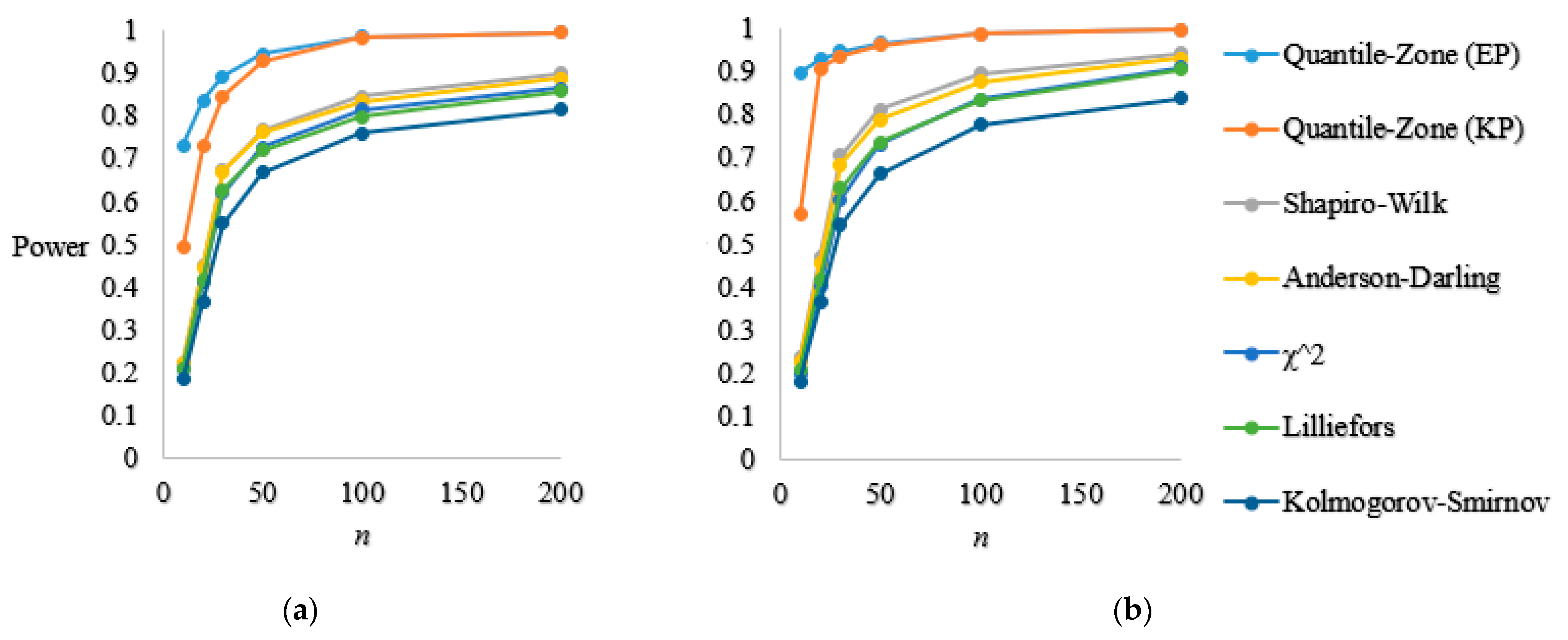
4. Comparative Analysis

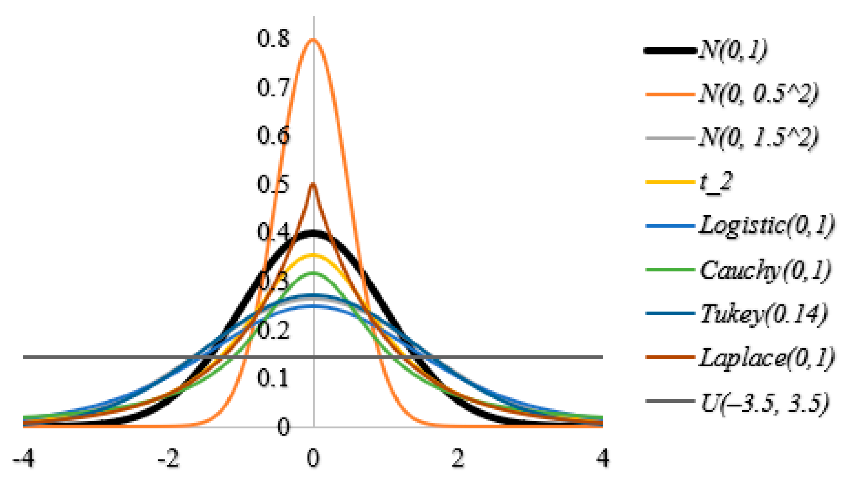
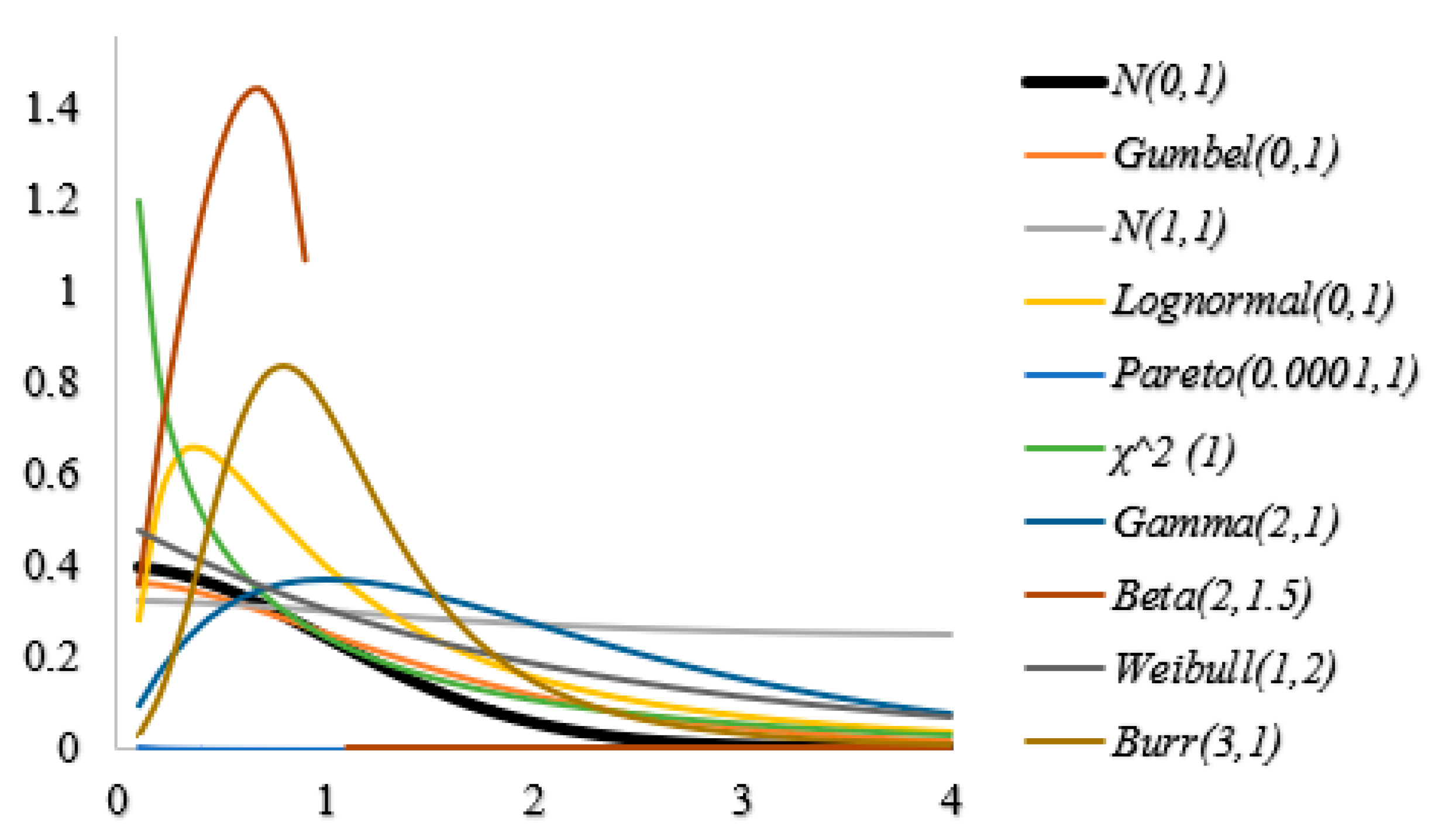
In this section, we compare the power values of our test to the most used normality tests. We provide average power values for various alternative distributions and sample sizes for mentioned tests and our Quantile-Zone test. Alternative distributions listed in Table 2 and Table 3 are the ones for which we calculated the average power values of our test.

The tests we compared our test to are: the Kolmogorov–Smirnov test [4] with its variant for estimated parameters (Lilliefors test) [5], Chi-square test [8], Shapiro–Wilk test [9] and Anderson–Darling test [7]. We discuss our test in both variants of given and estimated parameters.

We use the results for other tests approximated by the bisection method based on the ones obtained in [10]. Note that in [10], more alternative distributions were being used but were not separated. Instead, the authors provided the average power values. Additionally, we avoided using many alternative distributions that differ from the null distribution so that the histogram would be sufficient for a hypothesis rejection. That could cause an increase in power values for all the discussed tests, i.e., the results improved with big data [34]. If the identical alternative distributions were in use, the advantage of our test would be even better.

This way, we can see that though our results are not as thorough and precise (in [10], there were 1,000,000 simulations performed for every alternative distribution), they are still accurate and reliable enough.

We also note that the standard deviation of the power values is smaller than 0.3 for $n=10$ in all the exposed cases, for $n=30$ smaller than 0.2, and $n=200$ smaller than 0.01. Hence, in most cases, changing the alternative distribution will not have a significant effect on the variation of the average power value, especially considering the choice of the alternative distributions and rare exceptions where the empirical power is lower (see the second paragraph of Section 2.2 and the tables in Section 2.3—power analysis).

The following tables and figures show the results of the comparison.

As we can see, in both cases of estimated and known parameters, and symmetric and asymmetric alternative distributions, the Quantile-Zone test is the most powerful, even for $n=10$ (Table 7 and Table 8).

Table 7. Average empirical power values of statistic ${\overline{V}}_n$ and some other normality test statistics for various sample sizes with the level of significance $\mathit{\alpha }=0.05$—Symmetric alternative distributions.

Test	$\mathit{n}$
	10	20	30	50	100	200
Quantile-Zone (EP 1)	0.7309	0.8365	0.8945	0.9466	0.9855	0.9962
Quantile-Zone (KP 2)	0.4921	0.7294	0.8462	0.9295	0.9832	0.9962
Shapiro–Wilk	0.2244	0.4488	0.6732	0.7687	0.8452	0.8994
Anderson–Darling	0.2231	0.4462	0.6694	0.7618	0.8350	0.8889
${\mathit{\chi }}^{\mathbf{2}}$	0.2072	0.4144	0.6216	0.7277	0.8140	0.8657
Lilliefors	0.2091	0.4182	0.6272	0.7191	0.7974	0.8590
Kolmogorov–Smirnov	0.1828	0.3657	0.5485	0.6687	0.7602	0.8155

¹ Estimated parameters. ² Known parameters.

Table 8. Average empirical power values of statistic ${\overline{V}}_n$ and some other normality test statistics for various sample sizes with the level of significance $\alpha =0.05$—Asymmetric alternative distributions.

Test	$\mathit{n}$
	10	20	30	50	100	200
Quantile-Zone (EP 1)	0.8984	0.9294	0.9470	0.9664	0.9881	0.9978
Quantile-Zone (KP 2)	0.5673	0.9066	0.9367	0.9623	0.9878	0.9977
Shapiro–Wilk	0.2354	0.4707	0.7060	0.8127	0.8962	0.9442
Anderson–Darling	0.2279	0.4557	0.6835	0.7887	0.8761	0.9311
${\mathit{\chi }}^{\mathbf{2}}$	0.2016	0.4032	0.6047	0.7317	0.8364	0.9108
Lilliefors	0.2097	0.4194	0.6291	0.7357	0.8344	0.9041
Kolmogorov–Smirnov	0.1819	0.3638	0.5457	0.6627	0.7777	0.8398

¹ Estimated parameters. ² Known parameters.

For large samples ($n>200$), the Quantile-Zone test has the same power for both variants of known and estimated parameters.

The average powers for other tests are similar, therefore, choosing the right one could depend on the alternative distribution or the sample size only. In other words, other tests we mentioned could be considered equally powerful.

Therefore, the Quantile-Zone test is the best for normality testing in any circumstance.

All the figures and tables in the power analysis subsections, Table 7 and Table 8 and Figure 8, indicate no consistency issues in our test. Moreover, our test has better consistency properties than other most used tests since the slope of our test’s power function curve approximation is steeper than for the other tests (Figure 8). Even if that is not the case, higher average power values of our test would be the reason for surpassing the consistency issues.

Figure 8. Average empirical power values of statistic ${\overline{V}}_n$ and some other normality test statistics for various sample sizes with the level of significance $\alpha =0.05$: (a) Symmetric alternative distributions; (b) Asymmetric alternative distributions.

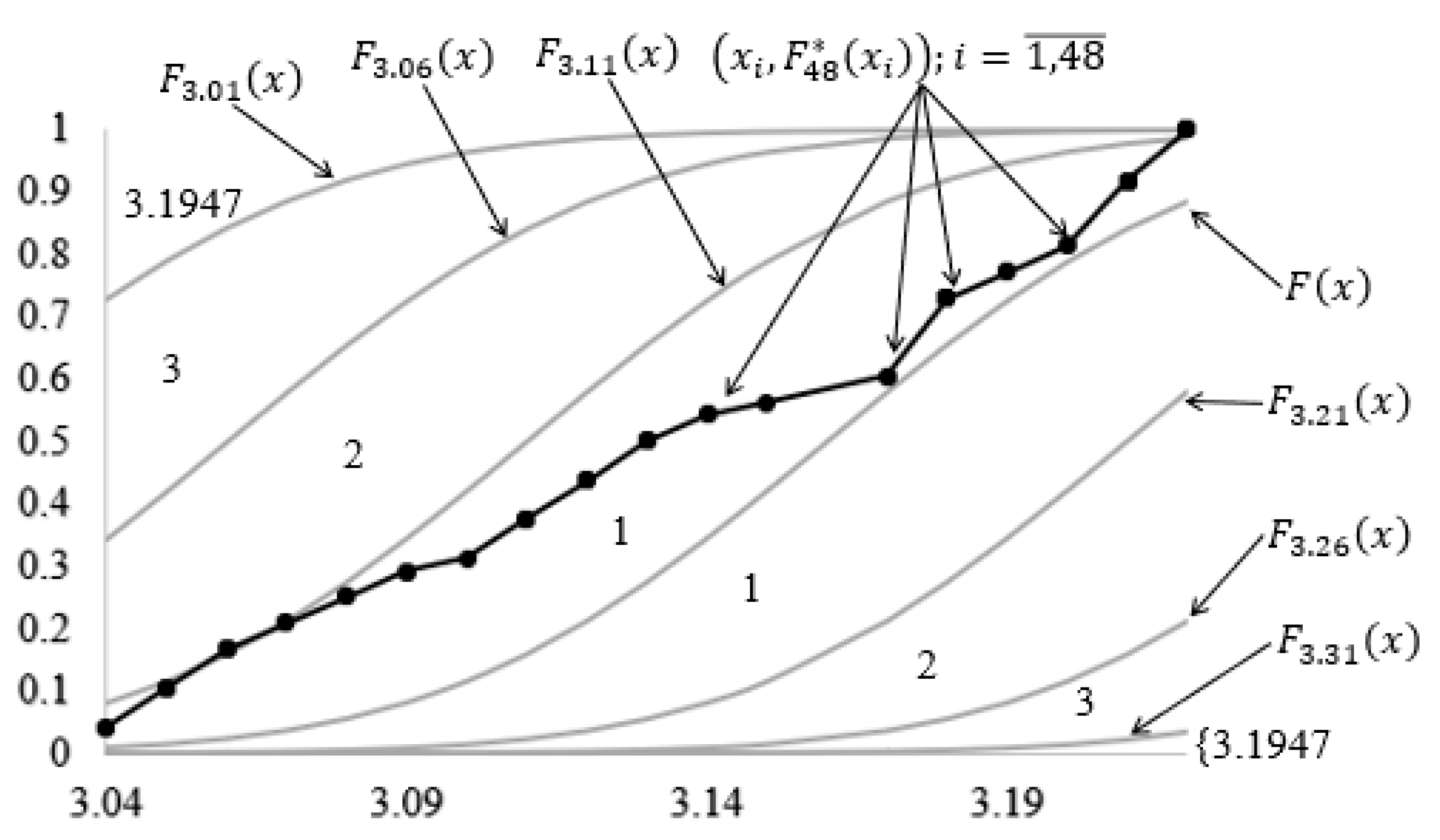
5. Real Data Example

To control the quantity of protein in milk, we take 48,100 g packages from the production line. Measurements have yielded the results: 3.04, 3.12, 3.12, 3.22, 3.09, 3.13, 3.21, 3.18, 3.10, 3.18, 3.21, 3.18, 3.04, 3.11, 3.17, 3.06, 3.13, 3.12, 3.11, 3.07, 3.15, 3.05, 3.14, 3.18, 3.11, 3.21, 3.22, 3.13, 3.06, 3.07, 3.17, 3.22, 3.05, 3.19, 3.18, 3.20, 3.08, 3.20, 3.21, 3.09, 3.05, 3.14, 3.22, 3.08, 3.19, 3.18, 3.21, 3.06 (in %). The concentration of the protein in milk is usually between three and four percent. We take two examples.

5.1. Known Parameters Case

We assume that the milk packages meet the standard if the protein concentration is distributed by the normal $N\left(3.15, {0.06}^2\right)$ distribution. We shall test this using the Quantile-Zone test.

Calculating the EDF of this sample and plotting the points $\left(x_i, F_{48}^{*}\left(x_i\right)\right); i=\overline{1, 48}$, we obtained the results shown in Figure 9.

Figure 9. Zones and points $\left(x_i, F_{48}^{*}\left(x_i\right)\right); i=\overline{1,48}$ for obtained data—Known parameters.

Using the results given in Figure 9 and Formula (2), we achieve ${\overline{v}}_{48}=1.2454$.

For the level of significance $\alpha =0.05$ the critical region is $W=\left[1,1.0013\right]\cup \left[1.0627,3.1947\right]$ (Table 1). Since ${\overline{v}}_{48}\in W$ we reject the null hypothesis, i.e., the protein concentration in milk is not distributed by the normal $N\left(3.16, {0.05}^2\right)$ distribution.

5.2. Estimated Parameters Case

We assume that the milk packages meet the standard if the protein concentration is distributed by the normal $N\left({\overline{x}}_{48}, {\tilde{s}}_{48}^2\right)~N\left(3.14, {0.06}^2\right)$ distribution. We shall test this using the Quantile-Zone test.

Calculating the EDF of this sample and plotting the points $\left(x_i, F_{48}^{*}\left(x_i\right)\right); i=\overline{1,48}$, we obtained the results shown in Figure 10.

Figure 10. Zones and points $\left(x_i, F_{48}^{*}\left(x_i\right)\right); i=\overline{1,48}$ for obtained data—Estimated parameters.

Using the results given in Figure 10 and Formula (2), we achieve ${\overline{v}}_{48}=1.1829$.

For the level of significance $\alpha =0.05$ the critical region is $W=\left[1,1.0013\right]\cup \left[1.0532,3.1947\right]$ (Table 4). Since ${\overline{v}}_{48}\in W$ we reject the null hypothesis, i.e., the protein concentration in milk is not distributed by the normal distribution.

Even though here the EDF is essentially located well, the normality of distribution is not confirmed. That is due to $n_{\max }=4$, i.e., 8.3% of the sample elements equals 3.22, which does not satisfy the basic normality properties.

6. Conclusions and Future Work

In this paper, we:

• Defined a new normality test statistic based on the “3-sigma” rule and basic properties of CDF and EDF;
• Provided some basic properties of the test statistic with its distribution tables for both cases of known and estimated parameters obtained through 100,000 Monte Carlo simulations;
• Elaborated on the choice of the two-tailed critical region;
• Elaborated on the advantage of our test statistics when it comes to outliers and the simplicity of implementation;
• Provided detailed power analysis for various sample sizes and symmetric and asymmetric alternative distribution for the level of significance of 0.05;
• Discussed both cases of known and estimated parameters of the null distribution as well as the power calculating process through 10,000 Monte Carlo simulations;
• Performed comparative analysis of our test power performance and the other most used normality tests and thus proved that our test is the best choice when testing normality;
• Provided tabular and graphical representations of all the results.

The future work will consist of researching some additional properties of the test statistic and, if possible, functional characteristics of its distribution. If it turns out as needed, more detailed power analysis and comparative analyses are possibilities.

Other ideas are expanding the Quantile-Zone approach to the general goodness-of-fit testing and some new approaches to the same problem. We are also considering the possibility of extending this solution principle to multivariate normality testing.

References

- Thode, H.C., Jr. Testing for Normality; Marcel Dekker AG: Basel, Switzerland, 2002. [Google Scholar]
- Hogg, R.V.; McKean, J.W.; Craig, A.T. Introduction to Mathematical Statistics, 8th ed.; Pearson Education, Inc.: Boston, MA, USA, 2019. [Google Scholar]
- Öztürk, A.; Dudewicz, E.J. A New Statistical Goodness-of-Fit Test Based on Graphical Representation. Biom. J. 1995, 34, 403–427. Available online: https://ur.booksc.eu/book/684213/e0fa15 (accessed on 27 April 2022). [CrossRef]
- Massey, F.J., Jr. The Kolmogorov-Smirnov Test for Goodness of Fit. J. Am. Stat. Assoc. 1951, 46, 68–78. [Google Scholar] [CrossRef]
- Lilliefors, H.W. On the Kolmogorov-Smirnov Test for Normality with Mean and Variance Unknown. J. Am. Stat. Assoc. 1967, 62, 399–402. [Google Scholar] [CrossRef]
- Anderson, T.W.; Darling, D.A. Asymptotic Theory of Certain “Goodness of Fit” Criteria Based on Stochastic Processes. Ann. Math. Stat. 1952, 23, 193–212. Available online: http://www.jstor.org/stable/2236446 (accessed on 27 April 2022). [CrossRef]
- Anderson, T.W.; Darling, D.A. A Test of Goodness of Fit. J. Am. Stat. Assoc. 1954, 49, 765–769. [Google Scholar] [CrossRef]
- Cochran, W.G. The χ2 Test of Goodness of Fit. Ann. Math. Stat. 1952, 23, 315–345. Available online: http://www.jstor.org/stable/2236678 (accessed on 27 April 2022). [CrossRef]
- Shapiro, S.S.; Wilk, M.B. An analysis of variance test for normality (complete samples). Biometrika 1965, 52, 591–611. [Google Scholar] [CrossRef]
- Arnastauskaitė, J.; Ruzgas, T.; Bražėnas, M. An Exhaustive Power Comparison of Normality Tests. Mathematics 2021, 9, 788. [Google Scholar] [CrossRef]
- Sürücü, B. A power comparison and simulation study of goodness-of-fit tests, Computers and Mathematics with applications. Elsevier 2008, 56, 1617–1625. [Google Scholar] [CrossRef] [Green Version]
- Slakter, M.J. A Comparison of the Pearson Chi-Square and Kolmogorov Goodness-of-Fit Tests with Respect to Validity. J. Am. Stat. Assoc. 1965, 60, 854–858. [Google Scholar] [CrossRef]
- Noughabi, H.A. A Comprehensive Study on Power of Tests for Normality. J. Stat. Theory Appl. 2018, 17, 647–660. [Google Scholar] [CrossRef]
- Razali, N.M.; Wah, Y.B. Power Comparisons of Shapiro-Wilk, Kolmogorov-Smirnov, Lilliefors and Ander-son-Darling Tests. J. Stat. Model. Anal. 2011, 2, 21–33. Available online: https://www.researchgate.net/publication/267205556_Power_Comparisons_of_Shapiro-Wilk_Kolmogorov-Smirnov_Lilliefors_and_Anderson-Darling_Tests (accessed on 27 April 2022).
- Ahmad, F.; Khan, R.A. A power comparison of various normality tests. Pak. J. Stat. Oper. Res. 2015, 11, 331–345. [Google Scholar] [CrossRef] [Green Version]
- Boyerinas, B.M. Determining the Statistical Power of the Kolmogorov-Smirnov and Anderson-Darling Goodness-of-Fit Tests via Monte Carlo Simulation. CNA Analysis and Solutions. 2016. Available online: https://www.cna.org/CNA_files/PDF/DOP-2016-U-014638-Final.pdf (accessed on 27 April 2022).
- Kanji, G.K. 100 Statistical Tests; SAGE Publications: London, UK, 2006. [Google Scholar]
- Tucker, H.G. A Generalization of the Glivenko-Cantelli Theorem. Ann. Math. Stat. 1959, 30, 828–830. Available online: https://www.jstor.org/stable/2237422 (accessed on 5 April 2020). [CrossRef]
- Law of Large Numbers. Encyclopedia of Mathematics. Available online: http://encyclopediaofmath.org/index.php?title=Law\_of\_large\_numbers\&oldid=47595 (accessed on 27 April 2022).
- Ritter, F.E.; Schoelles, M.J.; Quigley, K.S.; Klein, L.C. Determining the Number of Simulation Runs: Treating Simulations as Theories by Not Sampling Their Behavior. In Human-in-the-Loop Simulations; Springer: London, UK, 2011. [Google Scholar]
- Gentle, J.E. Random Numbers Generation and Monte Carlo Methods, 2nd ed.; George Mason University: Fairfax, VA, USA, 2002. [Google Scholar]
- Rubenstein, R.Y. Simulation and the Monte Carlo Method; John Wiley and Sons: New York, NY, USA, 1981. [Google Scholar]
- Jevremović, V.; Avdović, A. Control Charts Based on Quantiles—New Approaches. Scientific Publications of the State University of Novi Pazar, Series A, Applied Mathematics. Inform. Mech. 2020, 12, 99–104. [Google Scholar] [CrossRef]
- Jevremović, V.; Avdović, A. Empirical Distribution Function as a Tool in Quality Control. Scientific Publications of the State University of Novi Pazar, Series A, Applied Mathematics. Inform. Mech. 2020, 12, 37–46. [Google Scholar] [CrossRef]
- Oakland, J.S. Statistical Process Control; Butterworth-Heinman: Oxford, UK, 2003. [Google Scholar]
- Bakir, S.T. A Nonparametric Shewhart-Type Quality Control Chart for Monitoring Broad Changes in a Process Distribution. J. Qual. Reliab. Eng. 2012, 2012, 147520. [Google Scholar] [CrossRef]
- Arnastauskaitė, J.; Ruzgas, T.; Bražėnas, M. A New Goodness of Fit Test for Multivariate Normality and Comparative Simulation Study. Mathematics 2021, 9, 3003. [Google Scholar] [CrossRef]
- Elbouch, S.; Michel, O.; Comon, P. A Normality Test for Multivariate Dependent Samples. HAL. 2022. Available online: https://hal.archives-ouvertes.fr/hal-03344745 (accessed on 27 April 2022).
- Song, Y.; Zhao, X. Normality Testing of High-Dimensional Data Based on Principle Component and Jarque–Bera Statistics. Stats 2021, 4, 16. [Google Scholar] [CrossRef]
- Opheim, T.; Roy, A. More on the Supremum Statistic to Test Multivariate Skew-Normality. Computation 2021, 9, 126. [Google Scholar] [CrossRef]
- Đorić, D.; Jevremović, V.; Mališić, J.; Nikolić-Đorić, E. Atlas of Distributions; Faculty of Civil Engineering: Belgrade, Serbia, 2007. (In Serbian) [Google Scholar]
- MATLAB Help Center. Creating and Controlling a Random Number Stream. Available online: https://www.mathworks.com/help/matlab/math/creating-and-controlling-a-random-number-stream.html (accessed on 27 April 2022).
- Dwivedi, A.K.; Mallawaarachchi, I.; Alvarado, L.A. Analysis of small sample size studies using nonparametric bootstrap test with pooled resampling method. Stat. Med. 2017, 36, 2187–2205. [Google Scholar] [CrossRef] [PubMed]
- Klimek, K.M. Analiza mocy testu i liczebności próby oraz ich znaczenie w badaniach empirycznych. Wiad. Lek. 2008, 61, 211–215. [Google Scholar] [PubMed]
Publisher’s Note: MDPI stays neutral with regard to jurisdictional claims in published maps and institutional affiliations. |
© 2022 by the authors. Licensee MDPI, Basel, Switzerland. This article is an open access article distributed under the terms and conditions of the Creative Commons Attribution (CC BY) license (https://creativecommons.org/licenses/by/4.0/).