On Resolvability- and Domination-Related Parameters of Complete Multipartite Graphs

Abstract

Graphs of order n with fault-tolerant metric dimension n have recently been characterized.This paper points out an error in the proof of this characterization. We show that the complete multipartite graphs also have the fault-tolerant metric dimension n, which provides an infinite family of counterexamples to the characterization. Furthermore, we find exact values of the metric, edge metric, mixed-metric dimensions, the domination number, locating-dominating number, and metric-locating-dominating number for the complete multipartite graphs. These results generalize various results in the literature from complete bipartite to complete multipartite graphs.

1. Introduction

This paper takes only finite, connected and simple graphs into account. The reader is referred to Section 2 for undefined notations and terminologies.

The concept of metric dimension was first defined independently by Slater in 1975 [1], and later, it was discussed in 1976 by Harary and Melter [2]. It has been studied widely since then. Metric dimension has diverse applications in fields such as graph theory [3,4], robot navigation [5], chemistry [6], telecommunication networks [7], combinatorial optimization [8], geographical routing protocols [9], sociology [10] and many more.

The metric dimension has been studied extensively since it has been introduced. For instance, in [11,12,13,14,15,16,17,18,19,20,21], the authors studied the metric dimension of certain infinite families of graphs. Other variants of metric dimension such as the edge metric and the mixed-metric dimension of graphs have been defined by Kelenc et al. [22] and Kelenc et al. [23], respectively. The edge metric dimension for various families of graphs has been studied in [24,25,26,27], among others. The mixed metric dimension for various families of graphs has been investigated in [28,29,30], among others. The fault-tolerant metric dimension of graphs has been introduced by Hernando et al. [31] back in 2008 as a natural extension of the metric dimension. The reader is referred to [32,33,34,35] for various mathematical properties of fault-tolerant resolvability in graphs.

We refer the interested readers to the book by Henning et al. [36], which provides, until 1980, a brief overview of the results regarding domination in graphs. Haynes et al. [37] considered trees for their total domination and the binary location-domination numbers. Minimum ℓ-locating-dominating as well as ℓ-identifying sets/representations in chains and cyclic graphs have been constructed by Charon et al. [38]. Sharp upper and lower bounds on the minimality of ℓ-locating-dominating sets for general graph were also found. For further reading on these contemporary domination-related parameters, we refer to [39,40].

Salter [41] and Seo et al. [42,43] introduced the concepts of the open-neighborhood location-domination number and the fault-tolerant location-domination number, respectively, and found results on these parameters for trees. The location-domination number for certain classes of convex polytopes was investigated recently by Raza et al. [8] and Simić et al. [44]. They found its exact values for some families of convex polytopes and tight upper bounds were found for other families. The reader is suggested to read [40,45,46,47] for more details on these domination-related graph-theoretic parameters. Generalized Petersen graphs are of prime importance in graph theory and they provide counterexamples to many graph-theoretic conjectures. They were considered by a number of researchers in [48,49,50,51,52] for their parameters related to domination in graphs.

Taking the extensive literature on the resolvability- and domination-related parameters of graphs into account, in this paper, we find exact values of the metric, edge metric, fault-tolerant metric, and mixed metric dimensions of complete multipartite graphs. We also compute the domination number, locating-dominating number, and the metric-locating-dominating number of the complete multipartite graphs. In particular, we show that the fault-tolerant metric dimension of n-vertex complete multipartite graphs is n. This, in turn, provides an infinite family of counterexamples to Theorem 7 [53] by Raza et al., who showed that the complete graphs are the only graphs with fault-tolerant metric dimension n. Section 3.2 points out an error in the proof of Theorem 7 [53] by Raza et al. Other results generalize various results in the literature from complete bipartite to complete multipartite graphs.

2. Preliminaries

A graph is an ordered pair $\mathsf{\Gamma }(V_{\mathsf{\Gamma }},E_{\mathsf{\Gamma }})$, where $V_{\mathsf{\Gamma }}$ denotes the point/vertex set and $E_{\mathsf{\Gamma }}$ the line/edge set. Let the non-adjacency (resp. adjacency) of a pair of vertices $y,z\in V_{\mathsf{\Gamma }}$ be denoted by $y\nsim z$ (resp. $y\sim z$), implying that $yz\notin E_{\mathsf{\Gamma }}$ (resp. $yz\in E_{\mathsf{\Gamma }}$). A graph $\mathsf{\Gamma }(V_{\mathsf{\Gamma }},E_{\mathsf{\Gamma }})$ is said to be finite if $V_{\mathsf{\Gamma }}$ is a finite set. An edge is called a loop if its end-vertices are the same. Two edges are said to be multiedges if they have the same end-vertices. For $y\in V_{\mathsf{\Gamma }}$, the open (resp. close) neighborhood of y is $\mathcal{N}\left(y\right)=\{z\in V_{\mathsf{\Gamma }}\mid yz\in E_{\mathsf{\Gamma }}\}$ (resp. $\mathcal{N}\left[y\right]=\left\{y\right\}\cup \{z\in V_{\mathsf{\Gamma }}\mid yz\in E_{\mathsf{\Gamma }}\}$). The number $\mid \mathcal{N}\left(y\right)\mid :={\mathrm{deg}}_{\mathsf{\Gamma }}\left(y\right)$ is known to be the degree of y. Contextual understanding of $\mathsf{\Gamma }$ in the text tends to omit $\mathsf{\Gamma }$ from notations $V_{\mathsf{\Gamma }}$, ${\mathrm{deg}}_{\mathsf{\Gamma }}\left(y\right)$ and $E_{\mathsf{\Gamma }}$. A graph is said to be connected if every pair of vertices are connected by a path. It is called undirected if none of its edges has some orientation. Therefore, the binary relation on vertices ‘being adjacent’ in an undirected graph is symmetric. A graph is said to be simple if it has no loops or multiedges.

A complete graph $K_n$ is an n-vertex graph whose vertices are pairwise adjacent. An independent set $I\subset V_{\mathsf{\Gamma }}$ in a graph $\mathsf{\Gamma }$, is a set of mutually disjoint non-adjacent vertices in $\mathsf{\Gamma }$. A r-partite graph is a graph whose vertices are or can be partitioned into r different independent sets. A complete r-partite graph is an r-partite graph in which there is an edge between every pair of vertices from different independent sets. A complete r-partite graph is usually denoted by $K_{t_1,t_2,\dots ,t_r}$. Let $T_r$ be the $r^{\mathrm{th}}$ partite set of $K_{t_1,t_2,\dots ,t_r}$ such that $t_i:=\mid T_i\mid$ ($1\le i\le r$). Thus, alternatively, a complete r-partite graph is an r-partite graph such that $\forall x\in T_i,\exists j\ne i,\exists y\in T_j,xy\in E_{\mathsf{\Gamma }}$ is satisfied. Note that if $t_i=1$ for $1\le i\le r$, then $K_{t_1,t_2,\dots ,t_r}=K_n$ such that ${\displaystyle \sum _{i=1}^r}{t}_i=n$. Thus, if we consider non-complete graphs, then we may assume that $1\le t_1\le t_2\le \dots \le t_r$ such that $t_1\ge 1$ and $t_i\ge 2$ for $2\le i\le r$. For more notations and terminologies, we refer the book on molecular topology by Diudea et al. [54]. Note that simple graphs have important connection with mathematical chemistry, as described by Joiţa and Jäntschi [55]. More rich literature on mathematical chemistry and chemical graph theory can be found in [56,57].

The length of the shortest path between a pair $y,z\in V_{\mathsf{\Gamma }}$ is said to be the distance $d(y,z)$ between them. Let $Y={\left\{y_k\right\}}_{k=1}^{\ell }\subseteq V\left(\mathsf{\Gamma }\right)$ and $x\in V\left(\mathsf{\Gamma }\right)$. The distance representation $r_Y\left(x\right)$ is the vector $\left(d(x,y_1)\dots ,d(x,y_{\ell })\right)$ of distances from x to $y_k(1\le k\le \ell )$. If all vertices of $\mathsf{\Gamma }$ have distinct distance representations corresponding to Y, the set Y is said to be a resolving set. The metric dimension $\beta \left(\mathsf{\Gamma }\right)$ (or simply md) is the smallest cardinality of such a resolving set in $\mathsf{\Gamma }$ [1]. A resolving set of cardinality $\beta \left(\mathsf{\Gamma }\right)$ in $\mathsf{\Gamma }$ is said to be a metric generator of $\mathsf{\Gamma }$.

In order to explain the concept of a resolving set, let us take the example of the well-known Petersen graph P, see Figure 1. The set $S=\{v_1,v_2,u_3,u_4\}$ is a resolving set of P, since all distance representations of vertices in $V\left(P\right)\setminus S$, i.e.,

$$\begin{array}{ccc}\hfill r_S\left(u_1\right)=(1,2,2,2);& & r_S\left(u_2\right)=(2,1,1,2);\hfill \\ \hfill r_S\left(u_5\right)=(2,2,2,1);& & r_S\left(v_3\right)=(1,2,1,2);\hfill \\ \hfill r_S\left(v_4\right)=(1,1,2,1);& & r_S\left(v_5\right)=(2,1,2,2),\hfill \end{array}$$

are all unique. However, if you observe the distance representations, then we can see that removing the last component from each vector would also keep the representations unique. This implies that the set $R=S\setminus \left\{u_4\right\}$ is also a resolving set. It can be shown that there exists no resolving set of cardinality 2 in P. Thus, $\beta \left(P\right)=3.$

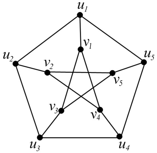
Figure 1. The Petersen graph P.

Let Y be a resolving set. If $Y^{\prime }=Y\setminus \left\{y\right\}$ is also a resolving set for any $y\in Y$, then Y is called a fault-tolerant resolving set of $\mathsf{\Gamma }$. Symbolized as ${\beta }^{\prime }\left(\mathsf{\Gamma }\right)$, the fault-tolerant metric dimension (or ftmd) [31] of $\mathsf{\Gamma }$ is the smallest cardinality of such kind of resolving set of $\mathsf{\Gamma }$. A fault-tolerant resolving set of cardinality ${\beta }^{\prime }\left(\mathsf{\Gamma }\right)$ in $\mathsf{\Gamma }$ is said to be a fault-tolerant metric generator of $\mathsf{\Gamma }$. See more on distances in graphs in a book on this title by Buckley and Harary [3].

The tree T in Figure 2 has $\beta \left(T\right)=10$ and ${\beta }^{\prime }\left(T\right)=14$. The set $P=(1,2,3,4,\dots ,10)$ (resp. $Q=P\cup \{y,v,r,s\}$) forms the metric generator (resp. fault-tolerant metric generator) of T.

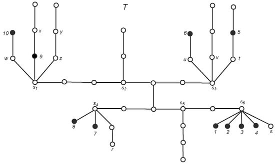
Figure 2. The tree example T with $\beta \left(T\right)=10$ and ${\beta }^{\prime }\left(T\right)=14$.

For $y\in V_{\mathsf{\Gamma }}$ and $f=ab\in E_{\mathsf{\Gamma }}$, the vertex-edge metric/distance is determined as $d(y,f):=min\left\{d\right(a,y),d(b,y\left)\right\}$. A vertex $y\in V_{\mathsf{\Gamma }}$ is known to resolve two edges $f,g\in E\left(\mathsf{\Gamma }\right)$ if we have $d(y,f)\ne d(y,g)$. An edge-resolving set is a set $Y={\left\{y_k\right\}}_{k=1}^{\ell }\subseteq V_{\mathsf{\Gamma }}$ if all pairwise edges are resolved by some $y_k\in Y(1\le k\le \ell )$. Symbolized as ${\beta }_e\left(\mathsf{\Gamma }\right)$, the edge metric dimension (or emd) [22] is the smallest cardinality of such a resolving set of $\mathsf{\Gamma }$. An edge resolving set of cardinality ${\beta }_e\left(\mathsf{\Gamma }\right)$ in $\mathsf{\Gamma }$ is said to be an edge metric generator of $\mathsf{\Gamma }$. On the other hand, a vertex $w\in V_{\mathsf{\Gamma }}$ is known to resolve $y,z\in V\cup E$ if $d(w,y)\ne d(w,z)$ is satisfied. A mixed-resolving set is a subset $Y={\left\{y_k\right\}}_{k=1}^{\ell }\subseteq V\left(\mathsf{\Gamma }\right)$ for which a pair of two elements of $V\cup E$ is resolved by some vertex of Y. Minimum cardinality ${\beta }_m\left(\mathsf{\Gamma }\right)$ of such a mixed-resolving set is known as the mixed-metric dimension (or mmd) [23] of $\mathsf{\Gamma }$. A mixed resolving set of cardinality ${\beta }_m\left(\mathsf{\Gamma }\right)$ in $\mathsf{\Gamma }$ is said to be a mixed metric generator of $\mathsf{\Gamma }$.

From the definition of an edge resolving set, we obtain that:

$${\beta }_m\left(\mathsf{\Gamma }\right)\ge max\{\beta \left(\mathsf{\Gamma }\right),{\beta }_e\left(\mathsf{\Gamma }\right)\}.$$

(1)

A vertex $z\in \mathcal{N}\left(y\right)$ for an arbitrary $y\in V_{\mathsf{\Gamma }}$ is known as a maximal neighbor of y, if $\mathcal{N}\left[y\right]\subseteq \mathcal{N}\left[z\right]$. Kelenc et al. [23] proved a result as follows:

Theorem 1.

[23] For an n-vertex graph Γ, we have ${\beta }_m\left(\mathsf{\Gamma }\right)=n$ if and only if every vertex of Γ has a maximal neighbor.

A set $L\subset V_{\mathsf{\Gamma }}$ satisfying $L\cap \mathcal{N}\left(y\right)\ne \varnothing$ for every $y\in V_{\mathsf{\Gamma }}\setminus L$ is known to dominate (i.e., a dominating set of) $\mathsf{\Gamma }$. The smallest cardinality $\gamma \left(\mathsf{\Gamma }\right)$ of such a dominating set is known to be the domination number of $\mathsf{\Gamma }$. A dominating generator is simply a dominating set having cardinality $\gamma \left(\mathsf{\Gamma }\right)$. For $T\subset V_{\mathsf{\Gamma }}$, a vertex $y\in V_{\mathsf{\Gamma }}$ is known to dominate T if $T\subseteq \mathcal{N}\left(y\right)$. If, in addition to being a dominating set, a set L has distinct distance representation respective to vertices in L, it is known as a metric-locating-dominating (mld) set. Smallest cardinality ${\gamma }_{mld}\left(\mathsf{\Gamma }\right)$ of an mld set is known to be the metric-location-domination number (mldn) [41]. Note that an mld set is both a resolving and a dominating set. Therefore, the mld number creates an interconnection between resolvability and domination in graph. See the book by Henning et al. [36] for more on the domination theory of graphs.

An alternative way of investigating a dominating set is by allocating 1 (resp. 0) to $y\in L$ (resp. $y\in V_{\mathsf{\Gamma }}\setminus L$). Given this, L is a dominating set of $\mathsf{\Gamma }$ if for any $y\in V_{\mathsf{\Gamma }}$ the sum of weights for closed neighborhoods is at least 1, i.e., $\mid \mathcal{N}\left[x\right]\cap L\mid \ge 1$. For L being a dominating set, if in addition, it holds $\mathcal{N}\left(y\right)\cap L\ne \mathcal{N}\left(z\right)\cap L$ for any pair $y,z\in V_{\mathsf{\Gamma }}\setminus L$, we call L a locating-dominating (LD) set. The smallest cardinality of such an LD set is symbolized as ${\gamma }_{l-d}\left(\mathsf{\Gamma }\right)$ and known as the LD number of $\mathsf{\Gamma }$. An LD generator is an LD set of cardinality ${\gamma }_{l-d}\left(\mathsf{\Gamma }\right)$. Note that we have $\gamma \left(\mathsf{\Gamma }\right)\le {\gamma }_{l-d}\left(\mathsf{\Gamma }\right)$.

Next, the main results of this paper have been shown.

3. Resolvability-Related Parameters

This first section computes certain resolvability parameters, such as the metric dimension, the fault-tolerant metric dimension, the edge metric dimension, and the mixed metric dimension of complete multipartite graphs.

3.1. Metric Dimension

This section computes the metric dimension of complete multipartite graphs.

Theorem 2.

Let $K_{t_1,t_2,\dots ,t_r}$ be the complete r-partite graph with $1\le t_1\le t_2\le \dots \le t_r$ and ${\displaystyle \sum _{i=1}^r}{t}_i=n$. Then:

$$\beta \left(K_{t_1,t_2,\dots ,t_r}\right)=\sum _{i=1}^r{t}_i-r=n-r.$$

(2)

Proof. 

First, we show the following two claims.

Claim 1.

If $r=2$, then $\beta \left(K_{t_1,t_2}\right)=t_1+t_2-2$.

Proof of Claim 1.

Assume $T_1$ and $T_2$ are partite sets of $K_{t_1,t_2}$, having $\mid T_1\mid =t_1$ and $\mid T_2\mid =t_2$. For any $y\in T_1$ and $z\in T_2$, we assume $S=T_1\cup T_2\setminus \{y,z\}$. Note that S is a resolving set of $K_{t_1,t_2}$, since $r_S\left(y\right)=(\underset{t_1-1\mathrm{times}}{\underbrace{2,2,\dots ,2}},\underset{t_2-1\mathrm{times}}{\underbrace{1,1,\dots ,1}})$ and $r_S\left(z\right)=(\underset{t_1-1\mathrm{times}}{\underbrace{1,1,\dots ,1}},\underset{t_2-1\mathrm{times}}{\underbrace{2,2,\dots ,2}})$. Since $r_S\left(y\right)\ne r_S\left(z\right)$, therefore, S is a resolving set. This implies that $\beta \le \mid S\mid =t_1+t_2-2$.

On the other hand, let $x\in S$ such that $x\notin \{y,z\}$. Let $S^{\prime }=T_1\cup T_2\setminus \{x,y,z\}$. Assume, without loss of generality, that $x\in T_2$. Then $r_{S^{\prime }}\left(z\right)=r_{S^{\prime }}\left(x\right)=(\underset{t_1-1\mathrm{times}}{\underbrace{1,1,\dots ,1}},\underset{t_2-2\mathrm{times}}{\underbrace{2,2,\dots ,2}})$. Since x was arbitrary and $S^{\prime }$ is not a resolving set, we obtain that x must belong to $S^{\prime }$. This implies that there is no resolving set of cardinality $t_1+t_2-3$ in $K_{t_1,t_2}$, and thus, we have $\beta \left(K_{t_1,t_2}\right)\ge t_1+t_2-2$. This complete the proof. □

Claim 2.

If $r=3$, then $\beta \left(K_{t_1,t_2,t_3}\right)=t_1+t_2+t_3-2$.

Proof of Claim 2.

Let $T_1,T_2$ and $T_3$ be three partite sets such that $|T_1|=t_1$ and $|T_2|=t_2$ and $|T_3|=t_3$. Assume that $R=T_1\cup T_2\cup T_3\setminus \{x,y,z\}$, for arbitrary $x\in T_1$, $y\in T_2$ and $z\in T_3$. Note that R is a resolving set as $r_R\left(x\right)\ne r_R\left(y\right)\ne r_R\left(z\right)$, where $r_R\left(x\right)=(\underset{t_1-1\mathrm{times}}{\underbrace{2,\dots ,2}},\underset{t_2-1\mathrm{times}}{\underbrace{1,\dots ,1}},\underset{t_3-1\mathrm{times}}{\underbrace{1,\dots ,1}})$, $r_R\left(y\right)$$=(\underset{t_1-1\mathrm{times}}{\underbrace{1,\dots ,1}},\underset{t_2-1\mathrm{times}}{\underbrace{2,\dots ,2}},\underset{t_3-1\mathrm{times}}{\underbrace{1,\dots ,1}})$ and $r_R\left(y\right)$$=(\underset{t_1-1\mathrm{times}}{\underbrace{1,\dots ,1}},\underset{t_2-1\mathrm{times}}{\underbrace{1,\dots ,1}},\underset{t_3-1\mathrm{times}}{\underbrace{2,\dots ,2}})$. Thus, we have $\beta \le \left|R\right|=t_1+t_2+t_3-3$.

For arbitrary vertex $w\in R$ where $w\notin \{x,y,z\}$, let $R^{\prime }=T_1\cup T_2\cup T_3\setminus \{w,x,y,z\}$. Without loss of generality, we assume that $w\in T_1$, then $r_{R^{\prime }}\left(x\right)=r_{R^{\prime }}\left(w\right)=(\underset{t_1-2\mathrm{times}}{\underbrace{2,\dots ,2}},\underset{t_2-1\mathrm{times}}{\underbrace{1,\dots ,1}},\underset{t_3-1\mathrm{times}}{\underbrace{1,\dots ,1}})$. This shows that $R^{\prime }$ is not a resolving set. Since w was arbitrary, we see that there is no resolving set of cardinality $t_1+t_2+t_3-4$. This implies that $\beta \left(K_{t_1,t_2,t_3}\right)\ge t_1+t_2+t_3-3$. Combining both inequalities, we obtain the result. □

For general r, we apply induction on r. By Claims 3.1 and 3.1, the result is true for $r=2$ and $r=3$, respectively. For the induction step, assume that (2) holds for $r=k$. Now, we show that this is true for $r=k+1$.

Let $T_i$ ($1\le i\le r$) be the $i^{\mathrm{th}}$ partite set with $|T_i|=t_i$. Since Equation (2) holds for $r=k$, we obtain that:

$$\beta \left(K_{t_1,t_2,\dots ,t_k}\right)=\sum _{i=1}^k{t}_i-k,$$

and that there exists a minimum resolving set R with $\mid R\mid ={\displaystyle \sum _{i=1}^k}{t}_i-k$. Note that R must contain $t_i-1$ vertices from $T_i$ for every $1\le i\le k$; otherwise, if R would contain two vertices from the same partite set, then they would have the same distance representations. Furthermore, this would contradict the fact that R is a resolving set. For $i=1,\dots ,k$, let $T_i\setminus R=\left\{x_i\right\}$ such that $V\left(K_{t_1,t_2,\dots ,t_k}\right)\setminus R=\{x_1,\dots ,x_k\}$. Note that for every $i=1,\dots ,k$, we have:

$$\begin{array}{ccc}\hfill r_R\left(x_i\right)& =& (c_1,c_2,\dots ,c_i,\dots ,c_k)\mathrm{where}\hfill \\ \hfill c_j& =& (\underset{t_j-1\mathrm{times}}{\underbrace{1,1,\dots ,1}})\mathrm{for}i\ne j=1,\dots ,k\mathrm{and}\hfill \\ \hfill c_i& =& (\underset{t_i-1\mathrm{times}}{\underbrace{2,2,\dots ,2}}).\hfill \end{array}$$

(3)

Clearly, $r_R\left(x_i\right)\ne r_R\left(x_j\right)$, where $1\le i,j\le k$ and $i\ne j$.

Now by adding $(k+1)\mathrm{th}$ partite set, say, $T_{k+1}$ to $K_{t_1,\dots ,t_k}$, we obtain $K_{t_1,\dots ,t_k,t_{k+1}}$. Let $R^{\prime }$ be the union of R and any of the $t_{k+1}-1$ vertices of $T_{k+1}$. Assume that $T_{k+1}\setminus R^{\prime }=\left\{x_{k+1}\right\}$. Then, we have $r_{R^{\prime }}\left(x_i\right)=(c_1,c_2,\dots ,c_i,\dots ,c_k,c_{k+1})$, where $c_j=(\underset{t_j-1\mathrm{times}}{\underbrace{1,1,\dots ,1}})$ for $i\ne j=1,\dots ,k+1$ and $c_i=(\underset{t_i-1\mathrm{times}}{\underbrace{2,2,\dots ,2}})$. Then, with (3), we obtain that $r_{R^{\prime }}\left(x_i\right)\ne r_{R^{\prime }}\left(x_j\right)$, where $1\le i,j\le k+1$ and $i\ne j$. This shows that $R^{\prime }$ is a resolving set and its minimum since R is minimum. Thus:

$$\beta \left(K_{t_1,t_2,\dots ,t_{k+1}}\right)=\sum _{i=1}^{k+1}{t}_i-(k+1).$$

By the induction hypothesis, the proof is finished. □

The following example illustrates an application of Theorem 2.

Example 1.

Let $K_{2,3,5}$ be the complete multipartite graph as depicted in Figure 3. Then, its seven black vertices form a metric generator. By Theorem 2, we obtain that $\beta \left(K_{2,3,5}\right)=10-3=7$.

Figure 3. The complete multipartite graph $K_{2,3,5}$ with a metric generator (black vertices).

It is important to remark the following:

Remark 1.

Note that Theorem 2 generalizes a result of Saputro et al. [58], who computed bounds on the metric dimension of complete multipartite graphs.

3.2. Fault-Tolerant Metric Dimension

In Theorem 7 [53], Raza et al. characterized n-vertex graphs with ${\beta }^{\prime }\left(\mathsf{\Gamma }\right)=n$. In particular, they showed the complete graphs are the only graphs satisfying ${\beta }^{\prime }\left(\mathsf{\Gamma }\right)=n$. They used the classification of n-ordered graphs with $\beta \left(\mathsf{\Gamma }\right)=n-1$, together with

$${\beta }^{\prime }\left(\mathsf{\Gamma }\right)\ge \beta \left(\mathsf{\Gamma }\right)+1,$$

(4)

to show Theorem 7 [53]. However, relationship in $\beta \left(\mathsf{\Gamma }\right)\le n-1$ does not ensure a relationship in (4). This fact makes the proof of Theorem 7 [53] invalid.

The next theorem proves that the complete multipartite graphs has ${\beta }^{\prime }\left(\mathsf{\Gamma }\right)=n$, and thus, providing an infinite family of counterexamples to Theorem 7 [53].

Theorem 3.

Let $K_{t_1,t_2,\dots ,t_r}$ be the complete r-partite graph with $1\le t_1\le t_2\le \dots \le t_r$ and ${\displaystyle \sum _{i=1}^r}{t}_i=n$. Then:

$${\beta }^{\prime }\left(K_{t_1,t_2,\dots ,t_r}\right)=\sum _{i=1}^r{t}_i=n.$$

Proof. 

By definition of the fault-tolerant metric dimension, we know that $2\le {\beta }^{\prime }\left(\mathsf{\Gamma }\right)\le n$ for any connected graph $\mathsf{\Gamma }$ on n vertices. Thus, we only need to show that:

$${\beta }^{\prime }\left(K_{t_1,t_2,\dots ,t_r}\right)\ge n=\sum _{i=1}^r{t}_i.$$

On the contrary, we assume that this is not true. This implies that there exists a fault-tolerant resolving set, say F, on $n-1$ vertices. Then, let us assume that we have $V\left(K_{t_1,t_2,\dots ,t_r}\right)\setminus F=\left\{x\right\}$. By definition of a fault-tolerant resolving set, the deletion of an arbitrary vertex in F leaves a set which is also a resolving set. Without loss of generality, we assume that $x\in T$, i.e., an arbitrary partite set. Then, we delete any other vertex from T, say y, such that $x\ne y$ and let $F^{\prime }=F\setminus \left\{y\right\}=V\left(K_{t_1,t_2,\dots ,t_r}\right)\setminus \{x,y\}$. Note that $r_{F^{\prime }}\left(x\right)=r_{F^{\prime }}\left(y\right)$. This shows that $F^{\prime }$ is not a resolving set. Then, it implies that F is not a fault-tolerant resolving set, which causes a contradiction. Thus, there exists no fault-tolerant resolving set of cardinality $n-1$. This completes the proof. □

The following example illustrates an application of Theorem 3.

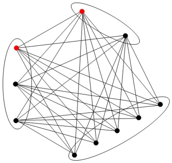
Example 2.

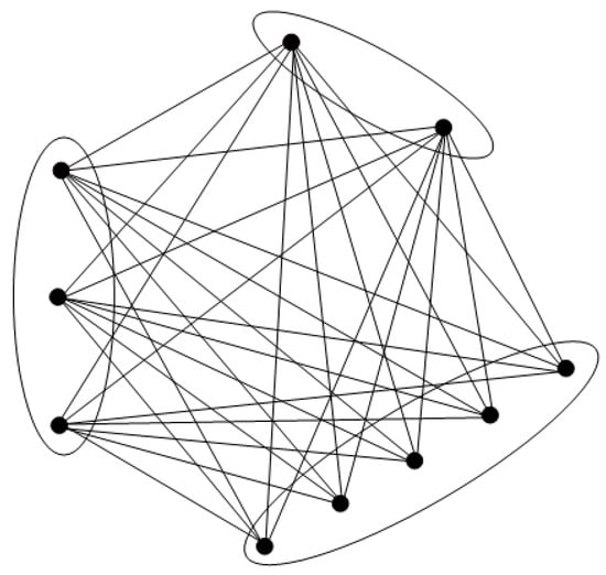
Let $K_{2,3,5}$ be the complete multipartite graph as given in Figure 4. Then, by Theorem 3, all of its vertices form a fault-tolerant metric generator and we obtain that $\beta \left(K_{2,3,5}\right)=10$.

Figure 4. The complete multipartite graph $K_{2,3,5}$ with the fault-tolerant metric generator (all vertices).

The following remark provides additional importance of Theorem 3.

Remark 2.

Note that Proposition 3 provides a counter example to Theorem 7 [53]. This shows that the characterization in Theorem 7 [53] is incorrect.

Based on this remark, we raise the following open problem.

Problem 1.

Let Γ be a connected graph on n vertices such that:

$${\beta }^{\prime }\left(\mathsf{\Gamma }\right)=n.$$

(5)

Are the complete graphs and the complete multipartite graphs the only graphs for which (5) holds? If yes, then characterize this extremal case, and if no, then provide additional examples satisfying (5).

3.3. Edge Metric Dimension

In this subsection, we determine the exact value of the edge metric dimension of the complete multipartite graphs.

Theorem 4.

Let $K_{t_1,t_2,\dots ,t_r}$ be the complete r-partite graph with $1\le t_1\le t_2\le \dots \le t_r$ and ${\displaystyle \sum _{i=1}^r}{t}_i=n$. Then:

$${\beta }_e\left(K_{t_1,t_2,\dots ,t_r}\right)=\sum _{i=1}^r{t}_i-r=n-r.$$

Proof. 

Let $T_i$ ($1\le i\le r$) be the $i^{\mathrm{th}}$ partite set with $|T_i|=t_i$. First, we show that ${\beta }_e\left(K_{t_1,t_2,\dots ,t_r}\right)\ge {\displaystyle \sum _{i=1}^r}{t}_i-r$. In order to show that, first, we need to prove that there exists an edge resolving set of cardinality ${\displaystyle \sum _{i=1}^r}{t}_i-r$ in $K_{t_1,t_2,\dots ,t_r}$. Let $x_i\in T_i$ be an arbitrary vertex in $T_i$, where $2\le i\le r$. Assume $S=V\left(K_{t_1,t_2,\dots ,t_r}\right)\setminus \{x_1,x_2,\dots ,x_r\}$ such that $\mid S\mid ={\displaystyle \sum _{i=1}^r}{t}_i-r$. We show that S is an edge resolving set in $K_{t_1,t_2,\dots ,t_r}$. Note that we have $V\left(K_{t_1,t_2,\dots ,t_r}\right)\setminus S=\{x_1,x_2,\dots ,x_r\}$.

Next, we assume that one of the partite sets contains at least two elements of $x_i(1\le i\le r)$. Without loss of generality, we assume Y to be that set and $x_1,x_2\in Y$. Let A be another partite set different from Y. For any $x\in A$ such that $x\in S$, consider the edges $e=x{x}_1$ and $f=x{x}_2$. Note that both e and f have distances 0 from x and one from any other element in S. Thus, both e and f have the same edge distance representations and this causes a contradiction to the fact that S is an edge resolving set. We may proceed with other partite sets in a similar way and it follows that any edge resolving set must contain all but (maybe) one element of every partite set. Since there exactly r number of partite sets, we obtain that ${\beta }_e\left(K_{t_1,t_2,\dots ,t_r}\right)\ge {\displaystyle \sum _{i=1}^r}{t}_i-r$.

On the contrary, let $x_i\in T_i$ where $1\le i\le r$ and let $S=V\left(K_{t_1,t_2,\dots ,t_r}\right)\setminus \{x_1,x_2,\dots ,x_r\}$. It can easily be checked that S is an edge resolving set as any two edges in $K_{t_1,t_2,\dots ,t_r}$ have different edge distance representations. Therefore, we obtain that ${\beta }_e\left(K_{t_1,t_2,\dots ,t_r}\right)\le {\displaystyle \sum _{i=1}^r}{t}_i-r$. The two inequalities complete the proof. □

The following example explains an application of Theorem 4.

Example 3.

Let $K_{2,3,5}$ be the complete multipartite graph as given in Figure 3. Then, its seven black vertices form an edge metric generator, i.e., a minimum edge resolving set of $K_{2,3,5}$. By Theorem 2, we obtain that ${\beta }_e\left(K_{2,3,5}\right)=10-3=7$.

The following remark gives additional importance of Theorem 4.

Remark 3.

It is worthy to mention that Theorem 4 generalizes Kelenc et al. (Remark 2 [22]) from the complete bipartite graphs to the complete multipartite graphs.

3.4. Mixed Metric Dimension

This section provides a formula for the mmd of complete multipartite graphs. It generalizes a result of Kelenc et al. [23], who computed the mmd of the complete bipartite case.

The following result calculates the mmd of the complete r-partite graph.

Theorem 5.

Let $K_{t_1,t_2,\dots ,t_r}$ be the complete r-partite graph with $1\le t_1\le t_2\le \dots \le t_r$ and ${\displaystyle \sum _{i=1}^r}{t}_i=n$. Then:

$${\beta }_m\left(K_{t_1,t_2,\dots ,t_r}\right)=\left\{\begin{array}{cc}{\displaystyle \sum _{i=1}^r}{t}_i-1,\hfill & \mathrm{if}{t}_i=2\mathrm{for}\mathrm{some}i;\hfill \\ {\displaystyle \sum _{i=1}^r}{t}_i-r,\hfill & \mathrm{Otherwise}.\hfill \end{array}\right.$$

Proof. 

By Theorems 2 and 4 and Equation (1), We obtain that ${\beta }_m\left(K_{t_1,t_2,\dots ,t_r}\right)\ge {\displaystyle \sum _{i=1}^r}{t}_i-r$. Let $T_i$ ($1\le i\le r$) be the $i^{\mathrm{th}}$ partite set with $|T_i|=t_i$. First, we assume that $t_1=2$. Suppose ${\beta }_e\left(K_{2=t_1,t_2,\dots ,t_r}\right)={\displaystyle \sum _{i=1}^r}{t}_i-1$ and assume L is the mixed resolving set of the smallest cardinality of $K_{2,t_2,\dots ,t_r}$. Notice that any edge resolving or simply resolving sets have to comprise $t_i-1$ elements of $T_i$, where $1\le i\le r$. We deduce that $\mid T_1\cap L\mid =1$ and $|T_i\cap L|=t_i-1$ for $i\in \{2,3,\dots ,r\}$. Let $y\in T_1\cap L$ and $z\in T_i\cap L$ for $i\in \{2,3,\dots ,r\}$. Then, $d(y,y)=0$ and $d(y,z)=1$. In addition, since $g=yz\in E_{K_{t_1,t_2,\dots ,t_r}}$, we have the vertex-edge distance $d(g,y)=0$ and $d(g,z)=0$. This shows that both y and g are not distinguished by L, which then leads to a contradiction to the minimality of L. A similar argument holds if any of the $t_i=2$ for $2\le i\le r$. This shows first part of the result by using Theorem 1.

Next, we assume that $t_i\ge 3$ for $1\le i\le r$. Assume L to be a minimum set comprising the ${\displaystyle \sum _{i=1}^r}{t}_i-r$ element in a way it considers all elements of $K_{t_1,t_2,\dots ,t_r}$ except one from every partite set. Note that L must distinguish all vertices/edges pairs of $K_{t_1,t_2,\dots ,t_r}$, since, by assumption, L is a minimum resolving and edge-resolving set. However, as $d(g,y)=\{0,1\}$ for any $g\in E_{K_{t_1,t_2,\dots ,t_r}}$ and $y\in K_{t_1,t_2,\dots ,t_r}$, and there exists at least one element in L which is at distance 2 from other vertices of $K_{t_1,t_2,\dots ,t_r}$ since $t_i\ge 3$ for $1\le i\le r$, it is convenient to see that L distinguishes all vertex-edge pair of $K_{t_1,t_2,\dots ,t_r}$. This implies the minimality of L with cardinality ${\displaystyle \sum _{i=1}^r}{t}_i-r$ and this completes the result. □

The following example illustrates an application of Theorem 5.

Example 4.

Let $K_{3,3,5}$ be the complete multipartite graph as depicted in Figure 5. Then, its eight black vertices form a mixed metric generator. By Theorem 5, we obtain that $\beta \left(K_{3,3,5}\right)=11-3=8$.

Figure 5. The complete multipartite graph $K_{3,3,5}$ with a mixed metric generator (black vertices).

It is important to remark the following:

Remark 4.

It is worth noting that Theorem 5 generalizes Proposition 4.2 [23] by Kelenc et al. [23].

4. Domination-Related Parameters

This section computes certain domination-related parameters, such as the domination number and the locating-dominating number of complete multipartite graphs.

4.1. Domination Number

The main purpose of this subsection is to calculate the domination number of complete multipartite graphs. The following theorem provides the exact value of the domination number.

Theorem 6.

Let $K_{t_1,t_2,\dots ,t_r}$ be the complete r-partite graph with $1\le t_1\le t_2\le \dots \le t_r$ and ${\displaystyle \sum _{i=1}^r}{t}_i=n$. Then

$$\gamma \left(K_{t_1,t_2,\dots ,t_r}\right)=\left\{\begin{array}{cc}1,\hfill & \mathrm{if}{t}_1=1;\hfill \\ 2,\hfill & \mathrm{Otherwise}.\hfill \end{array}\right.$$

Proof. 

Let $T_i$ be the $i^{\mathrm{th}}$ partite set having size $t_i$, i.e., $|T_i|:=t_i$.

Case 1: Assume that $t_1=1$.

This implies that $T_1$ has only one vertex, say, x. Then, $D=\left\{x\right\}$ is a dominating set, as x is adjacent to all the vertices in $T_i$ ($2\le i\le r$) i.e., $|D\bigcap N(x\left)\right|\ge 1$. This implies that $\gamma \left(K_{1,t_2,\dots ,t_r}\right)\le 1$. By definition, for any connected graph $\mathsf{\Gamma }$, $\gamma \left(\mathsf{\Gamma }\right)\ge 1$. This shows that $\gamma \left(K_{1,t_2,\dots ,t_r}\right)=1$.

Case 2: Assume that $2\le t_1\le t_2\le \dots \le t_r$.

This implies that every partite set has at least two vertices. Choose a vertex x from any partite set. Without loss of generality, we may take $x\in T_1$, such that $D=\left\{x\right\}$. Since $|T_1|\ge 2$, it contains at least one other vertex, say $y\in T_1$. Then $|D\bigcap N(y\left)\right|=0$ as $y\nsim x$ in $T_1$. This implies that D is not a dominating set of $K_{t_1,t_2,\dots ,t_r}$. Since $T_1$ was an arbitrary choice, we obtain that $\gamma \left(K_{t_1,t_2,\dots ,t_r}\right)\ge 2$.

On the other hand, let us take two elements from different partite sets in $K_{t_1,t_2,\dots ,t_r}$ in D. Without loss of generality, we assume that $D=\{x,y\}$ where $x\in T_1$ and $y\in T_2$. Then, all the vertices in $T_i$ ($3\le i\le r$) are adjacent to both x and y, i.e., $|D\bigcap N(u\left)\right|\ge 1$ for any $u\in T_i$ ($3\le i\le r$). Moreover, open neighborhoods of vertices other then x and y in $T_1$ and $T_2$, respectively, also have common elements with D which are either x or y. This implies that $|D\bigcap N(x^{\prime }\left)\right|=1$ for arbitrary $x^{\prime }\in T_1$ such that $x\ne x^{\prime }$ and $|D\bigcap N(y^{\prime }\left)\right|=1$ for any $y^{\prime }\in T_2$ such that $y\ne y^{\prime }$. This shows that D is a dominating set of $K_{t_1,t_2,\dots ,t_r}$ and $\gamma \left(K_{t_1,t_2,\dots ,t_r}\right)\le 2$. Combining it with other inequality, we obtain $\gamma \left(K_{t_1,t_2,\dots ,t_r}\right)=2$. This completes the proof. □

The following example illustrates an application of Theorem 6.

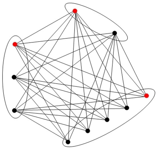
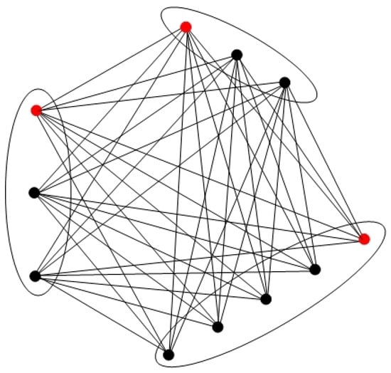
Example 5.

Let $K_{2,3,5}$ be the complete multipartite graph as depicted in Figure 6. Then, its two red vertices form a minimum dominating set. By Theorem 6, we obtain that $\gamma \left(K_{3,3,5}\right)=2$.

Figure 6. The complete multipartite graph $K_{2,3,5}$ with a minimum dominating set (red vertices).

The next subsection studies the locating-dominating number of graphs.

4.2. Locating-Dominating Number

First, we give the following characterization.

Theorem 7.

Let Γ be an n-vertex connected graph with $n\ge 2$. Then, $\mathsf{\Gamma }=K_n$ if and only if ${\gamma }_{l-d}\left(\mathsf{\Gamma }\right)=n-1$.

Proof. 

First, we assume that ${\gamma }_{l-d}\left(\mathsf{\Gamma }\right)=n-1$ and show that $\mathsf{\Gamma }$ is a complete graph. Since ${\gamma }_{l-d}\left(\mathsf{\Gamma }\right)=n-1$, it implies that there exists a locating-dominating set of cardinality $n-1$. Let $V\left(\mathsf{\Gamma }\right)=\{x_1,x_2,\dots ,x_n\}$. Without loss of generality, we may assume that $S=\{x_1,x_2,\dots ,x_{n-1}\}$. Then, we have that $x_n\in V\setminus S$.

We will show that $S\bigcap N\left[x_n\right]=S$. On the contrary, we suppose that $S\bigcap N\left[x_n\right]\ne S$. This implies that $N\left[x_n\right]\ne S$ such that $\left|N\right[x_n\left]\right|<n-1$. Then, it implies that there exists an $x^{\prime }\in V\left(\mathsf{\Gamma }\right)$ such that $x^{\prime }\ne x_n$ and $x^{\prime }\nsim x_n$. In that case, $S\setminus \left\{x\right\}$, where $x\in \{x_i:1\le i\le n-1\}$ is a locating-dominating set of $\mathsf{\Gamma }$, as we have $S\bigcap N\left[x_n\right]\ne S\bigcap N\left[x\right]$, since $S\bigcap N\left[x_n\right]=S\setminus \left\{x\right\}$ and $S\bigcap N\left[x\right]=S$. This contradicts the minimality of S. Therefore, $S\bigcap N\left[x_n\right]=S$, which implies that $x_n$ is adjacent to all the $x_i$, where $1\le i\le n-1$. Since $x_n$ was an arbitrary choice, we obtain that $\mathsf{\Gamma }=K_n$.

For necessity, we assume that $\mathsf{\Gamma }=K_n$. Then, any subset of $V\left(K_n\right)$ on $n-1$ vertices is a locating-dominating set of $K_n$. This gives ${\gamma }_{l-d}\left(K_n\right)\le n-1$. On the other hand, note that any subset of $V\left(K_n\right)$ on $n-2$ elements can never be a binary locating-dominating set, as the two elements in $S\setminus V\left(K_n\right)$ would have the same intersections. This implies that ${\gamma }_{l-d}\left(K_n\right)\ge n-1$. This shows that ${\gamma }_{l-d}\left(K_n\right)=n-1$, which completes the proof. □

The next proposition computes the exact value of the locating-dominating number of the complete bipartite graphs.

Proposition 1.

Let $K_{a,b}$ be the complete bipartite graph, where $1\le a\le b$. Then ${\gamma }_{l-d}\left(K_{a,b}\right)=a+b-2$.

Proof. 

Let $(A,B)$ be the bipartition of the vertex set of $K_{a,b}$ such that $\left|A\right|=a$ and $\left|B\right|=b$. Note that the induced subgraphs on A and B are the empty graphs $\overline{K_a}$ and $\overline{K_b}$, respectively. Let $x\in A$ and $y\in B$ be the arbitrary vertices in A and B, respectively. Note that the set $S=A\setminus \left\{x\right\}\bigcup B\setminus \left\{y\right\}$ is a binary locating-dominating set of $K_{a,b}$ as for both vertices x and y, the sets $S\cap N\left[x\right]=B\setminus \left\{y\right\}$ and $S\cap N\left[y\right]=A\setminus \left\{x\right\}$ are mutually disjoint. Since $\left|S\right|=a+b-2$, we obtain that ${\gamma }_{l-d}\left(K_{a,b}\right)\le a+b-2$.

Next, we prove the lower bound ${\gamma }_{l-d}\left(K_{a,b}\right)\ge a+b-2$. We will prove this by showing that ${\gamma }_{l-d}\left(K_{a,b}\right)$ cannot be $a+b-3$. On contrary, we suppose that ${\gamma }_{l-d}\left(K_{a,b}\right)=a+b-3$. This implies that there exists a locating-dominating set S of cardinality $a+b-3$. Let $x,y$, and z be the three vertices in $V\setminus S$. We distinguish the following possible cases for the vertices $x,y$ and z:

Case 1: All the three vertices, $x,y$, and z, belong to one partite set.

Without loss of generality, we may assume that $x,y$, and z, belong to A. Note that $S\cap N\left[x\right]=S\cap N\left[y\right]=S\cap N\left[z\right]=B$, which causes a contradiction to the fact any two such intersections must be disjointed. This suggests the following case:

Case 2: Either x, y, or z belongs to a partite set different from the other two vertices.

Without loss of generality, we may assume that $x\in A$ and $y,z\in B$. Then, $S\cap N\left[y\right]=S\cap N\left[z\right]=A$, which again causes a contradiction that S preserves to be a locating-dominating set.

Altogether, we obtain that S must contain exactly $a+b-2$ vertices, which completes the proof. □

The next proposition computes the exact value of the locating-dominating number of the complete tripartite graphs.

Proposition 2.

Let $K_{a,b,c}$ be the complete tripartite graph with $1\le a\le b\le c$. Then, ${\gamma }_{l-d}\left(K_{a,b,c}\right)=a+b+c-3$.

Proof. 

Let $(A,B,C)$ be the tripartition of $V\left(K_{a,b,c}\right)$, such that $\left|A\right|=a,\left|B\right|=b$ and $\left|C\right|=c$. For arbitrary vertices $x\in A$, $y\in B$ and $z\in C$, let $S=A\setminus \left\{x\right\}\bigcup B\setminus \left\{y\right\}\bigcup C\setminus \left\{z\right\}$. Note that S is a locating-dominating set of $K_{a,b,c}$, since $S\bigcap N\left[x\right]=B\setminus \left\{y\right\}\bigcup C\setminus \left\{z\right\}$, $S\bigcap N\left[y\right]=A\setminus \left\{x\right\}\bigcup C\setminus \left\{z\right\}$ and $S\bigcap N\left[z\right]=A\setminus \left\{x\right\}\bigcup B\setminus \left\{y\right\}$ are non-empty and mutually disjoint. Thus, we obtain that ${\gamma }_{l-d}\left(K_{a,b,c}\right)\le \left|S\right|=a+b+c-3$.

In order to complete the proof, we need to show that ${\gamma }_{l-d}\left(K_{a,b,c}\right)\ge a+b+c-3$. We show it by proving that ${\gamma }_{l-d}\left(K_{a,b,c}\right)>a+b+c-4$. On contrary, we assume that ${\gamma }_{l-d}\left(K_{a,b,c}\right)=a+b+c-4$. Thus, there exists a locating-dominating set of cardinality four and let S be that set. Let $V\left(K_{a,b,c}\right)\setminus S=\{w,x,y,z\}$. We distinguish the following possible cases for the vertices $w,x,y$, and z as follows:

Case 1: All $w,x,y$, and z belong to one partite set.

Without loss of generality, we may assume that $\{w,x,y,z\}\subset A$. Assuming it would generate $S\bigcap N\left[w\right]=S\bigcap N\left[x\right]=S\bigcap N\left[y\right]=S\bigcap N\left[z\right]=B\bigcup C$, which causes a contradiction to the fact that S is a locating-dominating set of $K_{a,b,c}$.

Case 2: All $w,x,y$, and z belong to exactly two partite sets.

Subcase 2.1: One partite set is singleton.

Without loss of generality, we may assume that $\{w,x,y\}\subset A$ and $z\in B$. Then, the same intersections $S\bigcap N\left[w\right]=S\bigcap N\left[x\right]=S\bigcap N\left[y\right]=C\bigcup B\setminus \left\{z\right\}$ cause a contradiction that S is a binary-locating dominating set.

Subcase 2.2: Both partite sets have cardinality 2.

Similar to the previous cases, without loss of generality, we may assume that $\{w,x\}\subset A$ and $\{y,z\}\subset B$. In this case, we obtain that $S\bigcap N\left[w\right]=S\bigcap N\left[x\right]=C\bigcup B\setminus \{y,z\}$ and $S\bigcap N\left[y\right]=S\bigcap N\left[z\right]=C\bigcup A\setminus \{w,x\}$, which is a contradiction again.

Case 3: All $w,x,y$, and z belong to exactly three partite sets.

Without loss of generality, we may assume that $w\in A$, $x\in B$, and $\{y,z\}\in C$. Assuming this would generate $S\bigcap N\left[z\right]=A\setminus \left\{w\right\}\bigcup B\setminus \left\{x\right\}=S\bigcap N\left[y\right]$. Thus, the two intersections are not mutually disjoint which causes a contradiction.

Combining all the possible case, we find that S is not a locating-dominating set of $K_{a,b,c}$. Since S was an arbitrary set of cardinality four, we obtain that ${\gamma }_{l-d}\left(K_{a,b,c}\right)>a+b+c-4\ge a+b+c-3$. This completes the proof. □

Next, we show the main result of this subsection.

Theorem 8.

Let $K_{t_1,t_2,\dots ,t_r}$ be the complete r-partite graph with $1\le t_1\le t_2\le \dots \le t_r$ and ${\displaystyle \sum _{i=1}^r}{t}_i=n$. Then:

$${\gamma }_{l-d}\left(K_{t_1,t_2,\dots ,t_r}\right)=\sum _{i=1}^r{t}_i-r.$$

(6)

Proof. 

We prove the result by applying induction on r, which is the number of partite sets in $K_{t_1,t_2,\dots ,t_r}$. By Propositions 1 and 2, the result is true for $r=2$ and $r=3$, respectively. Now, let the assertion be valid for $r=k$ as an induction step. We show that the result is true for $r=k+1$ to complete the proof.

Let $T_i$ ($1\le i\le r$) be the $i^{\mathrm{th}}$ partite set of $K_{t_1,t_2,\dots ,t_r}$, where $|T_i|:=t_i$. Since (8) holds for $r=k$, we obtain that:

$${\gamma }_{l-d}\left(K_{t_1,t_2,\dots ,t_k}\right)=\sum _{i=1}^k{t}_i-k.$$

(7)

This implies that there exists a minimum locating-dominating set of cardinality ${\displaystyle \sum _{i=1}^k}{t}_i-k$ in $K_{t_1,t_2,\dots ,t_k}$. Let S be the minimum locating-dominating set of cardinality ${\displaystyle \sum _{i=1}^k}{t}_i-k$. in $K_{t_1,t_2,\dots ,t_k}$. Let $U=\{x_i\in T_i:1\le i\le k\}$ and $S=V\left(K_{t_1,t_2,\dots ,t_k}\right)\setminus U$, then S comprises $t_i-1$ elements from every $T_i$ where $1\le i\le r$. Note that S is a locating-dominating set of $K_{t_1,t_2,\dots ,t_k}$, since $S\bigcap N\left[x_i\right]\ne S\bigcap N\left[x_j\right]$ for $1\le i<j\le k$ and $S\bigcap N\left[x_i\right]=S\setminus T_i$ $1\le i\le k$. Moreover, S is minimum as the inclusion of more than one vertices from any partite set $T_i$ in S would cause a contradiction, as the two vertices from the same partite set would have the same intersections. Moreover, the minimality of S follows from (7), as S is a locating-dominating set.

Now, we add ($k+1$)${}^{\mathrm{th}}$ partite set, say $T_{k+1}$, to $K_{t_1,t_2,\dots ,t_k}$ to obtain $K_{t_1,t_2,\dots ,t_k,t_{k+1}}$. For any $x^{\prime }\in T_{k+1}$, let $S^{\prime }=S\bigcup \left\{x^{\prime }\right\}$. Note that $S^{\prime }$ is a locating-dominating set of $K_{t_1,t_2,\dots ,t_{k+1}}$ since $S^{\prime }\bigcap N\left[x^{\prime }\right]\ne S^{\prime }\bigcap N\left[x_i\right]$ for $1\le i\le k$ and $S^{\prime }\bigcap N\left[x^{\prime }\right]=S^{\prime }\setminus T_{k+1}$. Moreover, $S^{\prime }$ is minimum as S is minimum in $K_{t_1,t_2,\dots ,t_k}$. Since $\left|S\right|={\displaystyle \sum _{i=1}^{k+1}}{t}_i-(k+1)$, we obtain that:

$${\gamma }_{l-d}\left(K_{t_1,t_2,\dots ,t_{k+1}}\right)=\sum _{i=1}^{k+1}{t}_i-(k+1).$$

By applying the induction hypothesis on r, the proof is finished. □

The following example illustrates an application of Theorem 8.

Example 6.

Let $K_{2,3,5}$ be the complete multipartite graph as depicted in Figure 3. Then, its seven black vertices form a minimum locating-dominating set. By Theorem 8, we obtain that ${\gamma }_{l-d}\left(K_{2,3,5}\right)=10-3=7$.

The next section studies an interaction between resolvability and domination of graphs.

5. An Interaction between Resolvability and Domination

The main purpose of this section is to study the metric-locating-dominating number of complete multipartite graphs by using their locating-dominating and the resolvability structures.

Metric-Locating-Dominating Number

In this section, we compute the metric-locating-dominating number of complete multipartite graphs.

First, we show the following lemma.

Lemma 1.

Let Γ be a connected graph such that either $\beta \left(\mathsf{\Gamma }\right)=r=\gamma \left(\mathsf{\Gamma }\right)$ or $\beta \left(\mathsf{\Gamma }\right)=r={\gamma }_{l-d}\left(\mathsf{\Gamma }\right)$. Then, ${\gamma }_{mld}\left(\mathsf{\Gamma }\right)=r$.

Proof. 

We divide our discussion into the following two cases:

Case 1: Assume $\beta \left(\mathsf{\Gamma }\right)=r=\gamma \left(\mathsf{\Gamma }\right)$.

This implies that there exists a metric-locating-dominating set on r number of vertices, since both the metric dimension and domination number equal to r. Moreover, such a metric-locating-dominating number is minimum because there exists a minimum resolving set and a minimum dominating set, both having cardinality r. This implies that ${\gamma }_{mld}\left(\mathsf{\Gamma }\right)=r$.

Case 2: Assume $\beta \left(\mathsf{\Gamma }\right)=r={\gamma }_{l-d}\left(\mathsf{\Gamma }\right)$.

There exists a dominating set of cardinality r, since ${\gamma }_{l-d}\left(\mathsf{\Gamma }\right)=r$. Moreover, $\mathsf{\Gamma }$ has a minimum resolving set of cardinality r, since $\beta \left(\mathsf{\Gamma }\right)=r$. Thus, there exists a metric-locating-dominating set of cardinality r, say M. Note that M is minimum as the resolving set of cardinality r is minimum in $\mathsf{\Gamma }$. This shows that ${\gamma }_{mld}\left(\mathsf{\Gamma }\right)=r$, which completes the proof. □

By Lemma 1 and Theorems 8 and 2, we have the following corollary.

Theorem 9.

Let $K_{t_1,t_2,\dots ,t_r}$ be the complete r-partite graph with $1\le t_1\le t_2\le \dots \le t_r$ and ${\displaystyle \sum _{i=1}^r}{t}_i=n$. Then:

$${\gamma }_{mld}\left(K_{t_1,t_2,\dots ,t_r}\right)=\sum _{i=1}^r{t}_i-r.$$

The following example illustrates an application of Theorem 9.

Example 7.

Let $K_{2,3,5}$ be the complete multipartite graph as depicted in Figure 3. Then, its seven black vertices form a minimum metric locating-dominating set. By Theorem 9, we obtain that ${\gamma }_{mld}\left(K_{2,3,5}\right)=10-3=7$.

Theorem 9 computes the metric-locating-dominating number of complete multipartite graphs, which is the first result of its kind in the theory of metric-locating-dominating number of graphs.

6. Conclusions

This paper studied the metric, fault-tolerant metric, edge metric, mixed-metric dimensions, the domination number, locating-dominating number, and metric-locating-dominating number for complete multipartite graphs. These results generalize various results in the literature from complete bipartite to complete multipartite graphs. Especially, we showed that the fault-tolerant metric dimension of n-vertex complete multipartite graphs is n. This, in turn, provides an infinite family of counterexamples to Theorem 7 [53] by Raza et al., who showed that the complete graphs are the only graphs with fault-tolerant metric dimension n. Section 3.2 points out an error in the proof of Theorem 7 [53] by Raza et al.

In the future, the authors intend to study the following open problems on the fault-tolerant resolvability of graphs:

Problem 2. Study graphs whose mixed metric dimension is smaller than the metric dimension.

Problem 3. Are there graphs whose fault-tolerant metric dimension is smaller than or equal to their metric dimension?

References

- Slater, P.J. Leaves of trees. Congress. Numer. 1975, 14, 549–559. [Google Scholar]
- Harary, F.; Melter, R.A. On the metric dimension of a graph. Ars Combin. 1976, 2, 191–195. [Google Scholar]
- Buckley, F.; Harary, F. Distances in Graphs; Addison-Wesley Publishing Company: Boston, MA, USA, 1990. [Google Scholar]
- Chartrand, G.; Zhang, P. The theory and applications of resolvability in graphs: A survey. Congress. Numer. 2003, 160, 47–68. [Google Scholar]
- Khuller, S.; Raghavachari, B.; Rosenfeld, A. Landmarks in graphs. Discrete Appl. Math. 1996, 70, 217–229. [Google Scholar] [CrossRef]
- Chartrand, G.; Eroh, L.; Johnson, M.A.; Oellermann, O.R. Resolvability in graphs and metric dimension of a graph. Discrete Appl. Math. 2000, 105, 99–113. [Google Scholar] [CrossRef]
- Beerloiva, Z.; Eberhard, F.; Erlebach, T.; Hall, A.; Hoffmann, M.; Mihalák, M.; Ram, L.S. Network discovery and verification. IEEE J. Sel. Area Commun. 2006, 24, 2168–2181. [Google Scholar] [CrossRef]
- Raza, H.; Hayat, S.; Pan, X.-F. Binary locating-dominating sets in rotationally-symmetric convex polytopes. Symmetry 2018, 10, 727. [Google Scholar] [CrossRef]
- Liu, K.; Abu-Ghazaleh, N. Virtual coordinate backtracking for void traversal in geometric routing. Lect. Notes Comput. Sci. 2006, 4104, 46–59. [Google Scholar]
- Harary, F. Status and contrastatus. Sociometry 1959, 22, 23–43. [Google Scholar] [CrossRef]
- Abas, M.; Vetrik, T. Metric domination of directed Cayley graphs of metacyclic groups. Theor. Comput. Sci. 2020, 809, 61–72. [Google Scholar] [CrossRef]
- Bailey, R.F.; Cameron, P.J. Basie size, metric dimension and other invariants of groups and graphs. Bull. Lond. Math. Soc. 2011, 43, 209–242. [Google Scholar] [CrossRef]
- Bailey, R.F.; Meagher, K. On the metric dimension of Grassmann graphs. Discrete Math. Theor. Comput. Sci. 2011, 13, 97–104. [Google Scholar] [CrossRef]
- Buczkowski, P.S.; Chartrand, G.; Poisson, C.; Zhang, P. On k-dimensional graphs and their bases. Period. Math. Hung. 2003, 46, 9–15. [Google Scholar] [CrossRef]
- Cáceres, J.; Hernando, C.; Mora, M.; Pelayoe, I.M.; Puertas, M.L.; Seara, C.; Wood, D.R. On the metric dimension of cartesian products of graphs. SIAM J. Discrete Math. 2007, 21, 423–441. [Google Scholar] [CrossRef]
- Cáceres, J.; Hernando, C.; Mora, M.; Puertas, M.L.; Pelayo, I.M. On the metric dimension of infinite graphs. Electron. Notes Disc. Math. 2009, 35, 15–20. [Google Scholar] [CrossRef]
- Fehr, M.; Gosselin, S.; Oellermann, O. The metric dimension of Cayley digraphs. Discrete Math. 2006, 306, 31–41. [Google Scholar] [CrossRef]
- Imran, M.; Siddiqui, H.M.A. Computing the metric dimension of convex polytopes generated by wheel related graphs. Acta Math. Hung. 2016, 149, 10–30. [Google Scholar] [CrossRef]
- Saputro, S.W.; Simanjuntak, R.; Uttunggadewa, S.; Assiyatun, H.; Baskoro, E.T.; Salman, A.N.M.; Bača, M. The metric dimension of the lexicographic product of graphs. Discrete Math. 2013, 313, 1045–1051. [Google Scholar] [CrossRef]
- Siddiqui, H.M.A.; Imran, M. Computing the metric dimension of wheel related graphs. Appl. Math. Comput. 2014, 242, 624–632. [Google Scholar]
- Yero, I.G.; Kuziak, D.; Rodríguez-Velázquez, J.A. On the metric dimension of corona product graphs. Comput. Math. Appl. 2011, 61, 2793–2798. [Google Scholar] [CrossRef]
- Kelenc, A.; Tratnik, N.; Yero, I.G. Uniquely identifying the edges of a graph: The edge metric dimension. Discrete Appl. Math. 2018, 251, 204–220. [Google Scholar] [CrossRef]
- Kelenc, A.; Kuziak, D.; Taranenko, A.; Yero, I.G. Mixed metric dimension of graphs. Appl. Math. Comput. 2017, 314, 429–438. [Google Scholar]
- Filipovic, V.; Kartelj, A.; Kratica, J. Edge metric dimension of some generalized Petersen graphs. Results Math. 2019, 74, 1–15. [Google Scholar] [CrossRef]
- Knor, M.; Majstorovic, S.; Toshi, A.T.M.; Škrekovski, R.; Yero, I.G. Graphs with the edge metric dimension smaller than the metric dimension. Appl. Math. Comput. 2021, 401, 126076. [Google Scholar] [CrossRef]
- Zhang, Y.; Gao, S. On the edge metric dimension of convex polytopes and its related graphs. J. Comb. Optim. 2020, 39, 334–350. [Google Scholar] [CrossRef]
- Zhu, E.; Taranenko, A.; Shao, Z.; Xu, J. On graphs with the maximum edge metric dimension. Discrete Appl. Math. 2019, 257, 317–324. [Google Scholar] [CrossRef]
- Danas, M.M. The mixed metric dimension of flower snarks and wheels. Open Math. 2021, 19, 629–640. [Google Scholar] [CrossRef]
- Sedlar, J.; Škrekovski, R. Extremal mixed metric dimension with respect to the cyclomatic number. Appl. Math. Comput. 2021, 404, 126238. [Google Scholar] [CrossRef]
- Sedlar, J.; Škrekovski, R. Mixed metric dimension of graphs with edge disjoint cycles. Discrete Appl. Math. 2021, 300, 1–8. [Google Scholar] [CrossRef]
- Hernando, C.; Mora, M.; Slater, P.J.; Wood, D.R. Fault-tolerant metric dimension of graphs. In Joint Proceedings of the International Instructional Workshop on Convexity in Discrete Structures, Thiruvananthapuram, India, 2006 and the International Workshop on Metric and Convex Graph Theory, Barcelona, Spain, 2006; Lecture Notes Series No. 5; Ramanujan Mathematical Society: Mysore, India, 2008; pp. 81–85. [Google Scholar]
- Hayat, S.; Khan, A.; Malik, M.Y.H.; Imran, M.; Siddiqui, M.K. Fault-tolerant metric dimension of interconnection networks. IEEE Access 2020, 8, 145435–145445. [Google Scholar] [CrossRef]
- Raza, H.; Hayat, S.; Pan, X.-F. On the fault-tolerant metric dimension of certain interconnection networks. J. Appl. Math. Comput. 2019, 60, 517–535. [Google Scholar] [CrossRef]
- Raza, H.; Hayat, S.; Pan, X.-F. On the fault-tolerant metric dimension of convex polytopes. Appl. Math. Comput. 2018, 339, 172–185. [Google Scholar] [CrossRef]
- Siddiqui, H.M.A.; Hayat, S.; Khan, A.; Imran, M.; Razzaq, A.; Liu, J.-B. Resolvability and fault-tolerant resolvability structures of convex polytopes. Theor. Comput. Sci. 2014, 769, 114–128. [Google Scholar] [CrossRef]
- Haynes, T.W.; Hedetniemi, S.; Slater, P. Fundamentals of Domination in Graphs; CRC Press: New York, NY, USA, 1998. [Google Scholar]
- Haynes, T.W.; Henning, M.A.; Howard, J. Locating and total dominating sets in trees. Discrete Appl. Math. 2006, 154, 1293–1300. [Google Scholar] [CrossRef]
- Charon, I.; Hudry, O.; Lobstein, A. Extremal cardinalities for identifying and locating-dominating codes in graphs. Discrete Math. 2007, 307, 356–366. [Google Scholar] [CrossRef]
- Honkala, I.; Hudry, O.; Lobstein, A. On the ensemble of optimal dominating and locating-dominating codes in a graph. Inform. Process. Lett. 2015, 115, 699–702. [Google Scholar] [CrossRef]
- Honkala, I.; Laihonen, T. On locating-dominating sets in infinite grids. Eur. J. Combin. 2006, 27, 218–227. [Google Scholar] [CrossRef]
- Slater, P.J. Fault-tolerant locating-dominating sets. Discrete Math. 2002, 249, 179–189. [Google Scholar] [CrossRef]
- Seo, S.J.; Slater, P.J. Open neighborhood locating-dominating sets. Australas. J. Combin. 2010, 46, 109–119. [Google Scholar]
- Seo, S.J.; Slater, P.J. Open neighborhood locating-dominating in trees. Discrete Appl. Math. 2011, 159, 484–489. [Google Scholar] [CrossRef]
- Simić, A.; Bogdanović, M.; Milošević, J. The binary locating-dominating number of some convex polytopes. Ars Math. Contemp. 2017, 13, 367–377. [Google Scholar] [CrossRef]
- Hernando, C.; Mora, M.; Pelayo, I.M. LD-graphs and global location-domination in bipartite graphs. Electron. Notes Discrete Math. 2014, 46, 225–232. [Google Scholar] [CrossRef]
- Slater, P.J. Domination and location in acyclic graphs. Networks 1987, 17, 5–64. [Google Scholar] [CrossRef]
- Slater, P.J. Locating dominating sets and locating-dominating sets. In Graph Theory, Combinatorics, and Algorithms; Alavi, Y., Schwenk, A., Eds.; John Wiley & Sons: Hoboken, NJ, USA, 1995; Volume 2, pp. 1073–1079. [Google Scholar]
- Ebrahimi, B.J.; Jahanbakht, N.; Mahmoodian, E.S. Vertex domination of generalized Petersen graphs. Discrete Math. 2009, 309, 4355–4361. [Google Scholar] [CrossRef]
- Tong, C.; Lin, X.; Yang, Y.; Luo, M. 2-rainbow domination of generalized Petersen graphs P(n, 2). Discrete Appl. Math. 2009, 157, 1932–1937. [Google Scholar] [CrossRef]
- Xu, G. 2-rainbow domination in generalized Petersen graphs P(n, 3). Discrete Appl. Math. 2009, 157, 2570–2573. [Google Scholar] [CrossRef]
- Xueliang, F.; Yuansheng, Y.; Baoqi, J. On the domination number of generalized Petersen graphs P(n, 2). Discrete Math. 2009, 309, 2445–2451. [Google Scholar]
- Yan, H.; Kang, L.; Xu, G. The exact domination number of the generalized Petersen graphs. Discrete Math. 2009, 309, 2596–2607. [Google Scholar] [CrossRef][Green Version]
- Raza, H.; Hayat, S.; Imran, M.; Pan, X.-F. Fault-tolerant resolvability and extremal structures of graphs. Mathematics 2019, 7, 78. [Google Scholar] [CrossRef]
- Diudea, M.V.; Gutman, I.; Jäntschi, L. Molecular Topology; Nova Science Publishers: New York, NY, USA, 2001. [Google Scholar]
- Joiţa, D.-M.; Jäntschi, L. Extending the characteristic polynomial for characterization of C20 fullerene congeners. Mathematics 2017, 5, 84. [Google Scholar] [CrossRef]
- Jäntschi, L. The eigenproblem translated for alignment of molecules. Symmetry 2019, 11, 1027. [Google Scholar] [CrossRef]
- Jäntschi, L. Structure-property relationships for solubility of monosaccharides. Appl. Water Sci. 2019, 9, 38–49. [Google Scholar] [CrossRef]
- Saputro, S.W.; Baskoro, E.T.; Salman, A.N.M.; Suprijanto, D. The metric dimension of a complete n-partite graph and its Cartesian product with a path. J. Comb. Math. Comb. Comput. 2009, 71, 283–293. [Google Scholar]
Publisher’s Note: MDPI stays neutral with regard to jurisdictional claims in published maps and institutional affiliations. |
© 2022 by the authors. Licensee MDPI, Basel, Switzerland. This article is an open access article distributed under the terms and conditions of the Creative Commons Attribution (CC BY) license (https://creativecommons.org/licenses/by/4.0/).