1. Introduction
The construction and operation of buried pipelines in remote permafrost areas leads to thawing and thereby reducing the subgrade capacity of frozen soil. Minor soil temperature fluctuations in the range of 2–5 °C contribute to significant changes in spatial positioning and may cause damage to objects. A geotechnical system monitors the temperature regime of the soil to identify hazardous processes in permafrost at the operational stage. At the local level of this system, there are strings of sensors (thermistors) loaded at various depths in specially equipped thermowells for the simultaneous measurement of temperature at multiple points. Measurements, converted to digital format, are transmitted to the reading, storage, and display devices (controllers). Controllers periodically poll the sensors in the string and read the numbers for the connection lines to sort the measurements by the depth and save them on local storage devices. Fiber or wireless networks are used at the regional level for accessing local archives [
1]. The global level of a geotechnical monitoring system for an extended pipeline includes web servers for synchronization, integration, processing, and maintenance of measures and saving prepared information in a specialized global data warehouse. A longer operating time increases the number of exogenous processes, makes it necessary to install additional thermowells, and accumulates a large quantity of information that is difficult to analyze with classical statistical methods. For completing data processing steps, unified scripts and schemes are created to integrate them into a reproducible workflow.
The purpose of this study is to offer an express, visual, reasonably accurate approach to locate and predict heat losses of the buried oil pipeline. An approach that would be available to oil operators without expert knowledge.
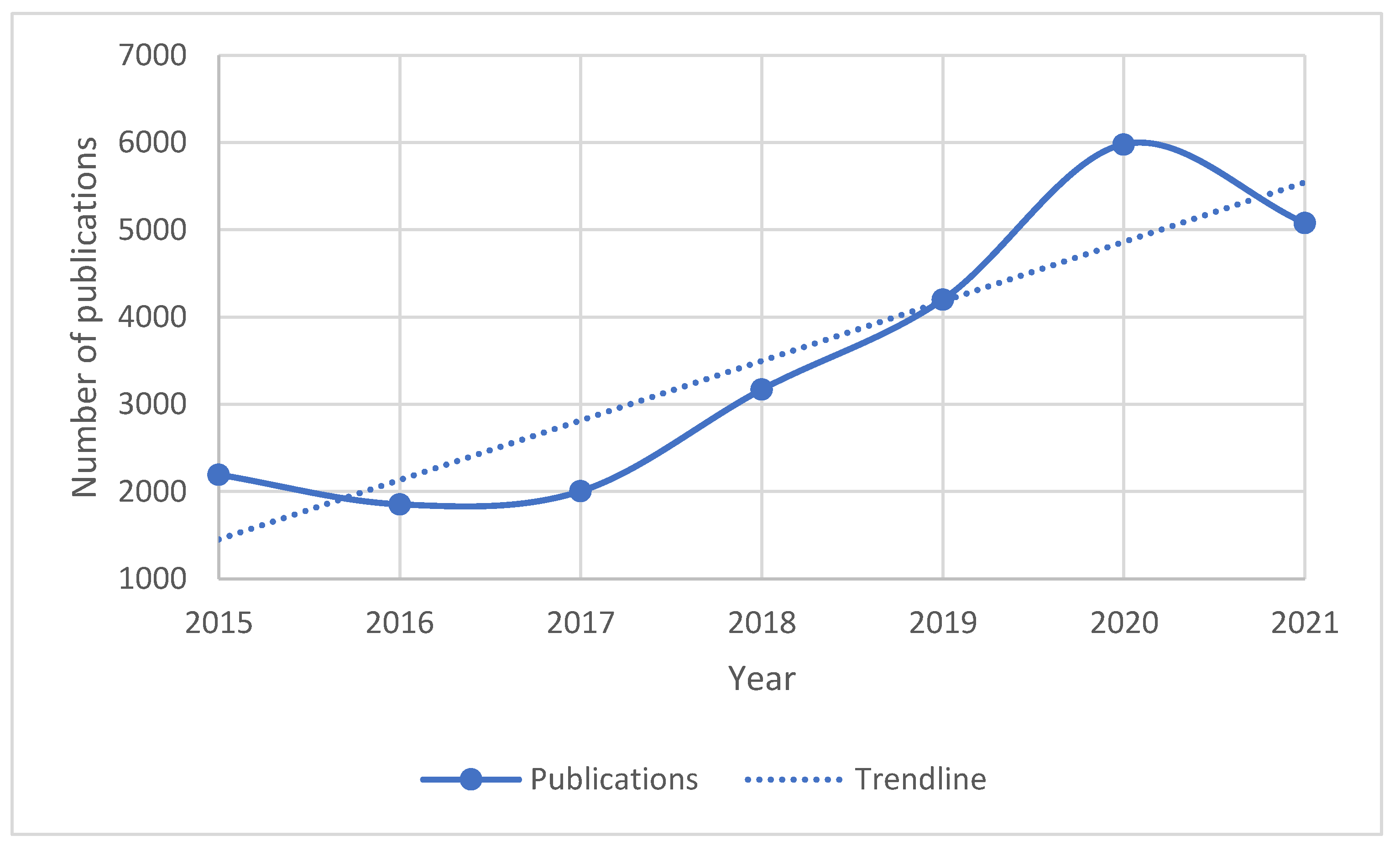
According to the Dimensions platform (
www.dimensions.ai, last accessed on 20 May 2022) that provides access to grants, publications, patents, and other sources, the number of publications in which remote geotechnical monitoring was mentioned in the years 2015–2021 is on the rise (
Figure 1).
Analysis of publications on the topic of the study went in three main directions: organization of a remote geotechnical network, preprocessing of geotechnical data, and comparison of forecasting models that consider the seasonality and non-stationarity of the time series. The first group of articles discusses the causes of data transfer errors. The authors of [
2] created a cloud system to remotely monitor the moisture of fertile soil. They note that under conditions of unstable network connection in the rural area, the collected data contain a significant number of omissions. The quality of an open atmospheric optical channel is reported [
3] to be affected by the frequency of weather changes, the fluctuations of the supports, and the scintillation. Additionally, it is demonstrated that long distances and electromagnetic interference distort the signal, and the thermistors readings are affected by moisture intrusion [
4]. Therefore, sensor data must be carefully prepared for prediction.
The second group presents publications offering preprocessing schemes of raw data for the subsequent identification or prediction of the state of the system under study. Data processing pipelines (dimensional modification, indexing, aggregation, time-series oversampling, etc.) are derived from the book by the author of a Python library [
5]. The regional-scale hydrological system model is a good example of applying a data preprocessing pipeline to heterogeneous datasets [
6]. Each type of climate data (e.g., temperature, wind speed) is tied to a uniform grid with a predetermined pitch, and investigators note that most of the time is spent preparing and binding data rather than forecasting from ready-made models. Further investigation [
7] defines aggregation as the main preprocessing procedure for sensor data due to its volume and monotony. Based on this, the authors conclude that the significance of sensor data is mainly in discovering trends.
Below is a third group of articles where the forecasting method is used, highlighting the trend in the data. Traditionally, a time series containing seasonality is thought of as a mixture of trend-cyclical, seasonal, and irregular components, assuming that these components are independent and additive or multiplicative. Having a decade and half period of observation, various trends in fumarole temperatures are detected when applying a thermal model, considering three temperature subcycles: the annual cycle, representing the daily-averaged temperature; the daily cycle, representing the instantaneous temperature; and the weather-change cycle, which is divided into two parts to represent both the daily-averaged and the instantaneous temperature [
8]. Monitoring is limited to only a few sites, but the observed trends help define the most critical fumaroles in the area.
To use the powerful model named ARIMA (autoregressive integrated moving average), researchers must check whether the series contains trends, seasonality, emissions, nonconstant variances, and other non-stationarities. The more non-stationarity manifests itself, the stronger the transformation that must be used [
9]. The weak point of the model is that the researcher is forced to control the transformation effect visually. As a result, the model is challenging to use for engineers who are not professionally trained experts [
10]. Neural network-based prediction methods (e.g., LSTM, ANN) require more data, even for short-term prediction [
11]. Therefore, the data referenced in the ANN simulation are the hourly activity schedules of more than 5000 data sources, containing 6 features and collected for a year, and yet the authors need to simulate additional data to train the model [
12].
In addition to those listed, there are numerical algorithms for solving thermal conductivity problems based on the finite volume method [
13] and the finite difference method [
14]. Their fundamental disadvantage is the use of small-scale grid spacing, which leads to high overhead costs for extended pipelines [
15]. Similarly, fast Fourier transformation focusing on trend and harmonics is used to separate seasonal temperature variations from the influence of the oil pipeline [
16]. The main limitations of the fast Fourier transformation are the use of data arrays of lengths equal to the degree of two and noticeable distortion of the results at a low sample rate.
A recent study [
17] compares long short-term memory (LSTM) and a three-component model named Prophet for predicting air temperature. The study leverages massive historical data on daily maximum and minimum air temperatures for more than 5 years. The authors note that using time as a regressor, Prophet fits piecewise linear and nonlinear saturating growth functions to define the first component. The second component that defines seasonality effects is fitted by using a Fourier series, and the third component could be defined by an analyst providing a custom list of past and future events. The result showed that, for minimum temperature, Prophet performs better on maximum air temperature while LSTM performs better on minimum air temperature.
A growing number of articles and patents enlisted in [
18] on monitoring sites in permafrost areas over the last two decades has enabled a discussion regarding the topical significance of the issue. Soil temperatures at depths of 7–8 m are known to be significantly different from air temperatures, particularly in summer and autumn. Thawed soils with varying concentrations of ice produce various sediments. Therefore, the predicted change in soil temperature in three dimensions, taking into account the seasonal component, highlights the impact of the pipeline transporting heated oil. To achieve this aim, we represent soil temperatures as time series, define additional features that improve the accuracy of the forecasting model, select uncorrelated features to decrease the dimensionality of the model, learn the regression model of the soil temperature dynamics over time and estimate its quality.
2. Materials and Methods
Geotechnical monitoring systems tend to comprise groups of sensors in thermometric wells along the routes of the pipelines; the sensors are linked with wired or wireless technologies and measurements are obtained using web-based software. The geotechnical dataset was collected over a year at 13 locations along the pipeline. It represents daily measurements of soil temperature at depths of up to 15 m during daylight hours [
19].
Fourteen open-source Python libraries are applied to manipulate, visualize, and obtain geotechnical data. Primary analysis was made with a library named Numpy. It facilitates advanced mathematical operations on big data. The Pandas library provides flexible data structures to work with structured (tabular, multidimensional, potentially heterogeneous) and time-series data. The library, named Pandas-profiling, is a tool to preview, explore, and summarize the statistical information of a dataset. Python packages such that SciPy, Sklearn, and Statsmodels are used for data manipulation. All data visualizations were made with Matplotlib, Pandas.plotting, Prophet.plot, and Seaborn. We performed extended data analysis with a library named Association_metrics. It provides tools to measure the degree of nonlinear association among other features. The feature engineering for time series was based on the Calendar package. The Facebook Prophet and SciPy.Interpolate packages provide models for predicting time series. The programming code was created in the Google Research product, named Colaboratory, enabling developers to write and execute Python code via a browser.
2.1. Initial Data Structure
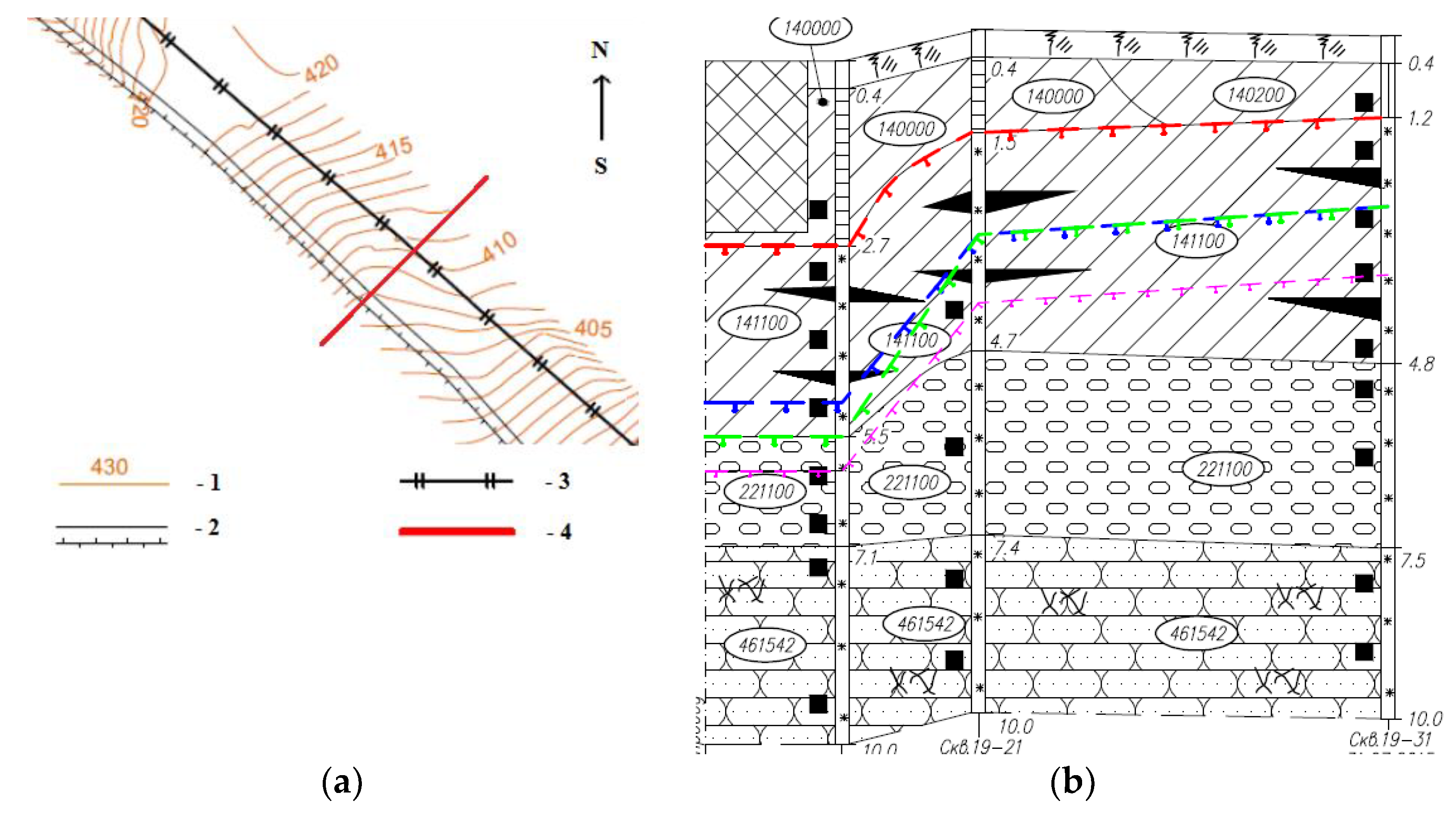
Within the geotechnical monitoring system, triples of thermowells are installed along the pipeline route, mainly in the areas where exogenous processes are developing (
Figure 2a). Each thermowell contains 8–12 thermistors installed at different depths of the soil (
Figure 2b).
The initial data, which were temperature measurements, could be represented as a 4D array, such that each dimension contained data about the following:
- -
location along the route as the numbers of thermometric wells in which the garlands of temperature sensors are installed;
- -
distance from the pipe, as there are three thermometric wells inline at every location at 2, 4, and 10 m, respectively;
- -
depth as the levels of soil’s depth at which each temperature sensor of a garland was installed from 0 to 15 m;
- -
time as the moments of temperature fixations.
The initial data measured 1.7+ megabytes and were distributed across 51 features.
2.2. Two-Step Approach of Forecasting Temperatures Based upon a Geotechnical Dataset
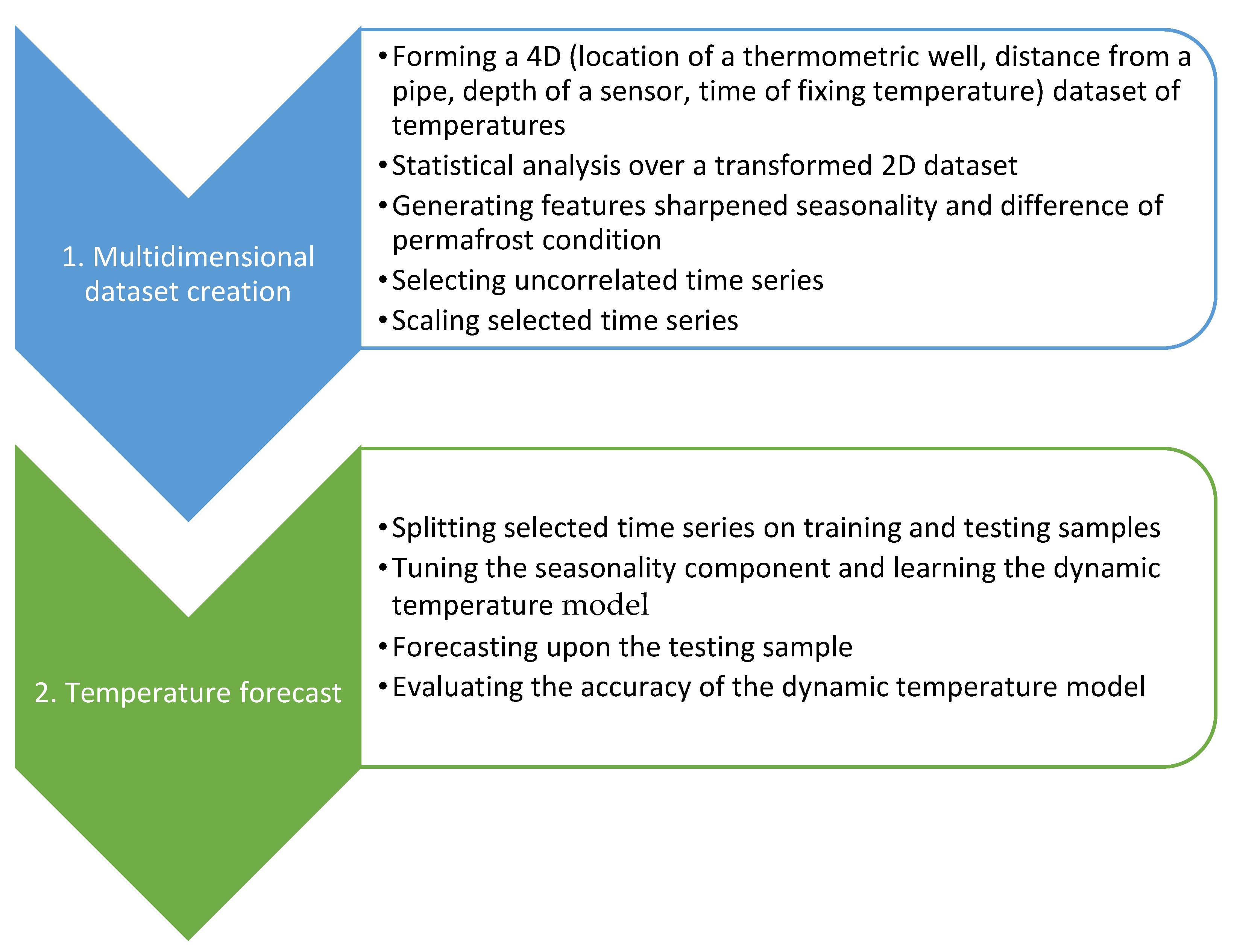
Figure 3 shows the two-step approach to analyze the dynamics of the soil temperatures along the route of an oil pipeline that crosses permafrost zones.
Our approach differs from the known approaches as we transform the collected 4D array to 2D without losing information; add new features, underlining seasonality, and permafrost condition; conduct both linear and nonlinear correlation analyses, selecting time series significant in the forecasting model; and finally, we train the Prophet model using data form the thermowell triples.
2.3. Statistical Analysis on a Transformed Dataset
In the original dataset (
Table 1), the daily temperature measurements collected by the geotechnical system were naturally grouped around the date of measurement and the number of the thermowells’ triples (groups of three thermowells). This data view contained four dimensions for every temperature measurement: location, distance from the pipe, depth, and time. This view is called a ‘wide format’ and is convenient when using spreadsheets such as Excel.
When analyzing a significant amount of data, the wide format is not convenient for processing. Therefore, the original dataset was converted to a “long format,” where two columns work as identifiers (Time and No. of the thermowells’ triple), and the remaining columns (Depth and Temperature) are treated as values and unpivoted to the row axis (
Table 2).
To calculate over homogenous data, we created a multi-index (location of a thermometric well, distance from a pipe, and depth of a sensor), receiving the 2D view from the 4D dataset.
Figure 4 compares the temperatures along the pipeline route measured with triples of thermowells. The temperature intervals are chosen based on the classification of permafrost (high-temperature (−2; −0.5] °C; high-temperature with the predominant interval (−0.5; 1.5] °C; the stable temperature interval (−3; −2] °C; low-temperature with the predominance of the interval (−5; −3] °C; and low-temperature (−∞; −5] °C). The interval distribution of temperatures at different depths was obtained from November of the previous year to October of the following year. To sharpen the difference in the permafrost condition, we generate additional categorical features based on these five intervals of soil temperature.
Comparative analysis revealed that the soil layers were in high temperature condition with the predominance of the intervals (−2; −0.5] and (−0.5; 1.5] °C. A primary statistic of the data divided by two categories is given in
Table 3.
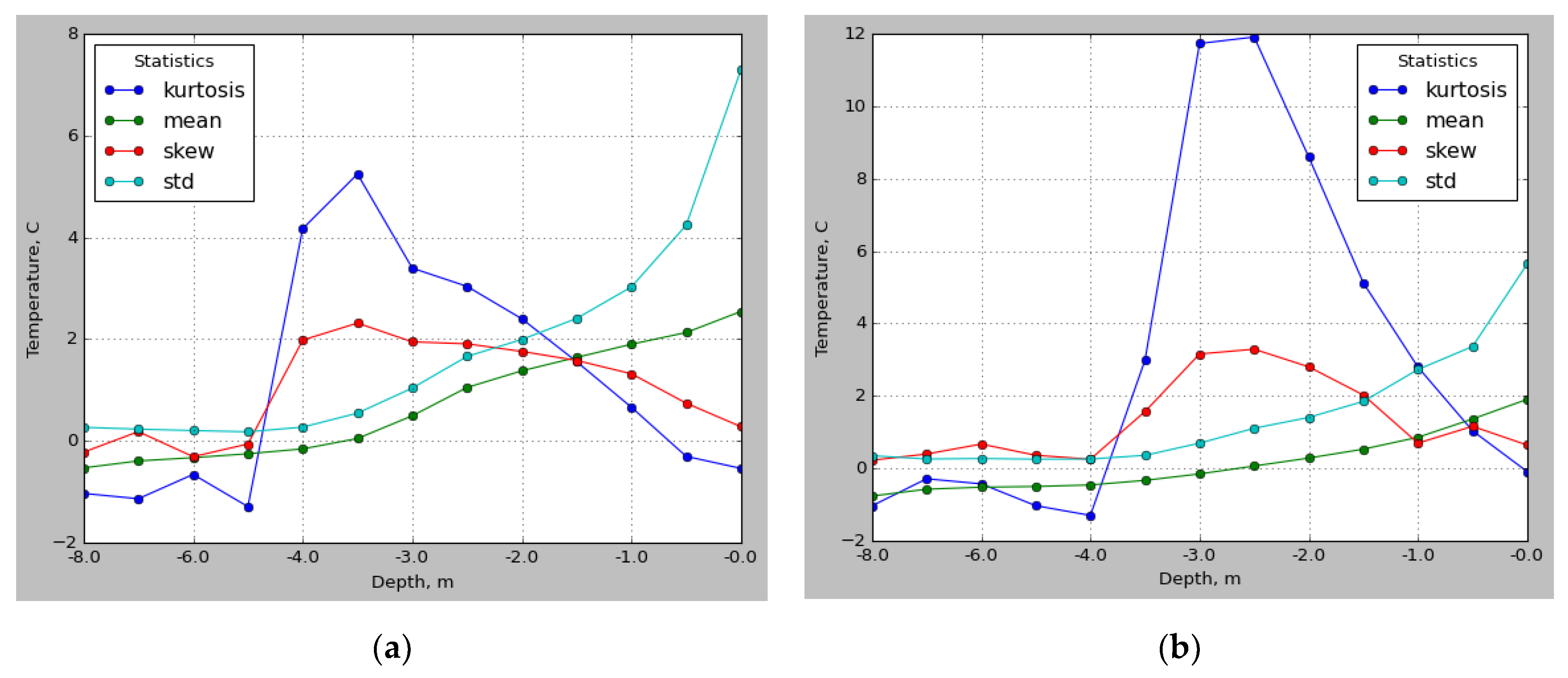
Analysis of the density of temperature measurements at different soil layers defines the transition from a two-top distribution (surface temperatures) to a single-top distribution (medium depth temperature) with a shift in the mathematical expectation towards negative temperatures and a significant decrease in the standard deviation (
Figure 5). Further increase in depth leads to a multi-top distribution. The most significant kurtosis values are at a depth from 3 to 4 m for medium thermowells (
Figure 5a) and from 2 to 3 m for distant thermowells (
Figure 5b).
At the same depths, minor symmetrical distributions are observed. At the same time, the mathematical expectation from layer to layer varies to a lesser extent. The analysis shows that thermal conductivity from depth to depth is a non-stationary process.
2.4. Selecting Uncorrelated Time Series
2.4.1. Linear Correlation
Most methods of incorporating explaining features into a model are based on two opposing principles: their weak mutual correlation or a strong correlation of each feature with a dependent variable [
20]. To assess the linear correlation, we calculated Pearson’s correlation coefficients for temperature measurements at the different depths and distances of the route.
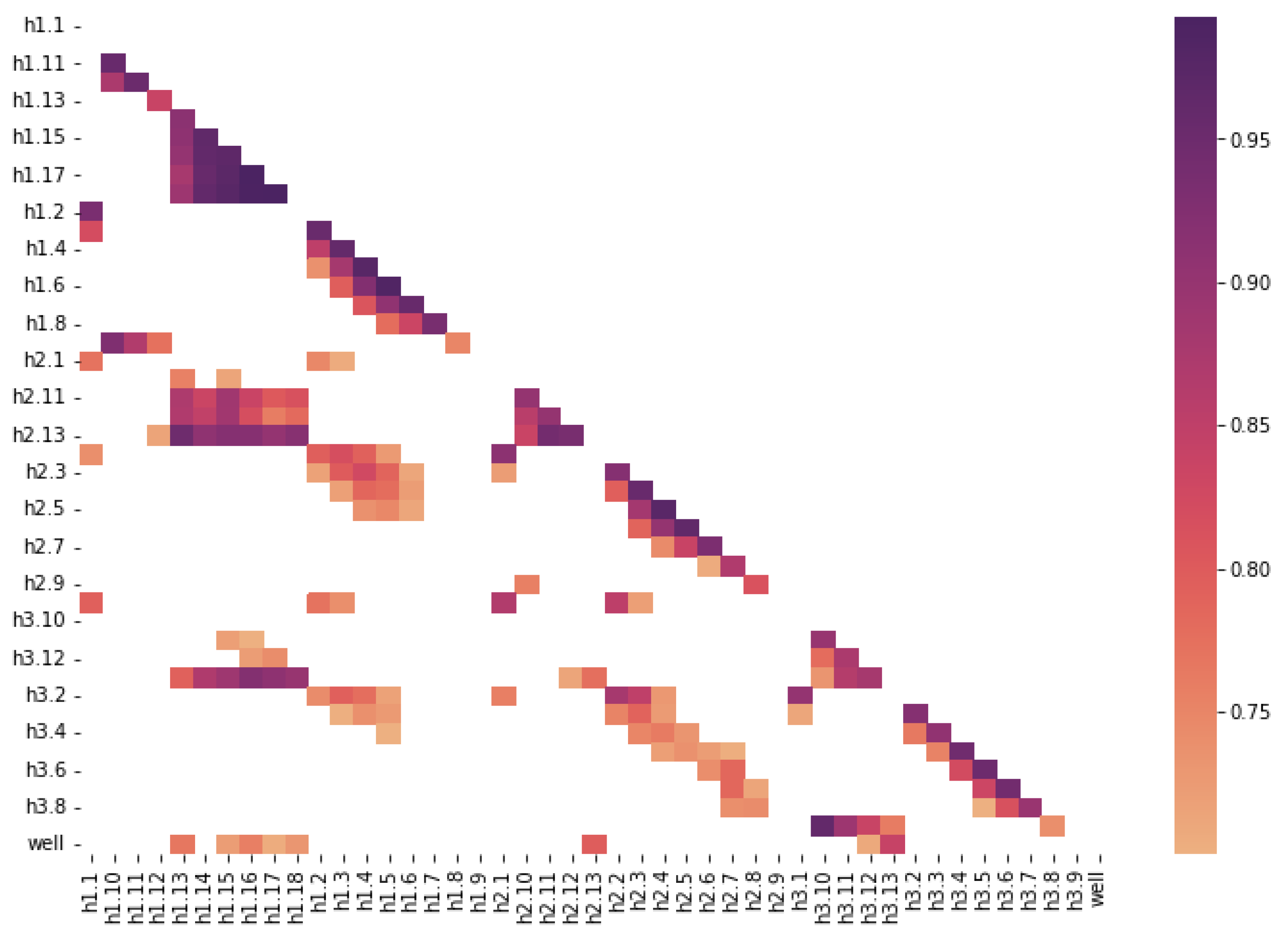
Figure 6 shows the values of Pearson’s linear correlation with a threshold of more than 0.7 per module.
According to the correlation map above, we define a strong correlation between temperature measurements and their locations, for example:
- -
13–18 thermistors of the first line of thermowells (closest to the pipeline),
- -
12–13 thermistors of the second line of thermowells (at the medium distance to the pipeline),
- -
10–13 thermistors of the third line of thermowells (distant from the pipeline).
Because these thermistors are located at depth [5; 13] m, they capture the heating effect of the oil pipeline. At the same time, we define a significant number of highly correlated, layered temperature measurements, such as h1.13–h1.18, h1.3–h1.4–h1.6, and h2.3–h2.5–h2.6. It may indicate the existence of solid geological layers with similar characteristics. The readings of the three surface thermistors h1.1, h2.1, and h3.1 are also positively correlated, so the readings of h1.1 are left for further analysis. As a result of correlation analysis, the measurements on seven thermistors are taken {h1.1, h1.10, h1.14, h1.6, h1.8, h2.7, h3.10}.
2.4.2. Nonlinear Correlation
The publication [
21] suggests the use of Spearman-Kramer correlation coefficients to identify a nonlinear correlation. Spearman’s rank correlation coefficient is a nonparametric measure of rank correlation
:
where
is the covariance of the rank variables,
and are the standard deviations of the rank variables.
Cramer’s correlation coefficient,
φC bases on Pearson’s
χ2 test statistic, and is used for ordinal and binned interval variables:
where
N is the number of observations and
r (
k) is the number of rows (columns) in a contingency table.
To apply nonlinear correlation at the first stage, we convert the existing time feature “Time” of the geotechnical dataset to a set of categorical features that highlights the time difference: a day, a month, a day of a week, or a season of a year (
Table 3), as the moment of measurement impacts the temperature.
Furthermore, in the second stage, we convert the values of linearly uncorrelated features into categorical values using the temperature intervals given in
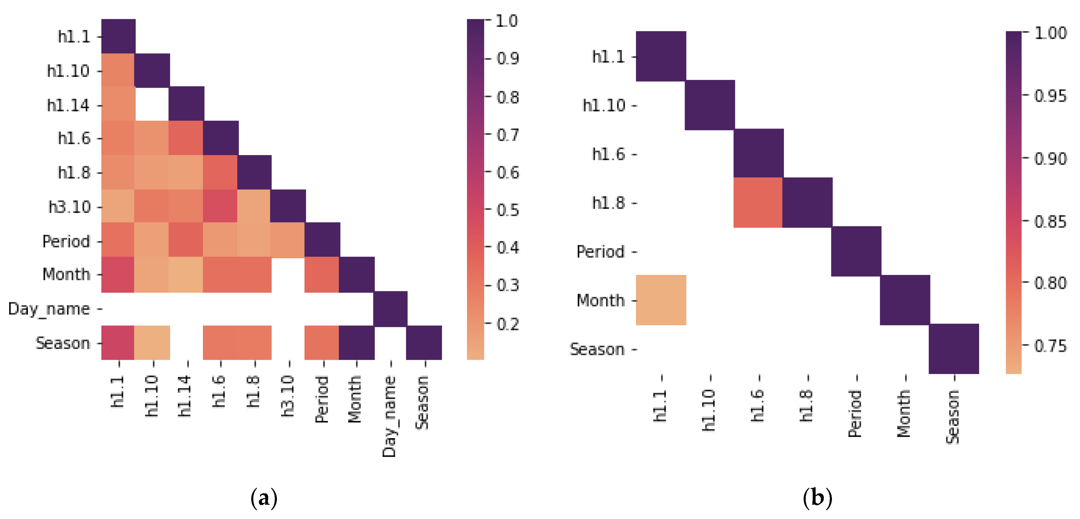
Section 2.3. The resulting categorical data are assessed using a nonlinear relationship between temperature and measurement time (
Figure 7). Colored correlation maps indicate a relationship between layered temperature measurements. The color map of the Cramer correlation coefficients (
Figure 7a) shows that the thermistors h1.14 and h3.10 malfunctioned, and their measurements are indifferent to the days of the week, months and seasons. Therefore, these measurements and the feature named
Day_name are excluded from further analysis. Furthermore, the Spearman correlation matrix (
Figure 7b) establishes the relation between measurements of thermistors h1.6 and h1.8 and correlation between months and temperature fluctuations at the ground surface (thermistors h1.1).
Thus, the resulting set of features appeared as follows {h1.1, h1.6, h1.10, h2.7, Period, Season}.
2.5. Scaling Selected Time Series
To compare temperature measurements at different depths, we apply the robust scaling method because it uses statistics that are robust to outliers:
where
y,
y′ are unscaled and scaled temperature time series;
are the 1st, 2nd, or 3rd quartile of the temperature time series.
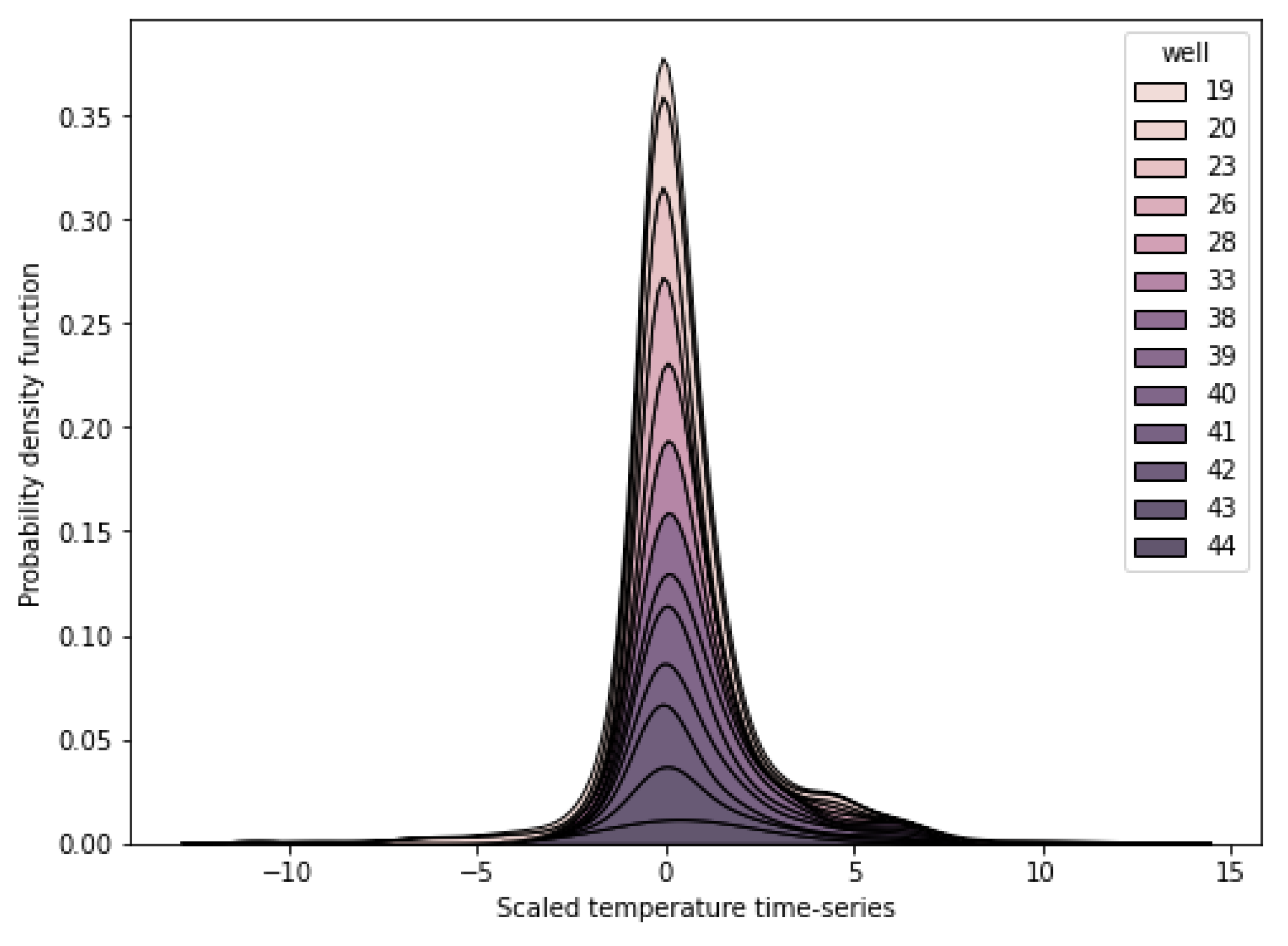
Figure 8 reflects scaled temperature time series grouped according to the thermowells.
Figure 8 shows that probability distributions of scaled temperatures are close to bell-shaped. The height difference of the curves seems to depend on the distance of the thermowell from the heating points.
2.6. Forecasting Model
Smoothing, adaptive, autoregression models, and neural networks can be highlighted among time series forecasting approaches [
1]. We apply a model implemented in the Python library named Facebook Prophet that was opened for users in 2017. Its code is open-sourced and tunable and the result is easy to interpret. The main disadvantages of the model are a requirement for data to be in a specific 2D format (time and temperature) and operating with one-by-one time series. It contains the additive regression model with customizable components:
where
t is time;
is the regression function;
g(t) is the trend component, modeled with piecewise linear, piecewise logistic growth, or flat function;
s(t) is the seasonal component responsible for modeling the periodic changes related to seasonality (seasonality is estimated using a partial Fourier sum);
h(t) is the component responsible for the abnormal days;
is an error that contains information not considered by the model.
3. Results and Discussion
This paper presents the two-step approach to preprocessing sensor data and forecasting soil temperatures. For the first step, temperature analysis is carried out in the following areas: assessing the stability of frozen soils, checking temperature time series for stationarity, elucidating linear and nonlinear relationships between soil layers according to correlation matrices, and bringing the distributions of the temperature series to the bell shape.
It is established that the frozen soils containing the pipeline were mainly in an unstable state with the predominance of the intervals (−2; −0.5] and (−0.5; 1.5] °C.
The statistical analysis of the mathematical expectation and standard deviations shows that thermal conductivity month by month and depth to depth is a non-stationary process.
We define a strong correlation between temperature measurements of the thermistors located at depth [5; 13] m, which means they capture the heating effect of the oil pipeline. Highly correlated temperature measurements, such as h1.13–h1.17, h1.2–h1.6, and h2.1–h2.6, can also indicate the existence of a solid geological layer with similar characteristics.
Reducing temperature time series to dimensionless values by dividing on the difference of the third and first quantiles allows the transformation of the probability density functions to bell curves. All operations were supported with unified scripts in the language Python, which were then integrated into a reproducible workflow.
In the second step we group the transformed dataset around the thermometric wells, the distance to the pipeline and the depth. Then within each group, we split the scaled temperature time series into training and testing samples. The testing sample included the last 90 days of the dataset. Then we applied the training sample for training our model and treated the testing sample as a collection of data points that helped us evaluate whether the model could generalize well to unknown data. Next, we tuned the seasonality component selecting the discretization step at the time grid and calculated and compared accuracy metrics.
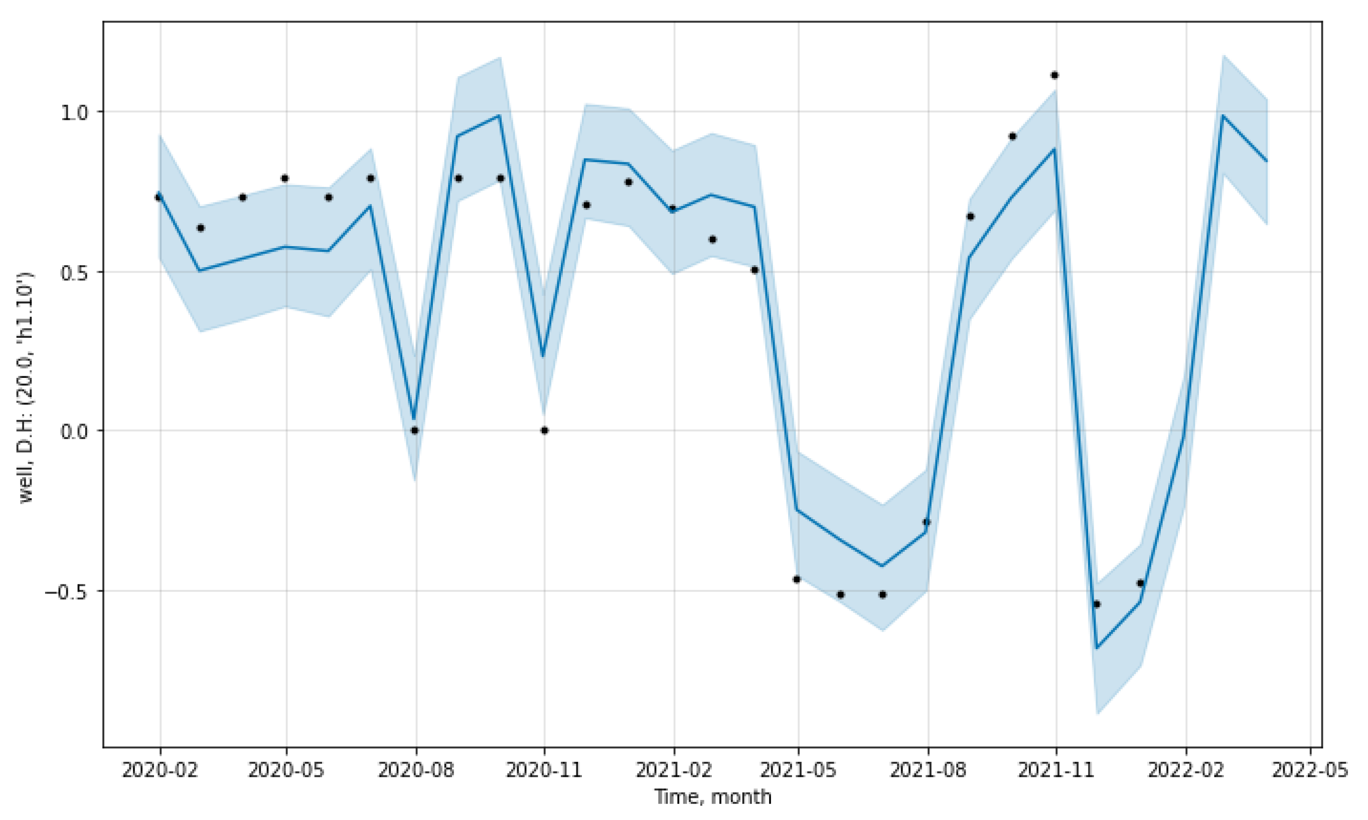
The short-term forecast presented in
Figure 9 is not very favorable, as, by May 2022, the standard deviation of temperature measurements will have increased. The black dots are the actual values, the blue line represents the predicted values, and the blue line is the uncertainty corridor.
This forecast may indicate moderate heat leakage through the joints of pipe sections in the area controlled by the thermometric well no. 20.0.
The forecasting error is assessed using the mean absolute percentage error (MAPE) and the mean square error (MSE) for the temperature measurements. For calculation of the MAPE, actual temperature measurements and their forecast were used:
where
y,
are actual and forecasted temperatures.
With the MAPE, we measured how far the model’s predictions are off from their corresponding outputs on average. The MSE highlights large errors because it squares the difference between actual and forecasted temperatures before summing them:
The lower the MAPE and MSE, the more accurate the prediction. The lowest MAPE and MSE were obtained on the three-month uniform time grid and equaled 24.91% and 0.010, respectively.
The available temperature time series had the following features: incompleteness (11 months), equidistant fixation intervals, non-stationarity, fast-decreasing autocorrelation functions, the range of temperature changes depended on the depth of measurement and the location of a thermowell, as well as the changing trend and the presence of seasonality. The best result, MAE = 34.68% and MSE = 0.043, was given by the forecast on the alternative three-parameter additive Holt–Winters model for a three-week uniform time grid with a seasonality parameter = 15. Holt–Winters forecasting required preliminarily filling the omissions in temperature data by substituting the average group values.
The most effective way to improve the accuracy of machine learning models is to increase the training sample by creating additional features based on the available dataset [
22]. The following can be assumed as additional features: the climatic zones at the sites of the thermowells; the rate of soil erosion; the distance from rivers, roads, and settlements; a detailed characteristic of the terrain; a wind rose; and ravine networks. Separately, it is necessary to note the possibility of overlapping the temperature curve along the pipeline route determined by the locations of points for oil heating.
The additional benefit of the implementation of Facebook Prophet is insensitivity to multiple omissions in data. These omissions appear both in the initial data due to measurement and data transfer failures and in some processing steps, such as when down-discretization was applied to a time grid step.
Further studies of temperature time series can be made in three directions:
designing a digital twin of a pipeline displaying the change in the temperature field of the pipe-to-ground system for three dimensions at once: along the pipe, inland, and at a distance from the pipeline;
integrating temperature changes, soil characteristics, and the location and operation mode of the oil heating points;
retraining a temperature prediction model with new data.
4. Conclusions
A buried pipeline impacts frozen soils when transporting heated oil. Melting permafrost provokes a change in the position of the oil pipeline and can lead to accidents such as an oil spill.
The geotechnical monitoring system that collects soil temperature measurements along the buried oil pipeline includes a significant number of thermowells, a fiber or a wireless network to access local archives, and web servers to process the data.
The thermal influence of a buried pipeline transporting heated oil on frozen soils is uneven and increases during the pipeline’s operation. Preliminary statistical analysis shows that the temperatures of frozen soils containing the oil pipeline are in a high-temperature condition with the predominance of the intervals (−2; −0.5] and (−0.5; 1.5] °C. Collecting volumetric temperature data, the oil operators need a fast, simple, visual, and high-quality method for predicting heat leaks. Higher temperature not associated with seasonality may indicate heat leakage. This study simplifies the forecasting procedure of heat losses along the buried pipeline transporting heated oil.
The proposed approach is express, easily automated, visual, and reasonably accurate to locate and predict heat losses of the buried oil pipeline. It consists of two steps: creation of multidimensional datasets and temperature forecast. The first step includes statistical analysis on a transformed dataset, generation of features sharpened seasonality and permafrost condition, selection of uncorrelated time series, and scaling of the selected time series. The second step is a procedure to forecast time series data based on an additive model where nonlinear trends are fit with yearly, weekly, and daily seasonality.
To generate additional features based on the moment of measurement, the existing time feature is converted to a set of categorical features: a day, a month, a day of a week, and a season of a year. The correlation analysis is implemented with Pearson, Spearman, and Cramer coefficients due to nonlinear temperature–depth and time-series relationships. The amount of the features is decreased by sevenfold. It is established that selecting uncorrelated features reduce the forecasting error. Up-sampling (transition from days to months) and scaling temperature time series convert the probability density function to a bell curve.
The forecasting procedure is provided by the three-component model named Prophet. Prophet fits linear and nonlinear functions to define the trend component and Fourier series to define the seasonal component; the third component, responsible for the abnormal days (when the heating regime is changed for some reason), could be defined by an analyst. Prophet works best with time series with substantial seasonal effects and several seasons of historical data. It is robust against missing data, shifts in the trend, and outliers.
Based upon values of MAPE and MSE (24.91% and 0.010, respectively), it is determined that the most accurate forecast is obtained on a three-month uniform time grid. Reducing the time grid’s step led to the retraining of the model but enlarging it led to an increase in error.


