A Stochastic Multi-Strain SIR Model with Two-Dose Vaccination Rate

Abstract

Infectious diseases remain a substantial public health concern as they are among the leading causes of death. Immunization by vaccination can reduce the infectious diseases-related risk of suffering and death. Many countries have developed COVID-19 vaccines in the past two years to control the COVID-19 pandemic. Due to an urgent need for COVID-19 vaccines, the vaccine administration of COVID-19 is in the mode of emergency use authorization to facilitate the availability and use of vaccines. Therefore, the vaccine development time is extraordinarily short, but administering two doses is generally recommended within a specific time to achieve sufficient protection. However, it may be essential to identify an appropriate interval between two vaccinations. We constructed a stochastic multi-strain SIR model for a two-dose vaccine administration to address this issue. We introduced randomness into this model mainly through the transmission rate parameters. We discussed the uniqueness of the positive solution to the model and presented the conditions for the extinction and persistence of disease. In addition, we explored the optimal cost to improve the epidemic based on two cost functions. The numerical simulations showed that the administration rate of both vaccine doses had a significant effect on disease transmission.

1. Introduction

With a good understanding of the course of the epidemic, we will be in a better position to prevent or monitor communicable diseases, such as Coronavirus Disease 2019 (COVID-19), and to help with the decision making for an effective control strategy. The mathematical epidemic models can forecast the epidemic trajectories and estimate the dynamics of disease transmission and recovery. This information can guide public health practitioners’ responses, offer policymakers a reference for the best allocation of medical resources, and reduce the risk caused by the spread of the epidemic.

Both deterministic and stochastic models have been proposed to model infectious diseases. Modern epidemic models are mostly constructed under the framework of the Susceptible-infected-recovered (SIR) model [1], and most of these models are presented in a deterministic system [2,3,4]. We refer you to [5] for a detailed presentation about the concepts and the related tools for deterministic models. Recently, many articles have introduced stochastic processes to epidemic models. For example, [6,7] brought in random disturbances to the transmission rate of the traditional Susceptible-infected-susceptible (SIS) model. Ref. [8] added random disturbances to the deterministic Susceptible-infected-recovered-susceptible (SIRS) model and explored the impact of intervention strategies. Ref. [9] imported Levy noise in the SIS model.

Quarantine and vaccination are the primary strategies against infectious diseases. Recent studies in the literature have considered models of quarantine [10,11,12,13,14] and have incorporated the social network into models. However, due to the high cost of quarantine, vaccination is among the most effective and long-term approaches. Hence, there is considerable literature discussing infectious disease models with vaccines. For example, [15,16,17] introduced vaccination into SIS models. Ref. [18] discussed the vaccination under the SIR model from the perspective of optimal control. Ref. [19] presented a multi-strain infectious disease model allowing the virus to mutate into a new strain when there is vaccination in the SIR model.

The first reported cases of COVID-19 emerged in 2019 and has infected people around the world. The rapid spread of COVID-19 in the past two years has presented challenges to the international public health and economy. As of 17 April 2022, over 500 million confirmed cases and over six million deaths had been reported globally [20]. Many countries have developed COVID-19 vaccines to prevent the spread of the epidemic. There are several widely known and administered vaccines available on a large scale, including AstraZeneca (AZ), Moderna, Pfizer-BioNTech (BNT), Janssen (Johnson & Johnson), and Sputnik V. Over time, considerable discussions on vaccine-related topics have emerged. For example, [21] presented a systematic review. They provided an overview of clinical data from COVID-19 vaccine development and discussed the strategies to develop vaccines from different infectious diseases, with the aim to aid in developing therapeutic approaches for treatment and prevention of COVID-19. Ref. [22] proposed a new model to discuss the vaccine-resistant issue of COVID-19. Ref. [23] modified the SEIR compartmental model to forecast the possible development of the second COVID-19 wave in European countries. Ref. [24] proposed a multi-regional, hierarchical-tier model for understanding the complexity and heterogeneity of COVID-19 spread and control.

Due to an urgent need for COVID-19 vaccines, the vaccine administration of COVID-19 is in the mode of emergency use authorization requiring less data than typically needed in the early stage. The vaccine development time is therefore extraordinary short; however, to achieve sufficient protection, administering two doses are, in general, recommended within a specific time. Depending on which vaccine was administered, the recommended time-period between doses or the rate of administration may vary.

Therefore, it would be important to obtain an appropriate interval between two vaccinations, which can be then verified through clinical experiment. Recently, [25] proposed an extended SEAIRD compartmental model to describe the epidemic dynamics with both single-dose and double-dose vaccine administrations. They utilized the deterministic framework of nonlinear constrained optimal control problems to solve optimal vaccine administration problems. In addition, they only focused on the scenario with only one strain, which does not resemble reality. In this study, we hope to conduct a broader discussion on vaccination frequency through the construction of mathematical models. Additionally, due to a fast-spreading and higher mutation rate of the virus, there is already evidence to have more than one mutated strain of the new coronavirus. To take these into consideration, we will therefore construct a stochastic, multi-strain SIR model for a two-dose vaccine.

We structure the rest of this paper as follows. Section 2 presents the reasoning of our model and discusses its basic properties, such as equilibrium points and basic reproduction numbers of the deterministic model. Section 3 then focuses on its properties associated with the main stochastic model. Some numerical examples are shown to illustrate the results of our model in Section 4. We conclude this work in Section 5.

2. The Model

Table 1 lists the variables and parameters of our model.

Table 1. Description of variables and parameters in model (1).

Variable/Parameter	Description
$S\left(t\right)$	$\mathrm{the} \mathrm{number} \mathrm{of} \mathrm{susceptible} \mathrm{individuals} \mathrm{at} \mathrm{time} t$
$I_k\left(t\right)$	$\mathrm{the} \mathrm{number} \mathrm{of} \mathrm{infectious} \mathrm{individuals} \mathrm{at} \mathrm{time} t \mathrm{who} \mathrm{were} \mathrm{infected} \mathrm{by} \mathrm{strain} k$
$R\left(t\right)$	$\mathrm{the} \mathrm{number} \mathrm{of} \mathrm{recovered} \mathrm{individuals} \mathrm{at} \mathrm{time} t$
$V_i\left(t\right)$	$\mathrm{the} \mathrm{number} \mathrm{of} \mathrm{individuals} \mathrm{who} \mathrm{received} \mathrm{the} i\mathrm{th} \mathrm{dose} \mathrm{of} \mathrm{the} \mathrm{vaccine} \mathrm{at} \mathrm{time} t$
$b$	the birth rate
${\beta }_k$	$\mathrm{the} \mathrm{transmission} \mathrm{rate} \mathrm{of} \mathrm{strain} k$
${\gamma }_k$	$\mathrm{the} \mathrm{recovery} \mathrm{rate} \mathrm{of} \mathrm{strain} k$
$\delta$	the rate at which immunity disappears in recovered individuals
$q_0$	the vaccination rate of the first dose among susceptible individuals
$q_1$	the vaccination rate of the second dose among individuals who received first dose of vaccine
${\epsilon }_1$	the rate at which immunity disappears among susceptible individuals receiving 1 dose of vaccine
${\epsilon }_2$	the rate at which immunity disappears among susceptible individuals receiving 2 doses of vaccine
${\mu }_k$	$\mathrm{the} \mathrm{death} \mathrm{rate} \mathrm{due} \mathrm{to} \mathrm{strain} k$
${\mu }_N$	the natural death rate

We consider a multi-strain SIR model as shown in (1). We assume that there are $K$ types of strain and only one single vaccine available. The model includes susceptible population ($S$), the number of individuals who received only one dose of the vaccine ($V_1$), the number of individuals who received two doses of the vaccine ($V_2$), the number of people infected by the kth strain ($I_k$), and the number of individuals who were recovered ($R$). We assume that each susceptible person is infected with at most a single strain at a time. We present their relationship between the compartments in Figure 1, and introduce the following proposed model

$$\{\begin{array}{l}dS\left(t\right)=\left[b-S\left(t\right){\displaystyle {\displaystyle \sum }_{k=1}^K}{\beta }_k{I}_k\left(t\right)-\left({\mu }_N+q_0\right)S\left(t\right)+{\displaystyle {\displaystyle \sum }_{i=1}^2}{\epsilon }_i{V}_i\left(t\right)+\delta R\left(t\right)\right]dt,\\ d{I}_k\left(t\right)=\left[{\beta }_{k}S\left(t\right)I_k\left(t\right)-\left({\mu }_N+{\mu }_k+{\gamma }_k\right)I_k\left(t\right)\right]dt, k=1,2,\dots ,K,\\ dR\left(t\right)=\left[{\displaystyle {\displaystyle \sum }_{k=1}^K}{\gamma }_k{I}_k\left(t\right)-\left({\mu }_N+\delta \right)R\left(t\right)\right]dt,\\ d{V}_1\left(t\right)=\left[q_{0}S\left(t\right)-\left({\mu }_N+{\epsilon }_1+q_1\right)V_1\left(t\right)\right]dt,\\ d{V}_2\left(t\right)=\left[q_1{V}_1\left(t\right)-\left({\mu }_N+{\epsilon }_2\right)V_2\left(t\right)\right]dt.\end{array}$$

(1)

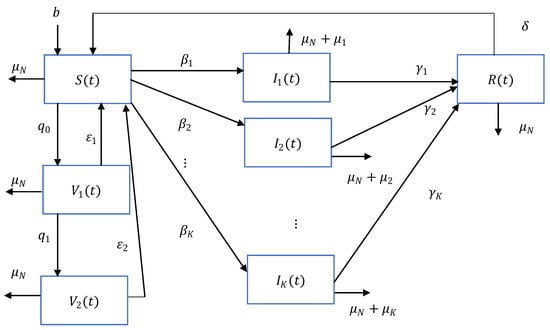
Figure 1. Compartment diagram for the proposed multi-strain SIR model.

We assume that the vaccine has a complete anti-epidemic effect on each strain, but its effect will disappear at a certain rate, returning the vaccinated person to the situation before the vaccination. Although this is different from reality, it may approximate the ineffectiveness of the vaccine against different strains.

Suppose that the number of total populations is $N\left(t\right)=S\left(t\right)+{\sum }_{k=1}^K{I}_k\left(t\right)+{\sum }_{i=1}^2{V}_i\left(t\right)+R\left(t\right)$. It implies

$$\begin{array}{l}d\left[S\left(t\right)+{\sum }_{k=1}^K{I}_k\left(t\right)+R\left(t\right)+{\sum }_{i=1}^2{V}_i\left(t\right)\right]\\ =\left[b-{\mu }_{N}N\left(t\right)-{\displaystyle {\displaystyle \sum }_{k=1}^K}{\mu }_k{I}_k\left(t\right)\right]dt\le \left[b-{\mu }_{N}N\left(t\right)\right]dt\end{array}$$

(2)

Then, we have $N\left(t\right)\le N_1$, $\forall t\ge 0$, where

$$N_1=\{\begin{array}{c}\frac{b}{{\mu }_N},\hspace{1em}\mathrm{if} N\left(0\right)\le \frac{b}{{\mu }_N};\\ N\left(0\right), \mathrm{if} N\left(0\right)>\frac{b}{{\mu }_N}.\end{array}$$

(3)

To simplify the following discussion, we assume $N\left(0\right)\le \frac{b}{{\mu }_N}$. Next, we will discuss the stability of model (1) on an invariant set $\mathsf{\Lambda }$:

$$\mathsf{\Lambda }=\left\{\theta =\left({\theta }_1,\dots ,{\theta }_{K+4}\right)\in {ℝ}_{+}^{K+4}|{\sum }_{k=1}^{K+4}{\theta }_k\le \frac{b}{{\mu }_N}\right\},$$

(4)

where ${\theta }_1=S$, $\left({\theta }_2,\dots ,{\theta }_{K+1}\right)=I=\left(I_1,\dots ,I_K\right)$, ${\theta }_{K+2}=R$, $\left({\theta }_{K+3},{\theta }_{K+4}\right)=V=\left(V_1,V_2\right)$.

2.1. The Equilibrium Point and the Basic Reproduction Number

We have some equilibrium points of our model on $\mathsf{\Lambda }$, and its first point is the disease-free equilibrium point $P^0=\left(S^0,I_1^0,\dots ,I_k^0,R^0,V_1^0,V_2^0\right)$, where

$$\{\begin{array}{l}{S}^0=\frac{b}{{\mu }_N}\frac{\left({\mu }_N+{\epsilon }_2\right)\left({\mu }_N+{\epsilon }_1+q_1\right)}{\left({\mu }_N+{\epsilon }_2\right)\left({\mu }_N+{\epsilon }_1+q_1\right)+q_0\left({\mu }_N+{\epsilon }_2\right)+q_0{q}_1},\\ V_1^0=\frac{b}{{\mu }_N}\frac{q_0\left({\mu }_N+{\epsilon }_2\right)}{{\mu }_N^2+{\mu }_N\left({\epsilon }_2+{\epsilon }_1+q_0+q_1\right)+\left(q_0{\epsilon }_2+q_1{\epsilon }_2+q_0{q}_1+{\epsilon }_1{\epsilon }_2\right)},\\ V_2^0=\frac{b}{{\mu }_N}\frac{q_0{q}_1}{{\mu }_N^2+{\mu }_N\left({\epsilon }_2+{\epsilon }_1+q_0+q_1\right)+\left(q_0{\epsilon }_2+q_1{\epsilon }_2+q_0{q}_1+{\epsilon }_1{\epsilon }_2\right)},\\ I_1^0=I_2^0=\cdots =I_K^0=R^0=0.\end{array}$$

(5)

If the number of infected people is positive only for strain $k$ and the rest is 0, the endemic equilibrium point is $P_k^{*}=\left(S^{*},{\tilde{I}}_k^{*},R^{*},V_1^{*},V_2^{*}\right)$, and

$$\{\begin{array}{l}{S}^{*}=\frac{{\mu }_N+{\mu }_k+{\gamma }_k}{{\beta }_k},\\ V_1^{*}=\frac{q_0\left({\mu }_N+{\mu }_k+{\gamma }_k\right)}{{\beta }_{0k}\left({\mu }_N+{\epsilon }_1+q_1\right)},\\ V_2^{*}=\frac{q_0{q}_1\left({\mu }_N+{\mu }_k+{\gamma }_k\right)}{{\beta }_k\left({\mu }_N+{\epsilon }_1+q_1\right)\left({\mu }_N+{\epsilon }_2\right)},\\ R^{*}=\frac{{\gamma }_k{I}_k^{*}}{{\mu }_N+\delta },\\ I_k^{*}=\frac{b{\beta }_k\left({\mu }_N+{\epsilon }_1+q_1\right)\left({\mu }_N+{\epsilon }_2\right)-{\mu }_N\left({\mu }_N+{\mu }_k+{\gamma }_k\right)\left[{\mu }_N^2+{\mu }_N{\epsilon }_2+q_0{q}_1\right]}{{\beta }_k\left({\mu }_N+{\epsilon }_1+q_1\right)\left({\mu }_N+{\epsilon }_2\right)\left({\mu }_N+{\mu }_k+{\gamma }_k-{\gamma }_k/\left({\mu }_N+\delta \right)\right)}\end{array}$$

(6)

$k=1,2,\dots ,K$. Note that ${\tilde{I}}_k^{*}=\left(I_1^{*},\dots ,I_K^{*}\right)$ means $I_k^{*}>0$ and $I_l^{*}=0, \forall l\ne k$.

Using the next generation method, we can obtain the basic reproduction number.

Set

$$F=\mathrm{diag}\left({\beta }_{1}S,\dots {\beta }_{K}S\right)$$

(7)

and

$$V=\mathrm{diag}\left({\mu }_N+{\mu }_1+{\gamma }_1,\dots {\mu }_N+{\mu }_K+{\gamma }_K\right)$$

(8)

The next generation matrix is

$$F{V}^{-1}=\mathrm{diag}\left(\frac{{\beta }_{k}S}{{\mu }_N+{\mu }_k+{\gamma }_k},k=1,2,\dots ,K\right)$$

(9)

Substituting $S$ with $S^0$, we have the basic reproduction number $R_{0k}=\frac{{\beta }_k{S}^0}{{\mu }_N+{\mu }_k+{\gamma }_k}$ for strain $k$ in the deterministic model, that is,

$$R_{0k}:=\frac{b}{{\mu }_N}\frac{{\beta }_k\left({\mu }_N+{\epsilon }_1+q_1\right)\left({\mu }_N+{\epsilon }_2\right)}{\left({\mu }_N+{\mu }_k+{\gamma }_k\right)\left[\left({\mu }_N+{\epsilon }_1+q_1\right)\left({\mu }_N+{\epsilon }_2\right)+q_0\left({\mu }_N+{\epsilon }_2\right)+q_0{q}_1\right]},$$

(10)

$k=1,2,\dots ,K$. This yields the basic reproduction number of model (1) with

$$R_0=\max \left\{R_{0k},k=1,2,\dots ,K\right\}$$

(11)

2.2. Sensitivity Analysis of the Basic Reproduction Number to Parameters

Sensitivity analysis can be used to explore the effect on outcomes due to the changes in each parameter within a specified range in a mathematical model. In the studies of [26,27], the LHS/PRCC (Latin hypercube sampling/partial rank correlation coefficients) technique was used to analyze the sensitivity of parameters in $R_0$. In this subsection, we use the same technique to find the parameters that have more influence on $R_0$.

First, we set the probability functions of the parameters. We assign the birth rate $b$ to have a uniform distribution between 0 and 5, and denote it as $b$~U(0, 5). Except for ${\epsilon }_2$, we set the rest of the parameters to have uniform distributions between 0 and 1. We assume to have a lower vaccine failure rate after two doses of the vaccine, and hence, ${\epsilon }_2$ < ${\epsilon }_1$. We set ${\epsilon }_2$~U (0, ${\epsilon }_1$).

There are 3K + 7 parameters in model (1), and we set the number of simulations to 1000 times. In other words, we generate a 1000 × (3K + 7) LHS table as the input matrix and use $R_0$as the output variable. Next, we calculate the PRCCs and test whether the coefficients are 0′s. We use the lhs package in R to generate the LHS table and use the sensitivity package to test the PRCCs. Note that the bootstrap method with repeated sampling 2000 times is used. The results with K = 3 are shown in Table 2 and Figure 2.

Table 2. Partial rank correlation coefficients.

Parameter	PRCC	Parameter	PRCC
$b$	0.8258 **	${\gamma }_2$	−0.1198 **
${\beta }_1$	0.3185 **	${\gamma }_3$	−0.1515 **
${\beta }_2$	0.2817 **	${\mu }_1$	−0.2133 **
${\beta }_3$	0.2523 **	${\mu }_2$	−0.1224 **
$\delta$	−0.0699 *	${\mu }_3$	−0.0917 **
${\epsilon }_1$	0.0530	${\mu }_N$	−0.8421 **
${\epsilon }_2$	0.1044 **	$q_0$	−0.3632 **
${\gamma }_1$	−0.1843 **	$q_1$	−0.0481

The results are significant at the 0.05 level (*) or the 0.01 level (**).

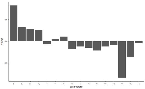
Figure 2. Significance test of 3-train model parameters and PRCC results for $R_0$.

Except for ${\epsilon }_1$ and $q_1$, other parameters are significant, but these two parameters are directly related to $q_0$ and ${\epsilon }_2$. Both $q_0$ and $q_1$ are negatively correlated with $R_0$, that is, the higher the vaccination rate, the smaller the $R_0$. This is in line with the hypothesis that vaccines inhibit disease transmission. Conversely, ${\epsilon }_1$ and ${\epsilon }_2$ represent vaccine failure rates, which are positively correlated with $R_0$. The most sensitive parameters are b and ${\mu }_N$. The ratio $b/{\mu }_N$ represents the upper limit of the population. From Equation (5), this ratio has a definite linear relationship with the value of $R_0$.

2.3. The Stochastic Model

Following the spirit of the model in [6], we assume that the disease transmission rates fluctuate around some average values. Let $\left(\mathsf{\Omega },ℱ,{\left\{{ℱ}_t\right\}}_{t\ge 0},P\right)$ be a complete probability space, and ${\beta }_k~{\beta }_{0k}+{\sigma }_{k}d{B}_k\left(t\right)$, where $B_k$ are independent standard Brownian motions, ${\beta }_{0k}$ is the expected value of ${\beta }_k$, and ${\sigma }_k$ are the amplitudes of ${\beta }_k$, $k=1,2,\dots ,K$. Thus, the proposed stochastic model becomes

$$\{\begin{array}{l}dS\left(t\right)=\left[b-S{\displaystyle {\displaystyle \sum }_{k=1}^K}{\beta }_{0k}{I}_k-\left({\mu }_N+q_0\right)S+{\displaystyle {\displaystyle \sum }_{i=1}^2}{\epsilon }_i{V}_i+\delta R\right]dt-S{\displaystyle {\displaystyle \sum }_{k=1}^K}{\sigma }_k{I}_{k}d{B}_k\left(t\right),\\ d{I}_k\left(t\right)=\left[{\beta }_{0k}S{I}_k-\left({\mu }_N+{\mu }_k+{\gamma }_k\right)I_k\right]dt+{\sigma }_{k}S{I}_{k}d{B}_k\left(t\right), k=1,2,\dots ,K,\\ dR\left(t\right)=\left[{\displaystyle {\displaystyle \sum }_{k=1}^K}{\gamma }_k{I}_k-\left({\mu }_N+\delta \right)R\right]dt,\\ d{V}_1\left(t\right)=\left[q_{0}S-\left({\mu }_N+{\epsilon }_1+q_1\right)V_1\right]dt,\\ d{V}_2\left(t\right)=\left[q_1{V}_1-\left({\mu }_N+{\epsilon }_2\right)V_2\right]dt.\end{array}$$

(12)

Note that model (12) is generalized from SIR or can be seen as a special case of the SVIRS model [28]. However, unlike the previous articles, we considered the impact of two vaccine doses on the epidemic under multi-strain infectious diseases.

3. The Asymptotic Behavior of the Stochastic Model

In this section, we study the mathematical properties of the model (12).

3.1. Existence of Unique Positive Solution

In Theorem 1, we show that there is a unique global and positive solution of model (12). That is, $\mathsf{\Lambda }$ is the positive invariant set of model (12) with probability 1.

Theorem 1.

Given arbitrary initial vector $\theta \left(0\right)\in \mathsf{\Lambda }$, model (12) has a unique positive solution $\theta \left(t\right)\in \Lambda$for all$t\ge 0$with probability 1. That is,

$$P\left(\theta \left(t\right)\in \mathsf{\Lambda }, \forall t\ge 0\right)=1.$$

(13)

Proof. 

See Appendix A. □

3.2. Extinction

The threshold for the disappearance of the disease is an important property for the epidemic model. We define the basic reproductive number for each strain as

$$R_{0k}^S:=R_{0k}-\frac{{\sigma }_k^2}{2\left({\mu }_N+{\mu }_k+{\gamma }_k\right)}{\left(S^0\right)}^2,$$

(14)

$k=1,2,\dots ,K$. The basic reproductive number for model (12) is

$$R_0^S:=\max \left\{R_{0k}^S, k=1,2,\dots ,K\right\}.$$

(15)

To facilitate subsequent discussions, we define

$$x_t={⟨x⟩}_t=\frac{1}{t}{\int }_0^{t}x\left(s\right)ds \mathrm{and} {⟨x,x⟩}_t=\frac{1}{t}{\int }_0^t{x}^2\left(s\right)ds.$$

(16)

The following lemma is useful for our discussion.

Lemma 1

(Strong Law of Large Numbers [29]). Let $M={\left\{M_t\right\}}_{t\ge 0}$ be a real-valued continuous local martingale vanishing at $t=0$ . Then

$$\underset{t\to \infty }{\lim }{⟨M,M⟩}_t=\infty , a.s. \Rightarrow \underset{t\to \infty }{\lim }\frac{M_t}{{⟨M,M⟩}_t}=0, a.s.$$

(17)

and also

$$\underset{t\to \infty }{\mathrm{limsup}}\frac{{⟨M,M⟩}_t}{t}<\infty , a.s. \Rightarrow \underset{t\to \infty }{\lim }\frac{M_t}{t}=0, a.s.$$

(18)

Theorem 2.

In model (12), consider the following two conditions:

(a)

$R_{0k}^S=R_{0k}-\frac{{\sigma }_k^2}{2\left({\mu }_N+{\mu }_k+{\gamma }_k\right)}{\left(S^0\right)}^2<1$ and ${\beta }_{0k}>S^0{\sigma }_k^2$, or

(b)

$\frac{{\beta }_{0k}^2}{2\left({\mu }_N+{\mu }_k+{\gamma }_k\right)}<{\sigma }_k^2$.

If one of the above conditions holds, then for an arbitrary initial vector $\theta \left(0\right)\in \mathsf{\Lambda }$, the solution$\theta \left(t\right)\in \mathsf{\Lambda }$ obeys

$$\underset{t\to \infty }{\mathrm{limsup}}\frac{\ln I_k\left(t\right)}{t}<0, a.s.$$

(19)

In other words, the number of infectious individuals infected by the kth strain, $I_k$, tends to zero exponentially with probability 1 for $k=1,2,\dots ,K$.

Proof. 

See Appendix B. □

Remark 1.

The condition (b) of Theorem 2 implies $R_{0k}^S<1$. As we can express $R_{0k}^S$ as a function of$S^0$, we have

$$f\left(S^0\right):=R_{0k}^S=\frac{{\beta }_{0k}{S}^0}{\left({\mu }_N+{\mu }_k+{\gamma }_k\right)}-\frac{{\sigma }_k^2}{2\left({\mu }_N+{\mu }_k+{\gamma }_k\right)}{\left(S^0\right)}^2.$$

(20)

Note that $f\left(\frac{{\beta }_{0k}}{{\sigma }_k^2}\right)=\frac{{\beta }_{0k}^2}{2\left({\mu }_N+{\mu }_k+{\gamma }_k\right){\sigma }_k^2}$ is the maximum of $f$. Then, $\frac{{\beta }_{0k}^2}{2\left({\mu }_N+{\mu }_k+{\gamma }_k\right)}<{\sigma }_k^2$ implies$R_{0k}^S<1$. That is, we can rewrite Theorem 2 as the following Theorem 3.

Theorem 3.

In model (12), consider the following two conditions:

(a)

$R_{0k}^S=R_{0k}-\frac{{\sigma }_k^2}{2\left({\mu }_N+{\mu }_k+{\gamma }_k\right)}{\left(S^0\right)}^2<1$ and ${\beta }_{0k}>S^0{\sigma }_k^2$, or

(b)

$\frac{{\beta }_{0k}^2}{2\left({\mu }_N+{\mu }_k+{\gamma }_k\right)}<{\sigma }_k^2$,

If one of the above conditions holds,then for arbitrary initial vector $\theta \left(0\right)\in \mathsf{\Lambda }$, the solution$\theta \left(t\right)\in \mathsf{\Lambda }$ obeys $\underset{t\to \infty }{\mathrm{limsup}}\frac{\ln I_k\left(t\right)}{t}<0, a.s.$

That is,$I_k$tends to zero exponentially with probability 1 for $k=1,2,\dots ,K$.

3.3. Persistence

In this subsection, we discuss the persistence of the disease. In this paper, we call a disease persistent if $\underset{t\to \infty }{\mathrm{liminf}}{\sum }_{k=1}^K{I}_k>0, a.s.$ holds. We define

$$R_{0k}^{*}:=R_{0k}-\frac{{\sigma }_k^2}{2\left({\mu }_N+{\mu }_k+{\gamma }_k\right)}{\left(\frac{b}{{\mu }_N}\right)}^2,$$

(21)

$k=1,2,\dots ,K$. As $R_{0k}^{*}\le R_{0k}^S$, $R_{0k}^{*}>1$ implies $R_{0k}^S>1$.

Theorem 4.

For arbitrary initial vector $\theta \left(0\right)\in \mathsf{\Lambda }$,

(a)

If$\max \left\{R_{0k}^{*}\right\}>1$, we have

$$\underset{t\to \infty }{\mathrm{liminf}}{\sum }_{k=1}^K{I}_k{}_t\ge \underset{\_}{\xi }:=\frac{({\mu }_N+{\mu }_{{\widehat{k}}^{*}}+{\gamma }_{{\widehat{k}}^{*}})\left(R_{0{\widehat{k}}^{*}}^{*}-1\right)}{{\beta }_{0{\widehat{k}}^{*}}\frac{S^0}{b}\left(({\mu }_N+{\mu }_{{\tilde{k}}^{*}}+{\gamma }_{{\tilde{k}}^{*}})-\frac{\delta {\gamma }_{{\tilde{k}}^{*}}}{{\mu }_N+\delta }\right)} a.s.,$$

(22)

where ${\tilde{k}}^{*}=\underset{k:R_{0k}^{*}>1}{\arg \max }\left\{\left({\mu }_N+{\mu }_k+{\gamma }_k\right)-\frac{\delta {\gamma }_k}{{\mu }_N+\delta }\right\}$ and ${\widehat{k}}^{*}=\underset{k:R_{0k}^{*}>1}{\arg \max }\left\{\frac{\left({\mu }_N+{\mu }_k+{\gamma }_k\right)\left(R_{0k}^{*}-1\right)}{{\beta }_{0k}}\right\}$.

(b)

If there are some persistent strains with ${\beta }_{0k_0}>S^0{\sigma }_{k_0}^2$ and $R_{0k_0}^{*}>1$, then

$$\underset{t\to \infty }{\mathrm{limsup}}{\sum }_{k=1}^K⟨I_k⟩{}_t\le \overline{\xi }:=\frac{\left({\mu }_N+{\mu }_{{\widehat{k}}_0}+{\gamma }_{{\widehat{k}}_0}\right)\left(R_{0{\widehat{k}}_0}^S-1\right)}{({\beta }_{0{\widehat{k}}_0}-S^0{\sigma }_{{\widehat{k}}_0}^2)\frac{S^0}{b}\left(({\mu }_N+{\mu }_{{\tilde{k}}_{*}}+{\gamma }_{{\tilde{k}}_{*}})-\frac{\delta {\gamma }_{{\tilde{k}}_{*}}}{{\mu }_N+\delta }\right)} a.s.,$$

(23)

where${\tilde{k}}_{*}=\underset{k:R_{0k}^{*}>1}{\arg \min }\left\{\left({\mu }_N+{\mu }_k+{\gamma }_k\right)-\frac{\delta {\gamma }_k}{{\mu }_N+\delta }\right\}$and${\widehat{k}}_0=\underset{k_0:R_{0k_0}^S>1}{arg max}\left\{\frac{\left({\mu }_N+{\mu }_{k_0}+{\gamma }_{k_0}\right)\left(R_{0k_0}^S-1\right)}{\left({\beta }_{0k_0}-S^0{\sigma }_{k_0}^2\right)}\right\}$.

Proof. 

See Appendix C. □

From Theorem 4, the value of ${\sum }_{k=1}^K⟨I_k⟩{}_t$ should oscillate in the interval $\left[\underset{\_}{\xi },\overline{\xi }\right]$ if $t$ is large enough. That is, some strains will persist, and after a certain period of time $t$, the average number of infected people will stay in this interval. We next discuss the conditions for the extinction or existence of the strains. Define

$${\overline{k}}^{*}=\arg {\max }_{k:R_{0k}^S>1}{R}_{0k}^S.$$

(24)

Then, it is obvious that $R_{0{\overline{k}}^{*}}^S=R_0^S$. We prove that, under specified conditions, strain ${\overline{k}}^{*}$ is the uniquely persistent strain in Theorem 4.

Theorem 5.

Suppose the conditions of Theorem 4 all hold. Assume that

$$\underset{t\to \infty }{\lim }\frac{\ln I_{{\overline{k}}^{*}}\left(t\right)-\ln I_{{\overline{k}}^{*}}\left(0\right)}{t}=0, a.s.$$

(25)

and there are some $k\ne {\overline{k}}^{*}$ with $R_{0{\overline{k}}^{*}}^S>R_{0k}^S>1$. If

(a)

$\frac{{\beta }_{0{\overline{k}}^{*}}}{{\sigma }_{{\overline{k}}^{*}}^2}\ge \frac{{\beta }_{0k}}{{\sigma }_k^2}$ and $\frac{{\sigma }_{{\overline{k}}^{*}}^2}{\left({\mu }_N+{\mu }_{{\overline{k}}^{*}}+{\gamma }_{{\overline{k}}^{*}}\right)}>\frac{{\sigma }_k^2}{\left({\mu }_N+{\mu }_k+{\gamma }_k\right)}$, or

(b)

$\frac{{\beta }_{0{\overline{k}}^{*}}}{{\sigma }_{{\overline{k}}^{*}}^2}<\frac{{\beta }_{0k}}{{\sigma }_k^2}$ and $\frac{{\sigma }_k^2}{\left({\mu }_N+{\mu }_k+{\gamma }_k\right)}>\left(\frac{R_{0k}^S-1}{R_{0{\overline{k}}^{*}}^S-1}\right)\frac{{\sigma }_{{\overline{k}}^{*}}^2}{\left({\mu }_N+{\mu }_{{\overline{k}}^{*}}+{\gamma }_{{\overline{k}}^{*}}\right)}$,

we have $\underset{t\to \infty }{\mathrm{limsup}}\frac{\ln I_k\left(t\right)-\ln I_k\left(0\right)}{t}<0, a.s.$, i.e., $\underset{t\to \infty }{\lim }{I}_k\left(t\right)=0, a.s.$

Proof. 

See Appendix D. □

3.4. Vaccination Rates

In this subsection, we discuss the utilities of the proposed model. This model treats vaccination as the primary disease preventative approach, and the relevant parameters in the model are the two-dose vaccination rates $q_0$ and $q_1$. Using Equation (5) and letting $A=\frac{b}{{\mu }_N}, B={\mu }_N^2+{\mu }_N\left({\epsilon }_2+{\epsilon }_1\right)+{\epsilon }_1{\epsilon }_2$, and $C={\epsilon }_2+{\mu }_N$, then

$$S^0=A\frac{B+q_1\left({\epsilon }_2+{\mu }_N\right)}{B+q_1\left({\epsilon }_2+{\mu }_N\right)+q_0\left({\epsilon }_2+{\mu }_N\right)+q_0{q}_1}=A\frac{B^{\prime }+q_1}{B^{\prime }+q_1+q_0+q_1{q}_0/C},$$

(26)

where $B^{\prime }=\frac{B}{C}=\frac{{\mu }_N^2+{\mu }_N\left({\epsilon }_2+{\epsilon }_1\right)+{\epsilon }_1{\epsilon }_2}{{\epsilon }_2+{\mu }_N}={\mu }_N+{\epsilon }_1$. As people who have received their first dose of the vaccine are often more willing to take a second dose, we can simplify the assumptions of model (12). For example, we set $q_0=q_1^2$, then $S^0=A\frac{B^{\prime }+q_1}{B^{\prime }+q_1+q_1^2+q_1^3/C}$, and

$$\frac{\partial S^0}{\partial q_1}=A\left(\frac{1}{B^{\prime }+q_1+q_1^2+\frac{a{q}_1^3}{C}}-\frac{\left(B^{\prime }+q_1\right)(1+2q_1+3\frac{q_1^2}{C})}{{\left(B^{\prime }+q_1+q_1^2+\frac{q_1^3}{C}\right)}^2}\right)=-A\left(\frac{2B^{\prime }{q}_1+\left(\frac{3B^{\prime }}{C}+1\right)q_1^2+\frac{2q_1^3}{C}}{{\left(B^{\prime }+q_1+q_1^2+\frac{q_1^3}{C}\right)}^2}\right)<0.$$

(27)

As discussed in Remark 1, $R_{0k}^S$ has a global maximum at $S^0=\frac{{\beta }_{0k}}{{\sigma }_k^2}$. It implies that if ${\beta }_k>{\sigma }_k^2{S}^0$, $R_{0k}^S$ is an increasing function of $S^0$. Using (27), we have

$$\frac{\partial R_{0k}^S}{\partial q_1}=\frac{\partial R_{0k}^S}{\partial S^0}\frac{\partial S^0}{\partial q_1}=\frac{-A}{{\mu }_N+{\mu }_k+{\gamma }_k}\left({\beta }_k-{\sigma }_k^2{S}^0\right)\left(\frac{2B^{\prime }{q}_1+\left(\frac{3B^{\prime }}{C}+1\right)q_1^2+\frac{2q_1^3}{C}}{{\left(B^{\prime }+q_1+q_1^2+q_1^3/C\right)}^2}\right)<0.$$

(28)

$R_{0k}^S$ is a decreasing function of $q_0$. For $q_1\in \left(0,1\right)$, we have $S^0\in \left(\frac{b}{{\mu }_N}\frac{{\mu }_N+{\epsilon }_1+1}{{\mu }_N+{\epsilon }_1+2+1/\left({\epsilon }_2+{\mu }_N\right)},\frac{b}{{\mu }_N}\right)$ and

$$R_{0k}^S\in \frac{A}{{\mu }_N+{\mu }_k+{\gamma }_k}\times \left({\beta }_{0k}\left(\frac{B^{\prime }+1}{B^{\prime }+2+\frac{1}{C}}\right)-\frac{{\sigma }_k^2}{2}A{\left(\frac{B^{\prime }+1}{B^{\prime }+2+\frac{1}{C}}\right)}^2,{\beta }_{0k}-\frac{{\sigma }_k^2}{2}A\right),k=1,2,\dots ,K.$$

(29)

It indicates that if the left endpoint of Equation (29) is less than 1, we can eradicate diseases through increasing vaccination rates.

Let us consider a simple vaccine strategy: How to minimize the basic reproduction number with a finite cost? In order to encourage people to get vaccinated, the cost of incentive measures, in addition to general administrative work and vaccine costs, may also be added. We assume that the vaccine rate cost can be represented by an increasing and unbounded function. That is,

$$C_0\left(q_1\right)=-c_0\ln \left(1-q_0\right)-c_1\ln \left(1-q_1\right)=-c_0\ln \left(1-q_1^2\right)-c_1\ln \left(1-q_1\right),$$

(30)

where $c_0, c_1>0$. Suppose the upper bound of the cost is $C_0$. Then, the nonlinear programming problem is

$$\begin{gathered} \mathrm{minimize} R_0^S \\ \mathrm{subject} \mathrm{to}-c_0\ln \left(1-q_1^2\right)-c_1\ln \left(1-q_1\right)\le C_0 \mathrm{and} 0\le q_1\le 1 \end{gathered}$$

(31)

Another cost function to consider focuses on the number of infected individuals. We use the upper bound on the average number of infected individuals over a time interval ($\overline{\xi }$) as an estimate of the number of infected individuals. Let

$$D=\frac{1}{b}\left(\left({\mu }_N+{\mu }_{{\tilde{k}}_{*}}+{\gamma }_{{\tilde{k}}_{*}}\right)-\frac{\delta {\gamma }_{{\tilde{k}}_{*}}}{{\mu }_N+\delta }\right).$$

(32)

Then,

$$\overline{\xi }=\frac{({\mu }_N+{\mu }_{{\widehat{k}}_0}+{\gamma }_{{\widehat{k}}_0})\left(R_{0{\widehat{k}}_0}^S-1\right)}{({\beta }_{0{\widehat{k}}_0}-S^0{\sigma }_{{\widehat{k}}_0}^2)\frac{S^0}{b}\left(({\mu }_N+{\mu }_{{\tilde{k}}_{*}}+{\gamma }_{{\tilde{k}}_{*}})-\frac{\delta {\gamma }_{{\tilde{k}}_{*}}}{{\mu }_N+\delta }\right)}=\frac{{\beta }_{0k}{S}^0-\frac{{\sigma }_k^2}{2}{\left(S^0\right)}^2-\left({\mu }_N+{\mu }_{{\widehat{k}}_0}+{\gamma }_{{\widehat{k}}_0}\right)}{\left(S^0{\beta }_{0{\widehat{k}}_0}-S^{02}{\sigma }_{{\widehat{k}}_0}^2\right)D}$$

(33)

and

$$\frac{\partial \overline{\xi }}{\partial S^0}=\frac{\frac{1}{2}{\beta }_{0k}{S}^{02}{\sigma }_{{\widehat{k}}_0}^2+\left({\mu }_N+{\mu }_{{\widehat{k}}_0}+{\gamma }_{{\widehat{k}}_0}\right)\left({\beta }_{0{\widehat{k}}_0}-2S^0{\sigma }_{{\widehat{k}}_0}^2\right)}{{\left(S^0{\beta }_{0{\widehat{k}}_0}-S^{02}{\sigma }_{{\widehat{k}}_0}^2\right)}^{2}D}.$$

(34)

The numerator of $\frac{\partial \overline{\xi }}{\partial S^0}$ is

$$\begin{array}{l}\frac{1}{2}{\beta }_{0k}{\sigma }_{{\widehat{k}}_0}^2{S}^{02}-2D{\sigma }_{{\widehat{k}}_0}^2{S}^0+\left({\mu }_N+{\mu }_{{\widehat{k}}_0}+{\gamma }_{{\widehat{k}}_0}\right){\beta }_{0{\widehat{k}}_0}\\ =\frac{1}{2}{\beta }_{0k}{\sigma }_{{\widehat{k}}_0}^2{\left(S^0-2\frac{\left({\mu }_N+{\mu }_{{\widehat{k}}_0}+{\gamma }_{{\widehat{k}}_0}\right)}{{\beta }_{0k}}\right)}^2-2D{\left({\mu }_N+{\mu }_{{\widehat{k}}_0}+{\gamma }_{{\widehat{k}}_0}\right)}^2{\sigma }_{{\widehat{k}}_0}^2+\left({\mu }_N+{\mu }_{{\widehat{k}}_0}+{\gamma }_{{\widehat{k}}_0}\right){\beta }_{0{\widehat{k}}_0}.\end{array}$$

(35)

If ${\beta }_{0{\widehat{k}}_0}>2\left({\mu }_N+{\mu }_{{\widehat{k}}_0}+{\gamma }_{{\widehat{k}}_0}\right){\sigma }_{{\widehat{k}}_0}^2$, $\overline{\xi }$ is a strictly increasing function of $S^0$. Then, $\overline{\xi }$ is a decreasing function of $q_1$. We can consider a cost function as

$$C_1\left(\overline{\xi },q_1\right)=c_2\overline{\xi }-c_{0}ln\left(1-q_1^2\right)-c_{1}ln\left(1-q_1\right).$$

(36)

where $c_2>0$ can be seen as the cost of infected disease per person.

4. Numerical Examples

We illustrate the main results with some numerical examples. To simplify the discussion, we consider the scenario with only 3 strains, that is, we set $K=3$. The first three examples are mainly to verify our theoretical results. Example 4 is to discuss the situations with different vaccination rates. In Examples 1 to 4, the initial values of the variables are given as $S\left(0\right)=6.75$, $R\left(0\right)=0.1$, $V_1\left(0\right)=0.1$, $V_2\left(0\right)=0.05$, and $I_k\left(0\right)=1$, $k=1,2,3$. We provide Example 5 to further mimic the reality and present explanations in more detail.

Example 1.

We set the study duration$T=10$and the gap of simulation$\mathsf{\Delta }t=0.01$. Assume the parameters are given by$b=1, {\sigma }_k^2=0.001, k=1,2,3$,$\left({\beta }_{01},{\beta }_{02},{\beta }_{03}\right)=\left(0.1,0.08,0.05\right)$,$\left({\mu }_1,{\mu }_2,{\mu }_3\right)=\left(0.2,0.1,0.05\right)$,${\mu }_N=0.1$,$\left(q_0,q_1\right)=\left(0.8,0.6\right)$,$\left({\epsilon }_1,{\epsilon }_2\right)=\left(0.3,0.1\right)$, and$\delta =0.1$.

Then, we have ${max}_{k\in \left\{1,2,3\right\}}{R}_{0k}^S=0.2941<1$and$S^0=2.3810$. It implies${\beta }_{0k}>S^0{\sigma }_k^2$and$\frac{{\beta }_{0k}^2}{2\left({\mu }_N+{\mu }_k+{\gamma }_k\right)}>0.001$,$k=1,2,3$. The model meets condition (a) of Theorem 2, but not condition (b) of Theorem 2.

We simulated the numbers of infected individuals for each of three strains, and we show the results in Figure 3. As the result of Theorem 2, the number of infected individuals approached 0 with time.

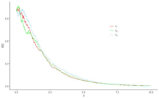
Figure 3. The simulated numbers of infected individuals under condition (a) of Theorem 2.

Example 2.

We set $T=10$and$\mathsf{\Delta }t=0.01$. Assume the parameters are given by$b=1, {\sigma }_k^2=0.4, k=1,2,3$,$\left({\beta }_{01},{\beta }_{02},{\beta }_{03}\right)=\left(0.6,0.5,0.4\right)$,$\left({\mu }_1,{\mu }_2,{\mu }_3\right)=\left(0.4,0.4,0.4\right)$,${\mu }_N=0.1$,$\left(q_0,q_1\right)=\left(0.8,0.6\right)$,$\left({\epsilon }_1,{\epsilon }_2\right)=\left(0.9,0.5\right)$, and$\delta =0.1$.

Then, we have ${max}_{k\in \left\{1,2,3\right\}}{R}_{0k}^S=0.2813<1$and${max}_{k\in \left\{1,2,3\right\}}\frac{{\beta }_{0k}^2}{2\left({\mu }_N+{\mu }_k+{\gamma }_k\right)}=0.12<0.4$,$k=1,2,3$. The model meets condition (b) of Theorem 2. As $S^0=1.8750$and${\beta }_{0k}<S^0{\sigma }_k^2$,$k=1,2,3$, it does not meet condition (a) of Theorem 2.

We simulated the numbers of infected individuals for each of three strains. The results are shown in Figure 4, indicating that the number of infected individuals approached 0 with time.

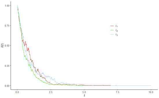
Figure 4. The simulated numbers of infected individuals under condition (b) of Theorem 2.

Example 3.

We set $T=300$and$\mathsf{\Delta }t=0.01$. Assume the parameters are given by$b=1, \left({\sigma }_1^2,{\sigma }_2^2,{\sigma }_3^2\right) =\left(0.0025,0.0020,0.0020\right)$,$\left({\beta }_{01},{\beta }_{02},{\beta }_{03}\right)=\left(0.28,0.20,0.24\right)$,$\left({\mu }_1,{\mu }_2,{\mu }_3\right)=\left(0.04,0.01,0.01\right)$,$\left({\gamma }_1,{\gamma }_2,{\gamma }_3\right)=\left(0.1,0.1,0.4\right),$ ${\mu }_N=0.1$,$\left(q_0,q_1\right)=\left(0.64,0.8\right)$, $\left({\epsilon }_1,{\epsilon }_2\right)=\left(0.3,0.1\right)$, and$\delta =0.1.$

Then, the basic reproduction numbers are$\left(R_{01},R_{02},R_{03}\right)=\left(3.1818,2.5974,1.2834\right)$,$\left(R_{01}^S,R_{02}^S,R_{03}^S\right)=\left(3.1430,2.5620,1.2688\right)$, and$\left(R_{01}^{*},R_{02}^{*},R_{03}^{*}\right)=\left(2.6610,2.1212,1.0873\right)$. We have${\overline{k}}^{*}=1$. As$S^0=2.7273$, it implies${\beta }_{0k}>S^0{\sigma }_k^2$,$k=1,2,3$.

We simulated the numbers of infected individuals of the three strains and we present the results in Figure 5.

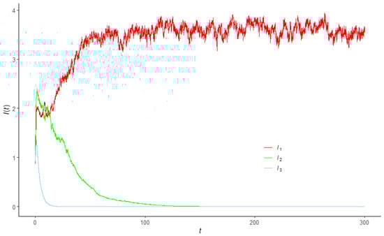
Figure 5. The simulated numbers of infected individuals under the conditions of the disease persistence.

Note that $\frac{{\sigma }_2^2{\beta }_{01}}{{\sigma }_1^2{\beta }_{02}}=1.1200>1$, $\frac{{\sigma }_1^2}{\left({\mu }_N+{\mu }_1+{\gamma }_1\right)}=0.0104>0.0095=\frac{{\sigma }_2^2}{\left({\mu }_N+{\mu }_2+{\gamma }_2\right)}$, $\frac{{\sigma }_3^2{\beta }_{01}}{{\sigma }_1^2{\beta }_{03}}=0.9333<1$, and $\frac{{\sigma }_3^2}{\left({\mu }_N+{\mu }_3+{\gamma }_3\right)}=0.0039>0.0013=\left(\frac{R_{03}^S-1}{R_{01}^S-1}\right)\frac{{\sigma }_1^2}{\left({\mu }_N+{\mu }_1+{\gamma }_1\right)}$. Obviously, only the first strain will persist, and the other two strains will go extinct.

Moreover, we assume cost model (31) with the costs $c_0=1.2$, $c_1=1$, and $C_0=4$. The optimal $q_1=0.8851$, and we have the optimal basic reproduction number $R_0^S=2.6804$. Note that if no one is vaccinated at all, $\underset{q_1\to 0}{\lim }{R}_0^s=11.1458$.

If we assume cost model (36) with $c_0=1.2$, $c_1=1$, and $c_2=5$, then the optimal $q_1=0.9044$ and we have $\overline{\xi }=3.8743$. If no one is vaccinated at all, $\underset{q_1\to 0}{\lim }\overline{\xi }=5.9681$.

Example 4.

We use the same setting for all parameters as that in Example 3 except for$T$and$\left(q_0,q_1\right)$. We set$T=100$and both$q_0$and$q_1$take 3 levels, 0.1, 0.5, and 0.9. The $R_0^S$’s and$\overline{\xi }$’srelated to different$\left(q_0,q_1\right)$combinations are shown inTable 3. All$R_0^S$’s and$\overline{\xi }$’s decrease as$q_0$and$q_1$increase. This echoes the sensitivity analysis in Section 2. It also means that the higher the vaccination rate, the higher the immune effect that can be achieved.

Table 3. The different $\left(q_0, q_1\right)$ combinations and related ${\mathit{R}}_0^{\mathit{S}}$’s and $\overline{\mathit{\xi }}$’s.

$\left({\mathit{q}}_0,{\mathit{q}}_1\right)$	${\mathit{R}}_0^{\mathit{S}}$	$\overline{\mathit{\xi }}$
(0.1, 0.1)	8.6662	5.7327
(0.1, 0.5)	8.1300	5.6695
(0.1, 0.9)	7.9410	5.6458
(0.5, 0.1)	4.5833	4.9769
(0.5, 0.5)	3.9022	4.7210
(0.5, 0.9)	3.6912	4.6240
(0.9, 0.1)	3.1151	4.2961
(0.9, 0.5)	2.5669	3.8537
(0.9, 0.9)	2.4041	3.6848

We simulated the total number of infected individuals by three strains (${\sum }_{k=1}^3{I}_k\left(t\right)$) and we present the results in Figure 6. The number of total infected individuals fluctuated within a fixed range after a certain time point. The level of its oscillation position is related to the vaccination rate.

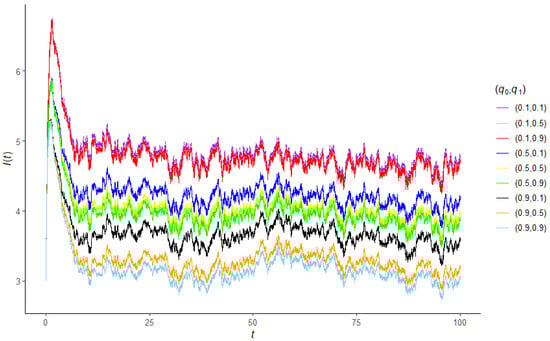
Figure 6. The simulated numbers of total infected individuals under the different $\left(q_0,q_1\right)$ combinations.

Example 5.

In order to mimic the actual COVID-19 infection situation, we consult the parameter information in Table 1 in [22] for simulation. First, we set b = 10 and μ_N = 0.01 to meet the value of$N^{*}$in the table, and we use the data in the table to set $\delta =\frac{1}{180}$,${\mu }_k=0.01\times \frac{1}{14}$, and${\gamma }_k=0.99\times \frac{1}{14}$,$k=1,2,3$. We assume that people who received one dose of the vaccine had twice the rate of loss of immunity compared with those who received two doses. Then, we set ${\epsilon }_2=\frac{1}{180}$and${\epsilon }_1=\frac{1}{90}$. As the vaccination rate is between 0.001 and 0.015, we set$\left(q_0,q_1\right)=\left(0.01, 0.015\right)$. As the transmission rate is between$\frac{0.055}{N}$and$\frac{0.18}{N}$in the table, we assign$\left({\beta }_1,{\beta }_2,{\beta }_3\right)=\frac{1}{1000}\times \left(0.18, 0.15,0.06\right)$and$\left({\sigma }_1,{\sigma }_2,{\sigma }_3\right)=\frac{1}{1000}\times \left(0.12, 0.10,0.04\right)$.

Then, the basic reproduction numbers are$\left(R_{01},R_{02},R_{03}\right)=\left(1.4317,1.1931,0.4772\right)$,$\left(R_{01}^S,R_{02}^S,R_{03}^S\right)=\left(1.3946,1.1673,0.4731\right)$, and$\left(R_{01}^{*},R_{02}^{*},R_{03}^{*}\right)=\left(1.3433,1.1317,0.4674\right)$.

We simulated the numbers of infected individuals of the three strains with $T=100$, and the initial conditions are given as $S\left(0\right)=967$, $R\left(0\right)=V_1\left(0\right)=V_2\left(0\right)=1$, and $I_k\left(0\right)=10$, $k=1,2,3$. The results are presented in Figure 7.

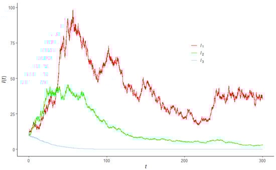
Figure 7. The simulated numbers of infected individuals under the conditions of Table 1 in [22].

As the $R_{01}^S$ and $R_{02}^S$ are both greater than 1, the number of infected patients gradually increases at the beginning and then decline after reaching a peak. The second strain slowly goes extinct, while the first strain continues oscillating between 25 and 50. $R_{03}^S$ is less than 1, and it tends to go extinct from the beginning. This phenomenon can reflect that changes in the epidemic often return to a relatively flat fluctuation after a wave of peaks.

5. Conclusions

In this study, we construct a stochastic multi-strain SIR model based on the current phenomenon of COVID-19 and consider the situation of two-dose vaccine administration. We use the basic reproduction number of this model, $R_0^S$, to establish the thresholds for disease extinction. In the discussions for persistence, we use another version of the basic reproduction number to find a lower bound on the number of infected patients. Although using the lower bound here may underestimate the number of infected patients, the result is mainly to guarantee the conditions for the persistent phenomenon. At the same time, we also point out the conditions under which some strains may go extinct in the competition of survival among multiple strains.

Finally, we introduce two cost models by leveraging the features of this model. That is, when minimizing the basic reproduction number or the number of infected individuals, we take the cost into consideration and provide the best two-dose vaccine administration rate. We also illustrate relevant theoretical results using numerical examples.

Our model has also a few limitations. The proposed model only considers the situation of one vaccine, and the failure mode of the vaccine is only expressed as the failure rate. Additionally, we do not discuss breakthrough infections and the potential for vaccines to reduce the disease severity and mortality. These are all directions that can be improved in the future.

References

- Kermack, W.O.; McKendrick, A.G. A contribution to the mathematical theory of epidemics. Proc. R. Soc. Lond. Ser. A Contain. Pap. A Math. Phys. Character 1927, 115, 700–721. [Google Scholar]
- Anderson, R.M.; May, R.M. Population biology of infectious diseases: Part I. Nature 1979, 280, 361–367. [Google Scholar] [CrossRef] [PubMed]
- May, R.M.; Anderson, R.M. Population biology of infectious diseases: Part II. Nature 1979, 280, 455–461. [Google Scholar] [CrossRef] [PubMed]
- Capasso, V.; Serio, G. A generalization of the Kermack-McKendrick deterministic epidemic model. Math. Biosci. 1978, 42, 43–61. [Google Scholar] [CrossRef]
- Martcheva, M. An Introduction to Mathematical Epidemiology; Springer: Boston, MA, USA, 2015. [Google Scholar]
- Gray, A.; Greenhalgh, D.; Hu, L.; Mao, X.; Pan, J. A stochastic differential equation SIS epidemic model. SIAM J. Appl. Math. 2011, 71, 876–902. [Google Scholar] [CrossRef] [Green Version]
- Méndez, V.; Campos, D.; Horsthemke, W. Stochastic fluctuations of the transmission rate in the susceptible-infected-susceptible epidemic model. Phys. Rev. E 2012, 86, 011919. [Google Scholar] [CrossRef] [Green Version]
- Cai, Y.; Kang, Y.; Banerjee, M.; Wang, A. A stochastic SIRS epidemic model with infectious force under intervention strategies. J. Differ. Equ. 2015, 259, 7463–7502. [Google Scholar] [CrossRef]
- Chen, C.; Kang, Y. Dynamics of a stochastic multi-strain SIS epidemic model driven by Levy noise. Commun. Nonlinear Sci. Numer. Simul. 2017, 43, 379–395. [Google Scholar] [CrossRef]
- Hethcote, H.; Ma, Z.; Liao, S. Effects of quarantine in six endemic models for infectious diseases. Math. Biosci. 2002, 180, 141–160. [Google Scholar] [CrossRef]
- Huang, S.; Chen, F.; Chen, L. Global dynamics of a network-based SIQRS epidemic model with demographics and vaccination. Commun. Nonlinear Sci. Numer. Simul. 2017, 43, 296–310. [Google Scholar] [CrossRef]
- Li, K.; Zhu, G.; Ma, Z.; Chen, L. Dynamic stability of an SIQS epidemic network and its optimal control. Commun. Nonlinear Sci. Numer. Simul. 2019, 66, 84–95. [Google Scholar] [CrossRef]
- Zhao, R.; Liu, Q.; Sun, M. Dynamical behavior of a stochastic SIQS epidemic model on scale-free networks. J. Appl. Math. Comput. 2022, 68, 813–838. [Google Scholar] [CrossRef]
- Zhang, X.B.; Zhang, X.H. The threshold of a deterministic and stochastic SIQS epidemic model with varying total population size. Appl. Math. Model. 2021, 91, 749–767. [Google Scholar] [CrossRef]
- Li, J.; Ma, Z. Qualitative analyses of SIS epidemic model with vaccination and varying total population size. Math. Comput. Model. 2002, 35, 1235–1243. [Google Scholar] [CrossRef]
- Li, J.; Ma, Z. Global analysis of SIS epidemic models with variable total population size. Math. Comput. Model. 2004, 39, 1231–1242. [Google Scholar]
- Zhao, Y.; Zhang, Q.; Jiang, D. The asymptotic behavior of a stochastic SIS epidemic model with vaccination. Adv. Differ. Equ. 2015, 2015, 328. [Google Scholar] [CrossRef] [Green Version]
- Zaman, G.; Kang, Y.H.; Jung, I.H. Stability analysis and optimal vaccination of an SIR epidemic model. Biosystems 2008, 93, 240–249. [Google Scholar] [CrossRef]
- Fudolig, M.; Howard, R. The local stability of a modified multi-strain sir model for emerging viral strains. PLoS ONE 2020, 15, e0243408. [Google Scholar] [CrossRef]
- World Health Organization. Coronavirus Disease (COVID-2019) Situation Reports. Available online: https://www.who.int/emergencies/diseases/novel-coronavirus-2019/situation-reports (accessed on 22 April 2022).
- Dong, Y.; Dai, T.; Wei, Y.; Zhang, L.; Zheng, M.; Zhou, F. A systematic review of SARS-CoV-2 vaccine candidates. Signal Transduct. Target. Ther. 2020, 5, 237. [Google Scholar] [CrossRef]
- Rella, S.A.; Kulikova, Y.A.; Dermitzakis, E.T.; Kondrashov, F.A. Rates of SARS-CoV-2 transmission and vaccination impact the fate of vaccine-resistant strains. Sci. Rep. 2021, 11, 15729. [Google Scholar] [CrossRef]
- Zheng, Q.; Wang, X.; Bao, C.; Ma, Z.; Pan, Q. Mathematical modelling and projecting the second wave of COVID-19 pandemic in Europe. J. Epidemiol. Community Health 2021, 75, 601–603. [Google Scholar] [CrossRef] [PubMed]
- Zheng, Q.; Wang, X.; Bao, C.; Ji, Y.; Liu, H.; Meng, Q.; Pan, Q. A multi-regional hierarchical-tier mathematical model of the spread and control of COVID-19 epidemics from epicentre to adjacent regions. Transbound. Emerg. Dis. 2022, 69, 549–558. [Google Scholar] [CrossRef] [PubMed]
- Zheng, Q.; Wang, X.; Pan, Q.; Wang, L. Optimal strategy for a dose-escalation vaccination against COVID-19 in refugee camps. AIMS Math. 2022, 7, 9288–9310. [Google Scholar] [CrossRef]
- Blower, S.M.; Dowlatabadi, H. Sensitivity and uncertainty analysis of complex models of disease transmission: An HIV model, as an example. Int. Stat. Rev. 1994, 62, 229–243. [Google Scholar] [CrossRef]
- Zhang, K.; Wang, X.; Liu, H.; Ji, Y.; Pan, Q.; Wei, Y.; Ma, M. Mathematical analysis of a human papillomavirus transmission model with vaccination and screening. AIMS Math. Biosci. Eng. 2020, 17, 5449–5476. [Google Scholar] [CrossRef]
- Husnulkhotimah, H.; Rusin, R.; Aldila, D. Using the SVIRS model to understand the prevention strategy for influenza with vaccination. AIP Conf. Proc. 2021, 2374, 030004. [Google Scholar]
- Mao, X. Stochastic Differential Equations and Applications; Horwood Publishing: Chichester, UK, 1997; pp. 12–13. [Google Scholar]
Publisher’s Note: MDPI stays neutral with regard to jurisdictional claims in published maps and institutional affiliations. |
© 2022 by the authors. Licensee MDPI, Basel, Switzerland. This article is an open access article distributed under the terms and conditions of the Creative Commons Attribution (CC BY) license (https://creativecommons.org/licenses/by/4.0/).