Domination and Independent Domination in Hexagonal Systems

Abstract

A vertex subset D of G is a dominating set if every vertex in $V\left(G\right)\backslash D$ is adjacent to a vertex in D. A dominating set D is independent if $G\left[D\right]$, the subgraph of G induced by D, contains no edge. The domination number $\gamma \left(G\right)$ of a graph G is the minimum cardinality of a dominating set of G, and the independent domination number $i\left(G\right)$ of G is the minimum cardinality of an independent dominating set of G. A classical work related to the relationship between $\gamma \left(G\right)$ and $i\left(G\right)$ of a graph G was established in 1978 by Allan and Laskar. They proved that every $K_{1,3}$-free graph G satisfies $\gamma \left(G\right)=i\left(H\right)$. Hexagonal systems (2 connected planar graphs whose interior faces are all hexagons) have been extensively studied as they are used to present bezenoid hydrocarbon structures which play an important role in organic chemistry. The domination numbers of hexagonal systems have been studied continuously since 2018 when Hutchinson et al. posted conjectures, generated from a computer program called Conjecturing, related to the domination numbers of hexagonal systems. Very recently in 2021, Bermudo et al. answered all of these conjectures. In this paper, we extend these studies by considering the relationship between the domination number and the independent domination number of hexagonal systems. Although every hexagonal system H with at least two hexagons contains $K_{1,3}$ as an induced subgraph, we find many classes of hexagonal systems whose domination number is equal to an independent domination number. However, we establish the existence of a hexagonal system H such that $\gamma \left(H\right)<i\left(H\right)$ with the prescribed number of hexagons.

1. Motivation

Let $G=\left(V\right(G),E(G\left)\right)$ be a graph with the vertex set $V\left(G\right)$ and edge set $E\left(G\right)$. For two vertices $u,v\in V\left(G\right)$, the distance between u and v is the length of a shortest path from u to v. The open neighborhood $N\left(v\right)$ of a vertex v in G is the set $\{u\in V(G)\mid uv\in E(G\left)\right\}$. The degree of a vertex v is $\left|N\right(v\left)\right|$. A star $K_{1,k}$ is obtained from $k+1$ vertices by joining one vertex to all the other k vertices. For a set $A\subseteq V\left(G\right)$, the subgraph of G induced by A is denoted by $G\left[A\right]$. For a family $\mathcal{F}$ of graphs, a graph G is $\mathcal{F}$-free if G does not contain F as an induced subgraph for any $F\in \mathcal{F}$.

A set $D\subseteq V\left(G\right)$ is a dominating set of a graph G if every vertex v in $V\left(G\right)\backslash D$ is adjacent to a vertex in D. The domination number of G is the minimum cardinality of a dominating set of G and is denoted by $\gamma \left(G\right)$. If D is a dominating set of G, then we write $D\succ G$. A dominating set I is independent if $G\left[I\right]$ contains no edge. The independent domination number of G is the minimum cardinality of an independent dominating set of G and is denoted by $i\left(G\right)$. A set $D\subseteq V\left(G\right)$ is packing of G if $N\left[u\right]\cap N\left[v\right]=\varnothing$ for any two distinct vertices $u,v\in D$. The packing number of G is the maximum cardinality of a packing in G and is denoted by $\rho \left(G\right)$. Furthermore, a set $D\subseteq V\left(G\right)$ is a packing-independent dominating set of G if D is both the packing and independent dominating set of G. It is well-known that for any graph G:

$$\begin{array}{c}\hfill \rho \left(G\right)\le \gamma \left(G\right)\le i\left(G\right).\end{array}$$

Thus, if D is a packing-independent dominating set of G, then $\left|D\right|=\rho \left(G\right)=i\left(G\right)$. As $\rho \left(G\right)$ is not always equal to $i\left(G\right)$ for any graph G, the packing-independent dominating set of G does not always exist either. However, if G has a packing-independent dominating set, then:

$$\begin{array}{c}\hfill \rho \left(G\right)=\gamma \left(G\right)=i\left(G\right).\end{array}$$

A hexagonal system H is a finite 2-connected plane graph whose interior faces of H are all mutually congruent regular hexagons. Two hexagons (faces) of H are adjacent if they share a common edge. Hence, the exterior face of H is its perimeter which consists of sides of hexagons that are not sharing. Observe that every vertex of H has a degree of 2 or 3. An internal vertex of H is a vertex which does not lie on the exterior face. In Figure 1, the hexagon $h_1$ is adjacent to the hexagon $h_2$, but $h_1$ is not adjacent to the hexagon $h_3$. Furthermore, $x_1$ and $x_2$ are the only two internal vertices of this hexagonal system. As we know that every edge of a graph always has two end vertices, to simplify all our figures from now, we may draw all the figures with edges (line segments) only. Two edges are incidents of the two corresponding line segments’ ends at the same corner of a hexagon. All the circular vertices in our figures are used to present the vertices in a dominating set or a packing instead.

Figure 1. An example of a hexagonal system.

A hexagonal system is catacondensed if it does not possess any internal vertex, otherwise, the hexagonal system is called pericondensed. Thus, every hexagon of a catacondensed hexagonal system is adjacent to at most three hexagons while every hexagon of a pericondensed hexagonal system is adjacent to at most six hexagons. A hexagon h of a catacondensed hexagonal system is branching if h is adjacent to three hexagons. More examples of catacondensed and pericondensed hexagonal systems are given in Section 2.

Over the past few decades, benzenoid hydrocarbon C${}_{\mathrm{k}}$H${}_{\mathrm{l}}$ have caught attentions of both experimental and theoretical chemists as it has large scale in industrial applications. This is the reason why structural properties of benzenoid species have been extensively investigated. Interestingly, all structures of bezenoid hydrocarbons can be illustrated by graphs. We ignore hydrogen atoms while each carbon atom is corresponding to a vertex. Two vertices are adjacent if the two atoms are bonded. Since all fused rings of bezenoid hydrocarbon are hexagon-like shapes, all the structures of these compounds are presented by hexagonal systems. The domination numbers of hexagonal systems have been studied continuously since 2018 when Hutchinson et al. [1] developed computer program called Conjecturing from Fajtlowics’s dalmation heuristic to generate conjectures related to the domination numbers of hexagonal systems. The authors in [1] have finished proving some of their own conjectures obtaining from the program and posted some that they could not. Very recently in 2021, Bermudo et al. [2] answered all of these conjectures. Bermudo et al. [2,3] further proved some more results related with domination numbers of hexagonal systems as detailed in the following theorems:

Theorem 1

([2]). Let H be a catacondensed hexagonal system containing n hexagons, $a_3$ of which are branching. If any two branching hexagons of H are not adjacent, then:

$$n+1+\lceil \frac{a_3}{2}\rceil \le \gamma \left(H\right).$$

Proposition 1

([3]). If H is a zigzag hexagonal system (the definition of this graph will be given in Section 2) containing n hexagons, then:

$$\gamma \left(H\right)=n+\lfloor \frac{n+1}{5}\rfloor +1.$$

For more works in the literature that investigate the domination numbers of chemical graphs, see [4,5] for example. For a paper that investigated the connection between the domination number and RNA structures, see [6].

The study of domination and independent domination numbers of a graph was started in 1978 by Allan and Laskar [7], which found the equality of these parameters when the graphs do not contain $K_{1,3}$ as an induced subgraph. This motivated Topp and Volkmann [8] to characterize the family $\mathcal{F}$ of 16 forbidden graphs for a graph G to satisfy the equation $\gamma \left(G\right)=i\left(G\right)$, one of which is illustrated by Figure 2.

Figure 2. The graph $F_1$.

That is, Topp and Volkmann [8] proved the following:

Theorem 2.

If a graph G is $\mathcal{F}$-free, then $\gamma \left(G\right)=i\left(G\right)$.

Clearly, every hexagonal system H that has more than one hexagon contains $K_{1,3}$ and $F_1$ as induced subgraphs. Hence, by the results from Allan and Laskar [7] and from Topp and Volkmann [8] in Theorem 2, we have that $i\left(H\right)$ and $\gamma \left(G\right)$ need not be the same value. Thus, the question that is arisen is:

Question 1.

Which classes of hexagonal systems H satisfy $\gamma \left(H\right)=i\left(H\right)$?

In this paper, in spite of all hexagonal systems having at least two hexagons contain $K_{1,3}$ and $F_1$ as induced subgraphs, we show that there are many classes of hexagonal systems whose domination number is equal to the independent domination number. However, we prove that for any $n\ge 8$, there exists a hexagonal system H with n hexagons such that $\gamma \left(H\right)<i\left(H\right)$. For more studies on domination and independent domination numbers of a graph, see [9,10,11] for example.

This paper is organized as follows. In Section 2, we provide definitions of many classes of catacondensed and pericondensed hexagonal systems, which we will establish domination and independent domination numbers of these graphs. In Section 3, we state all the main results in this paper, where the proofs are given in Section 4. We finish this paper with some conjectures in Section 5.

2. Catacondensed and Pericondensed Hexagonal Systems

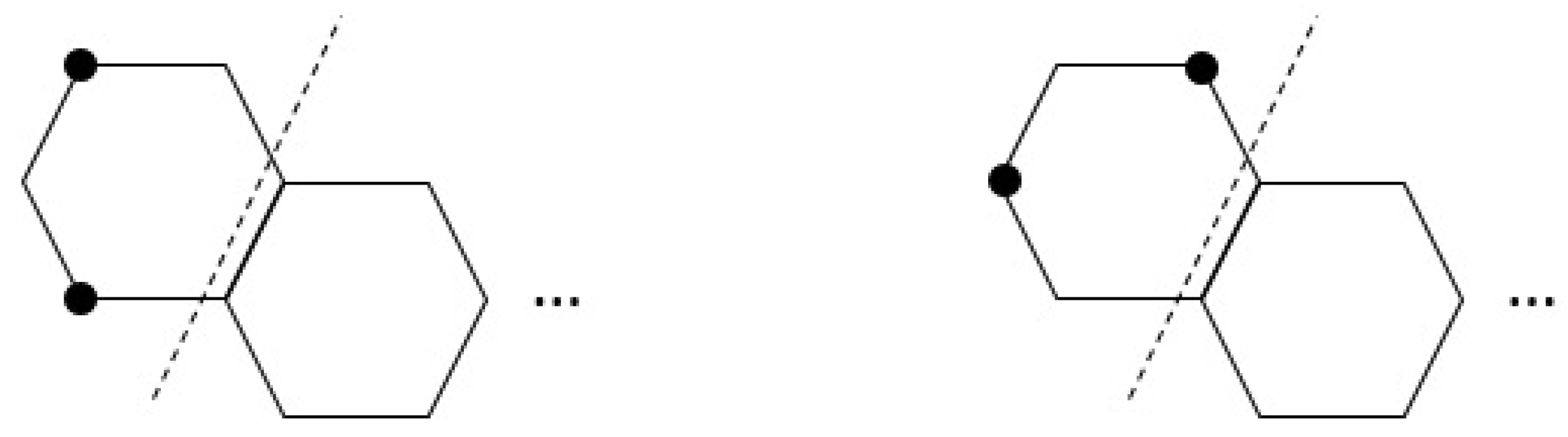
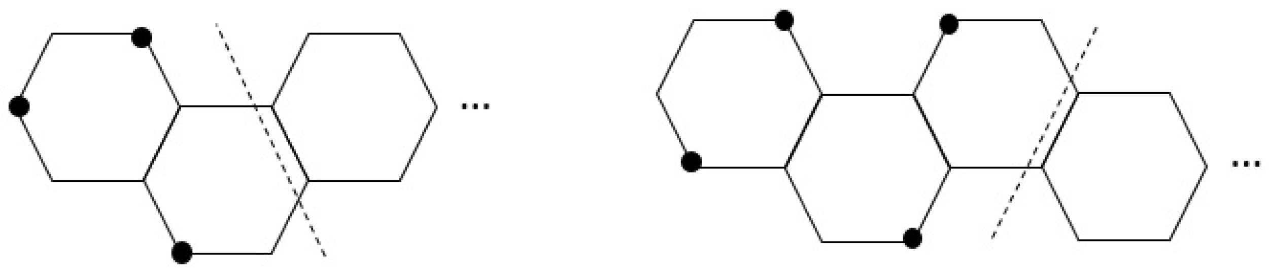
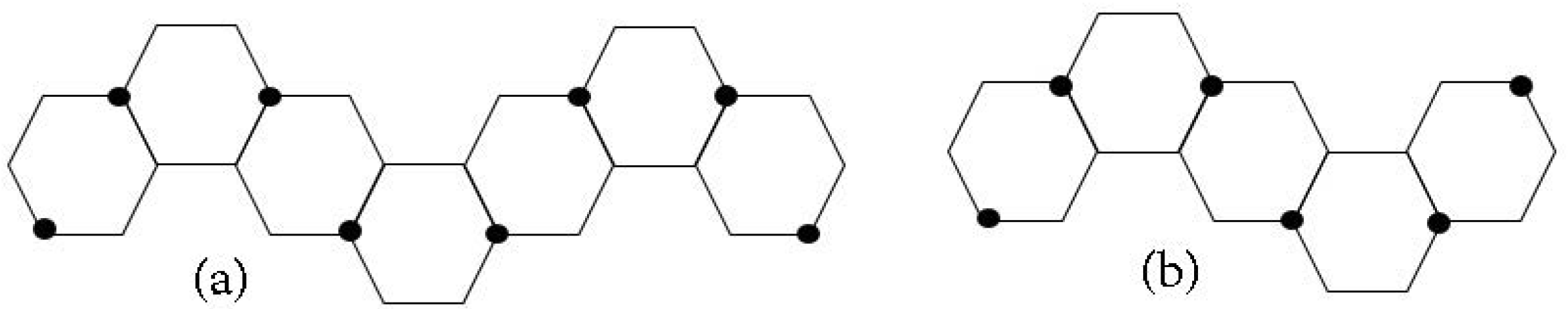
2.1. Catacondensed Hexagonal Systems

In a catacondensed hexagonal system H, if a hexagon h is adjacent to three hexagons, then h is called a branching hexagon of H. The number of branching hexagons of H is denoted by $a_3$. An edge e is $e_{2,2}$ if both end vertices of e have a degree of two. The dual tree $DT\left(H\right)$ of H is the tree whose vertices are the hexagons of H and two vertices $h,h^{\prime }$ of $DT\left(H\right)$ are adjacent if and only if the two corresponding hexagons $h,h^{\prime }$ of H are adjacent. Furthermore, H is said to be a chain if it has no branching hexagon (every hexagon is adjacent to at most two hexagons). A hexagon h is a leaf if h is adjacent to exactly one hexagon. In Figure 3, a catacondensed hexagonal system H has $h_1$ as a leaf and has $h_2$ as a branching hexagon. The dual tree $DT\left(H\right)$ is illustrated on the right.

Figure 3. A catacondensed hexagonal system H and its dual $DT\left(H\right)$.

Clearly, a hexagonal chain has exactly two leaves. Thus, in a hexagonal chain containing n hexagons $h_1,\dots ,h_n$, renaming all the hexagons if necessary, we may let $h_1$ and $h_n$ be the two leaves while the hexagon $h_i$ is adjacent to the hexagons $h_{i-1}$ and $h_{i+1}$ for $2\le i\le n-1$. Since a hexagonal chain C has no branching hexagon, its dual tree becomes the dual path $DP\left(C\right)$, whose vertices are $h_1,\dots ,h_n$ such that $h_1,h_n$ are the two vertices of degree one while the vertex $h_i$ is adjacent to only the vertices $h_{i-1}$ and $h_{i+1}$ for $2\le i\le n-1$. Note that we may construct the dual path $DP\left(C\right)$ by adding a vertex $h_i$ to the middle of hexagon $h_i$ of C. Then, we join vertices $h_i,h_{i+1}$ by drawing an edge (of the path) crossing the common edge of hexagons $h_i,h_{i+1}$. The following definitions are defined when we move along the dual path from $h_1$ to $h_n$. A hexagon h is linear (L) if (i) h is either $h_1$ or $h_n$ or (ii) the two vertices of degree two of h are on the different sides of the dual path $DP\left(C\right)$. A hexagon h is left angular ($LA$) if the two vertices of degree two of h are both on the right hand side of $DP\left(C\right)$ while h is right angular ($RA$) if the two vertices of degree two of h are both on the left hand side of $DP\left(C\right)$. Therefore, every hexagonal chain can be encoded by a sequence of $L,LA$ and $RA$. Figure 4 illustrates a hexagonal chain $C=L-LA-RA-LA-RA-L$.

Figure 4. The dual path (left) and the code (right) of a hexagonal chain C.

A hexagonal chain C is linear if all hexagons of C are linear. That is $C=L-L-\cdots -L$. A hexagonal chain C is zigzag if $C=L-LA-RA-LA-RA-\cdots -L$ or $C=L-RA-LA-RA-LA\cdots -L$. A hexagonal chain C is relaxed zigzag if $C=L-LA-L-RA-L-\cdots -LA-L-RA-L$ or $C=L-LA-L-RA-L-\cdots -RA-L-LA-L$. Figure 5 illustrates a zigzag $L-RA-LA-RA-LA-L$ (top left), a zigzag $L-RA-LA-RA-L$ (top right), a relaxed zigzag $L-RA-L-LA-L-RA-L$ (bottom left), and a relaxed zigzag $L-RA-L-LA-L$ (bottom right). For a catacondensed hexagonal system H having a leaf h, the graph $H\ominus h$ is obtained by removing all four vertices of degree two of h and all edges that are incident to each of these vertices from H. If $h^{\prime }$ is the hexagon of H that is adjacent to a leaf h, we simply write $H\ominus h\ominus h^{\prime }$ rather than $(H\ominus h)\ominus h^{\prime }$.

Figure 5. Examples of zigzag and relaxed zigzag hexagonal systems.

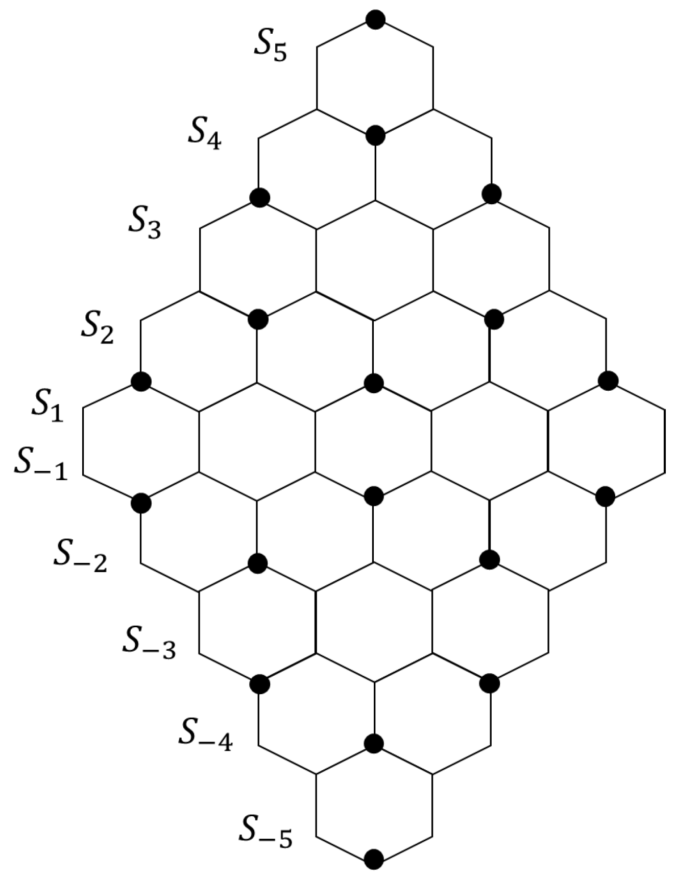
2.2. Pericondensed Hexagonal Systems

For pericondensed hexagonal systems, we focus on the following well-known classes. The first class of pericondensed hexagonal systems was introduced by Klobučar and Klobučar [12].

Hexagonal Grid $H_{n,m}$

We let $H_{n,m}$ be a hexagonal grid such that there are n hexagons in a row and there are m hexagons in a column. For $1\le i\le \lfloor \frac{m}{2}\rfloor$, the first hexagon of Row $2i$ share edges with the first and the second hexagons of Row $2i-1$. It can be observed that $H_{n,m}$ consists of $m+1$ horizontal zigzag paths, which we may call $P_1,\dots ,P_{m+1}$ from the bottom to the top of $H_{n,m}$, respectively. When $i\in \{1,m+1\}$, we may label all the vertices of $P_i$ as $v_{i,1},v_{i,2},\dots ,v_{i,2n+1}$ from the left to right of $H_{n,m}$, respectively. When $i\in \{2,\dots ,m\}$, we may label all the vertices of $P_i$ as $v_{i,1},v_{i,2},\dots ,v_{i,2n+2}$ from the left to right of $H_{n,m}$, respectively. It can be observed that, if $n=1$, then $H_{1,m}$ is a zigzag hexagonal chain while $H_{n,1}$ is a linear hexagonal chain. Figure 6 illustrates $H_{6,4}$.

Figure 6. The hexagonal grid $H_{6,4}$.

The next class of pericondensed hexagonal systems was introduced in the classical book of Gutman and Cyvin [13].

Prolate Rectangle $R_{n,m}$

We let $R_{n,m}$ be a prolate rectangle having $2m-1$ rows such that there are n hexagons in Row $2i-1$ and there are $n-1$ hexagons in Row $2i$ for $1\le i\le m$. The first hexagon of Row $2i$ shares edges with the first and the second hexagons of Row $2i-1$. It is worth noting that $R_{n,m}$ has m rows of n hexagons and $m-1$ rows of $n-1$ hexagons. It can be observed that $R_{n,m}$ consists of $2m$ horizontal zigzag paths, which we may call $P_1,\dots ,P_{2m}$ from the bottom to the top of $R_{n,m}$, respectively. For $1\le i\le 2m$, we may label all the vertices of $P_i$ as $v_{i,1},v_{i,2},\dots ,v_{i,2n+1}$. Figure 7 illustrates $R_{4,3}$.

Figure 7. The prolate rectangle $R_{4,3}$.

The last class of pericondensed hexagonal systems that we focus on in this paper was introduced by Quadras et al. [14].

Pyrene $P{R}_n$

For a natural number n, a pyrene $P{R}_n$ of dimension n consists of $2n-1$ rows of linear hexagonal systems $L_0,L_1,\dots ,L_{n-1},L_{-1},\dots ,L_{-(n-1)}$ such that $L_0$ contains n hexagons and, for every $1\le i\le n-1$, each of $L_i$ and $L_{-i}$ contains $n-i$ hexagons. Moreover, the first hexagon of $L_i$ shares one edge with the first hexagon of $L_{i-1}$ and shares one edge with the second hexagon of $L_{i-1}$. Similarly, the first hexagon of $L_{-i}$ shares one edge with the first hexagon of $L_{-(i-1)}$ and shares one edge with the second hexagon of $L_{-(i-1)}$. Examples of the pyrenes of dimensions 4 and 5 are illustrated in Figure 8. It is worth noting that, when $n=1$, a pyrene of dimension 1 is a hexagonal system containing exactly one hexagon. We may name vertices of $P{R}_n$ as follows. When $i>0$, the lower horizontal zigzag path of $L_i$ is $v_{i,1},v_{i,2},\dots ,v_{i,2(n-i)+3}$. When $i<0$, the upper horizontal zigzag path of $L_{-i}$ is $v_{-i,1},v_{-i,2},\dots ,v_{-i,2(n-i)+3}$.

Figure 8. Pyrenes $P{R}_4$ and $P{R}_5$.

3. Main Results

In this section, we state all the main results of this paper, while the proofs are given in Section 4. Our main results in the first subsection relate to the domination numbers and the independent domination numbers of pericondensed hexagonal systems while those for catacondensed hexagonal systems are stated in the second subsection.

3.1. Pericondensed Hexagonal Systems

Theorem 3.

For a hexagonal grid $H_{n,m}$ with n hexagons in a row and m hexagons $(m\ge 3)$ in a column, it holds that:

$$i\left(H_{n,m}\right)\le \left\{\begin{array}{cc}\frac{1}{2}m(n+1)+\lceil \frac{m-2}{4}\rceil +\lceil \frac{2n+1}{3}\rceil +2,\hfill & \mathit{if}n\mathit{and}m\mathit{are}\mathit{even}\hfill \\ \lceil \frac{n}{2}\rceil m+\lceil \frac{m-2}{4}\rceil +\lceil \frac{2n+1}{3}\rceil +1,\hfill & \mathit{if}n\mathit{is}\mathit{odd}\mathit{and}m\mathit{is}\mathit{even}\hfill \\ \lceil \frac{m}{2}\rceil (n+1)+\lceil \frac{m-2}{4}\rceil +1,\hfill & \mathit{if}n\mathit{is}\mathit{even}\mathit{and}m\mathit{is}\mathit{odd}\hfill \\ 2\lceil \frac{n}{2}\rceil \lceil \frac{m}{2}\rceil +\lceil \frac{m-2}{4}\rceil ,\hfill & \mathit{if}n\mathrm{and}m\mathit{are}\mathit{odd}.\hfill \end{array}\right.$$

Furthermore, it holds that:

$$\rho \left(H_{n,m}\right)\ge \left\{\begin{array}{cc}\frac{1}{2}m(n+1)+\lceil \frac{m-2}{4}\rceil +\lfloor \frac{n}{3}\rfloor ,\hfill & \mathit{if}n\mathit{and}m\mathit{are}\mathit{even}\hfill \\ \lceil \frac{n}{2}\rceil m+\lfloor \frac{n}{3}\rfloor ,\hfill & \mathit{if}n\mathit{is}\mathit{odd}\mathit{and}m\mathit{is}\mathit{even}\hfill \\ \lceil \frac{m}{2}\rceil (n+1),\hfill & \mathit{if}n\mathit{is}\mathit{even}\mathit{and}m\mathit{is}\mathit{odd}\hfill \\ 2\lceil \frac{n}{2}\rceil \lceil \frac{m}{2}\rceil ,\hfill & \mathit{if}n\mathit{and}m\mathit{are}\mathit{odd}.\hfill \end{array}\right.$$

Theorem 4.

For natural numbers $n,m$, a prolate rectangle $R_{n,m}$ satisfies

$$\rho \left(R_{n,m}\right)=\gamma \left(R_{n,m}\right)=i\left(R_{n,m}\right)=(n+1)⌈\frac{2m-1}{2}⌉.$$

Theorem 5.

For natural numbers $n\ge 1$, a pyrene $P{R}_n$ satisfies:

$$\rho \left(P{R}_n\right)=\gamma \left(P{R}_n\right)=i\left(P{R}_n\right)=\left\{\begin{array}{cc}{\left(\frac{n}{2}\right)}^2+{\left(\frac{n+2}{2}\right)}^2,\hfill & \mathit{if}n\mathit{is}\mathit{even}\hfill \\ {\left(\frac{n+1}{2}\right)}^2,\hfill & \mathit{if}n\mathit{is}\mathit{odd}.\hfill \end{array}\right.$$

3.2. Catacondensed Hexagonal Systems

Theorem 6.

If H is a catacondensed hexagonal system containing n hexagons, then the following assertions hold:

(a) 

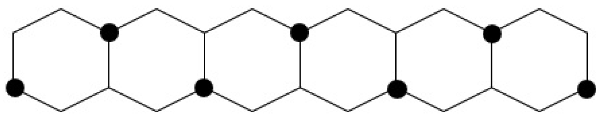
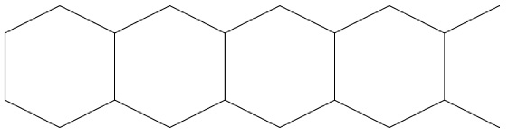
If H is a linear hexagonal chain, then $\rho \left(H\right)=\gamma \left(H\right)=i\left(H\right)=n+1$.

(b) 

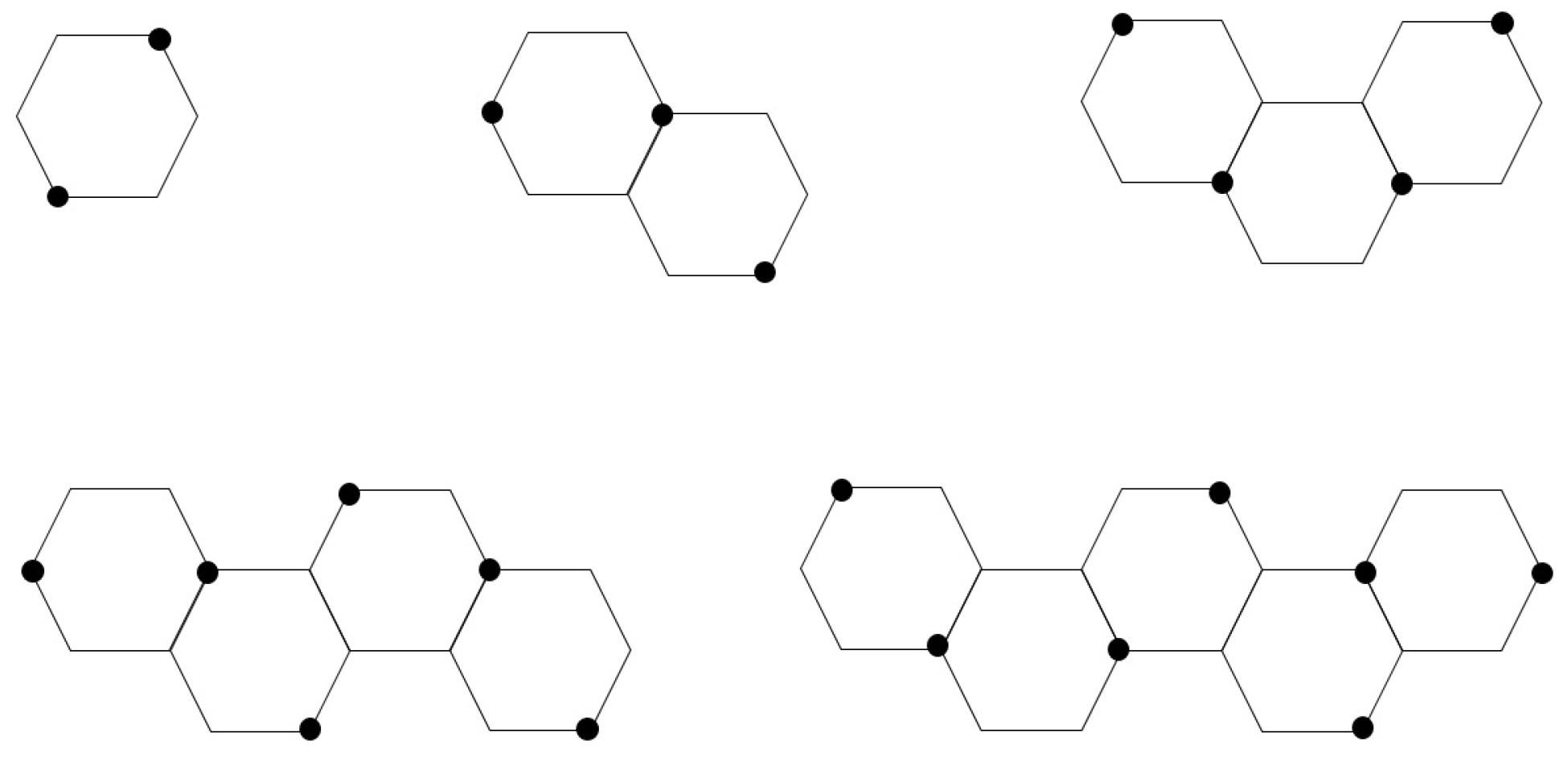
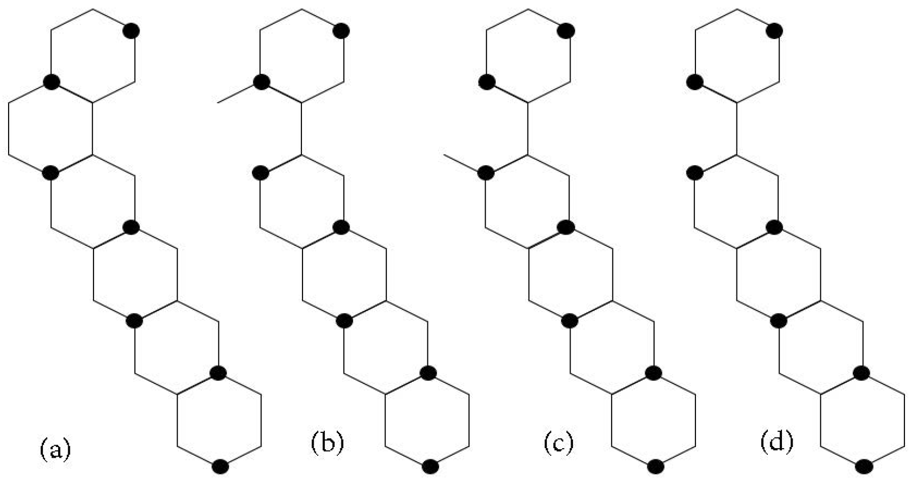
If H is a zigzag, then $\gamma \left(H\right)=i\left(H\right)=n+\lfloor \frac{n+1}{5}\rfloor +1$.

(c) 

If H is a relaxed zigzag, then $\rho \left(H\right)=\gamma \left(H\right)=i\left(H\right)=n+1$.

From most of the above main results, it seems there are not many hexagonal systems whose domination number is less than independent domination number. However, we establish the existence of a hexagonal system H with n hexagons such that $\gamma \left(H\right)<i\left(H\right)$ for any $n\ge 8$.

Let:

$\mathcal{CH}\left(n\right)$: the class of catacondensed hexagonal systems H such that $\gamma \left(H\right)<i\left(H\right)$.

Theorem 7.

For any $n\ge 8$, $\mathcal{CH}\left(n\right)\ne \varnothing$. That is, for any $n\ge 8$, there exists a catacondensed hexagonal system H containing n hexagons such that $\gamma \left(H\right)<i\left(H\right)$.

4. Proofs

4.1. Proof of Theorem 3

Proof. 

We will consider the number of cases according to m and n as odd or even and to m modulo 4 and n modulo 3, where $m\equiv kmod4$, $k=0,1,2,3$ and $n\equiv tmod3$, $t=0,1,2$.

Case 1.n and m are even.

Case 1.1.$k=0$ and $t=0,2$.

We let:

$L_{4i+2}=\{v_{4i+2,4j+1}:j\in \{0,1,2,\dots ,\frac{n}{2}\}\}$ for all $i\in \{0,1,2,3,\dots ,\frac{m}{4}-1\}$;

$L_{4i+3}=\{v_{4i+3,4j+3}:j\in \{0,1,2,\dots ,\frac{n}{2}-1\}\}$ for all $i\in \{0,1,2,3,\dots ,\frac{m}{4}-1\}$;

$L_{4i}=\{v_{4i,4j+3}:j\in \{0,1,2,\dots ,\frac{n}{2}-1\}\}$ for all $i\in \{1,2,3,\dots ,\frac{m}{4}\}$;

$L_{4i+1}=\{v_{4i+1,4j+1}:j\in \{0,1,2,\dots ,\frac{n}{2}\}\}$ for all $i\in \{1,2,3,\dots ,\frac{m}{4}\}$.

Note that $|L_2\cup L_3\cup \cdots \cup L_{m+1}|=2\lceil \frac{n}{2}\rceil \lceil \frac{m}{2}\rceil +\frac{m}{2}=\frac{1}{2}mn+\frac{m}{2}$, and these vertices dominate all vertices in $H_{n,m}$, except some vertices in $P_1$, the first zigzag path, and some vertices in the nth column.

Next, we let:

$L_1=\{v_{1,3i+1}:i\in \{0,1,2,3,...,\lceil \frac{2n+1}{3}\rceil -1\}\}.$

Thus, $|L_1|=\lceil \frac{2n+1}{3}\rceil$ and $L_1$ dominates all vertices in $P_1$.

We need to define a set $B_i$ of one vertex to dominate the rest of vertices in the last column. Let $B_i=\left\{v_{i+2,2n+2}\right\}$, where $i\in I=\{k+2,k+6,k+10,k+14,\dots ,m-2\}$. It is clear that $\left|I\right|=\lceil \frac{m-2}{4}\rceil$, so we need $\lceil \frac{m-2}{4}\rceil$ vertices to dominate the last nth column. See Figure 9 for an example of $H_{6,8}$. It can be checked that $\left({\bigcup }_{i=1}^{m+1}{L}_i\right)\cup \left({\bigcup }_{i\in I}{B}_i\right)$ is an independent dominating set of $H_{n,m}$. Because $|\left({\bigcup }_{i=1}^{m+1}{L}_i\right)\cup \left({\bigcup }_{i\in I}{B}_i\right)|=\frac{1}{2}nm+\frac{m}{2}+\lceil \frac{m-2}{4}\rceil +\lceil \frac{2n+1}{3}\rceil$, by the minimality of $i\left(H_{n,m}\right)$:

$$i\left(H_{n,m}\right)\le \frac{1}{2}m(n+1)+\lceil \frac{m-2}{4}\rceil +\lceil \frac{2n+1}{3}\rceil .$$

Figure 9. The hexagonal grid $H_{6,8}$ black vertices belong to $L_i$, and white vertices belong to $B_i$.

Case 1.2.$k=0$ and $t=1$.

Note that, in this case, the vertex $v_{1,2n+1}$ is not dominated, so we need to add it to $L_1$. Therefore:

$$i\left(H_{n,m}\right)\le \frac{1}{2}m(n+1)+\lceil \frac{m-2}{4}\rceil +\lceil \frac{2n+1}{3}\rceil +1.$$

Case 1.3.$k=2$ and $t=0$.

In this case, we let:

$L_{4i+2}=\{v_{4i+2,4j+3}:j\in \{0,1,2,\dots ,\frac{n}{2}-1\}\}$ for all $i\in \{0,1,2,3,\dots ,\frac{1}{4}(m-2)\}$;

$L_{4i+3}=\{v_{4i+3,4j+1}:j\in \{0,1,2,\dots ,\frac{n}{2}\}\}$ for all $i\in \{0,1,2,3,\dots ,\frac{1}{4}(m-2)\}$;

$L_{4i}=\{v_{4i,4j+1}:j\in \{0,1,2,\dots ,\frac{n}{2}\}\}$ for all $i\in \{1,2,3,\dots ,\frac{1}{4}(m-2)\}$;

$L_{4i+1}=\{v_{4i+1,4j+3}:j\in \{0,1,2,\dots ,\frac{n}{2}-1\}\}$ for all $i\in \{1,2,3,\dots ,\frac{1}{4}(m-2)\}$.

Note that $|L_2\cup L_3\cup \cdots \cup L_{m+1}|=\frac{1}{2}mn+\frac{m}{2}$. Furthermore, $L_1$ is defined the same as in Case $1.1$. We only need to add the vertex $v_{3,2n+1}$. Therefore:

$$i\left(H_{n,m}\right)\le \frac{1}{2}m(n+1)+\lceil \frac{m-2}{4}\rceil +\lceil \frac{2n+1}{3}\rceil +1.$$

Case 1.4.$k=2$ and $t=1$.

This case is the same as in Case $1.3$, the vertices $v_{1,2n+1}$ and $v_{3,2n+1}$ are added. Thus:

$$i\left(H_{n,m}\right)\le \frac{1}{2}m(n+1)+\lceil \frac{m-2}{4}\rceil +\lceil \frac{2n+1}{3}\rceil +2.$$

Case 1.5.$k=2$ and $t=2$.

This case is the same as in Case $1.3$. We only need to add the vertex $v_{2,2n+2}$. Therefore:

$$i\left(H_{n,m}\right)\le \frac{1}{2}m(n+1)+\lceil \frac{m-2}{4}\rceil +\lceil \frac{2n+1}{3}\rceil +2.$$

Now, we will consider the packing number if n and m are even. Note that all vertices that belong to $L_2,L_3,L_4,\dots ,L_{m+1}$ in all sub-cases are packing. Let $L_1^{\ast }=\{v_{1,6i+4},i=0,1,2,\dots ,\lfloor \frac{n}{3}\rfloor -1\}$. Thus, $|L_1^{\ast }|=\lfloor \frac{n}{3}\rfloor$. All vertices in $L_1^{\ast }$ are packing. Hence:

$$\rho \left(H_{n,m}\right)\ge \frac{1}{2}m(n+1)+\lceil \frac{m-2}{4}\rceil +\lfloor \frac{n}{3}\rfloor .$$

Case 2.n is odd and m is even.

Case 2.1.$k=0$ and $t=1,2$.

Let $L_1,L_2,L_4,\dots ,L_{m+1}$ be defined the same as in Case 1.1. In addition, we need to define a set $B_i$ of one vertex to dominate the vertices in the last column, as in Case 1.1. See Figure 10 for an example of $H_{9,10}$. So, we need $\lceil \frac{m-2}{4}\rceil$ vertices. Therefore:

$$i\left(H_{n,m}\right)\le m\lceil \frac{n}{2}\rceil +\lceil \frac{m-2}{4}\rceil +\lceil \frac{2n+1}{3}\rceil .$$

Figure 10. The hexagonal grid $H_{9,10}$.

Case 2.2.$k=0$ and $t=0$.

This case is the same as Case $2.1$, except we need to remove the vertex $v_{2,2n+2}$. Hence:

$$i\left(H_{n,m}\right)\le m\lceil \frac{n}{2}\rceil +\lceil \frac{m-2}{4}\rceil +\lceil \frac{2n+1}{3}\rceil -1.$$

Case 2.3.$k=2$ and $t=0,2$.

We let $L_1,L_2,L_3,\dots ,L_{m+1}$ be the same as in Case 1.3, and we define B the same as in Case 2.1. Hence:

$$i\left(H_{n,m}\right)\le m\lceil \frac{n}{2}\rceil +\lceil \frac{m-2}{4}\rceil +\lceil \frac{2n+1}{3}\rceil .$$

Case 2.4. if $k=2$ and $t=1$.

This case is the same as Case $2.3$. We only need to add the vertex $v_{1,2n+2}$, Hence:

$$i\left(H_{n,m}\right)\le m\lceil \frac{n}{2}\rceil +\lceil \frac{m-2}{4}\rceil +\lceil \frac{2n+1}{3}\rceil +1.$$

Now, we will consider the packing number if n is odd and m is even. Note that all vertices that belong to $L_2,L_3,L_4,\dots ,L_{m+1}$ in all sub-cases are packing. Define $L_1^{\ast }$ as defined previously. Thus:

$$\rho \left(H_{n,m}\right)\ge m\lceil \frac{n}{2}\rceil +\lfloor \frac{n}{3}\rfloor .$$

Case 3.n is even and m is odd.

Case 3.1.$k=1$.

We let:

$L_{4i+1}=\{v_{4i+1,4j+3}:j\in \{0,1,2,\dots ,\frac{n}{2}-1\}\}$ for all $i\in \{0,1,2,3,\dots ,\frac{1}{4}(m-1)\}$;

$L_{4i}=\{v_{4i,4j+3}:j\in \{=0,1,2,\dots ,\frac{n}{2}-1\}\}$ for all $i\in \{1,2,3,\dots ,\frac{1}{4}(m-1)\}$;

$L_{4i+2}=\{v_{4i+2,4j+1}:j\in \{0,1,2,\dots ,\frac{n}{2}\}\}$ for all $i\in \{0,1,2,3,\dots ,\frac{1}{4}(m-1)\}$;

$L_{4i+3}=\{v_{4i+3,4j+1}:j\in \{0,1,2,\dots ,\frac{n}{2}\}\}$ and $i\in \{0,1,2,3,\dots ,\frac{1}{4}(m-5)\}$.

For an example, see Figure 11 of $H_{8,9}$. Define a set $B_i$ the same as in Case $1.1$, and we need to add the vertex $v_{2,2n+1}$. Then:

Figure 11. The hexagonal grid $H_{8,9}$.

$|\left({\bigcup }_{i=1}^{m+1}{L}_i\right)\cup \left({\bigcup }_{i\in I}{B}_i\right)|+|\left\{v_{2,2n+1}\right\}|=\lceil \frac{m}{2}\rceil (n+1)+\lceil \frac{m-2}{4}\rceil +1$.

Therefore:

$$i\left(H_{n,m}\right)\le n\lceil \frac{m}{2}\rceil +3\lceil \frac{m-2}{4}\rceil +1$$

Case 3.2.$k=3$.

We let:

$L_{4i+1}=\{v_{4i+1,4j+1}:j\in \{0,1,2,\dots ,\frac{n}{2}\}\}$ for all $i\in \{0,1,2,3,\dots ,\frac{1}{4}(m-3)\}$;

$L_{4i}=\{v_{4i,4j+1}:j\in \{0,1,2,\dots ,\frac{n}{2}\}\}$ for all $i\in \{0,1,2,3,\dots ,\frac{1}{4}(m+1)\}$;

$L_{4i+2}=\{v_{4i+2,4j+3}:j\in \{0,1,2,\dots ,\frac{n}{2}-1\}\}$ for all $i\in \{1,2,3,\dots ,\frac{1}{4}(m-3)\}$;

$L_{4i+3}=\{v_{4i+3,4j+3}:j\in \{0,1,2,\dots ,\frac{n}{2}-1\}\}$ for all $i\in \{1,2,3,\dots ,\frac{1}{4}(m-3)\}$.

Thus:

$|\left({\bigcup }_{i=1}^{m+1}{L}_i\right)\cup \left({\bigcup }_{i\in I}{B}_i\right)|=\lceil \frac{m}{2}\rceil (n+1)+\lceil \frac{m-2}{4}\rceil$.

Therefore:

$$i\left(H_{n,m}\right)\le \lceil \frac{m}{2}\rceil (n+1)+\lceil \frac{m-2}{4}\rceil .$$

Now, we will consider the packing number if n is even and m is odd. Note that all vertices that belong to $L_1,L_2,L_3,L_4,\dots ,L_{m+1}$ in all sub-cases are packing. Therefore:

$$\rho \left(H_{n,m}\right)\ge \lceil \frac{m}{2}\rceil (n+1).$$

Now, we will consider the last case.

Case 4.n is odd and m is odd.

For $k=1$ and $k=3$, we let $L_1,L_2,L_3,L_4,\dots ,L_{m+1}$ as in Case 3.1 and Case 3.2, respectively, and we also define the set $B_i$ as in Case $2.1$. See Figure 12 for an example of $H_{7,9}$. This follows that:

$$i\left(H_{n,m}\right)\le |\left({\bigcup }_{i=1}^{m+1}{L}_i\right)\cup \left({\bigcup }_{i\in I}{B}_i\right)|=2\lceil \frac{n}{2}\rceil \lceil \frac{m}{2}\rceil +\lceil \frac{m-2}{4}\rceil .$$

Figure 12. The hexagonal grid $H_{7,9}$.

Now, we will consider the packing number if n and and m are odd. All vertices that belong to $L_1,L_2,L_3,L_4,\dots ,L_{m+1}$ in all sub-cases are packing. Hence:

$$\rho \left(H_{n,m}\right)\ge 2\lceil \frac{n}{2}\rceil \lceil \frac{m}{2}\rceil .$$

□

4.2. Proof of Theorem 4

Proof. 

Let $R_{n,m}$ be a prolate rectangle having $2m-1$ rows. We will consider two cases depending on the parity of n.

Case 1.n is odd

When m is odd, we let:

$L_{4i+1}=\{v_{4i+1,4j+3}:j\in \{0,1,2,\dots ,\frac{1}{2}(n-1)\}\}$ for all $i\in \{0,1,2,3,\dots ,\frac{1}{2}(m-1)\}$;

$L_{4i+2}=\{v_{4i+2,4j+1}:j\in \{0,1,2,\dots ,\frac{1}{2}(n-1)\}\}$ for all $i\in \{0,1,2,3,\dots ,\frac{1}{2}(m-1)\}$;

$L_{4i+3}=\{v_{4i+3,4j+1}:j\in \{0,1,2,\dots ,\frac{1}{2}(n-1)\}\}$ for all $i\in \{0,1,2,3,\dots ,\frac{1}{2}(m-4)\}$;

$L_{4i}=\{v_{4i,4j+3}:j\in \{0,1,2,\dots ,\frac{1}{2}(n-1)\}\}$ for all $i\in \{1,2,3,\dots ,\frac{1}{2}(m-1)\}$.

For an example, see Figure 13 of $R_{7,5}$.

Figure 13. The hexagonal grid $R_{7,5}$.

When m is even, we let:

$L_{4i+1}=\{v_{4i+1,4j+1}:j\in \{0,1,2,\dots ,\frac{1}{2}(n-1)\}\}$ for all $i\in \{0,1,2,3,\dots ,\frac{1}{2}(m-2)\}$;

$L_{4i+2}=\{v_{4i+2,4j+3}:j\in \{0,1,2,\dots ,\frac{1}{2}(n-1)\}\}$ for all $i\in \{0,1,2,3,\dots ,\frac{1}{2}(m-2)\}$;

$L_{4i+3}=\{v_{4i+3,4j+3}:j\in \{0,1,2,\dots ,\frac{1}{2}(n-1)\}\}$ for all $i\in \{0,1,2,3,\dots ,\frac{1}{2}(m-2)\}$;

$L_{4i}=\{v_{4i,4j+1}:j\in \{0,1,2,\dots ,\frac{1}{2}(n-1)\}\}$ for all $i\in \{1,2,3,\dots ,\frac{m}{2}\}$.

It can be observed that $L_1\cup L_2\cup L_3\cup \cdots \cup L_{2m}$ is a packing-independent dominating set of $R_{n.m}$. Since $|L_1\cup L_2\cup L_3\cup \dots \cup L_{2m}|=2\lceil \frac{n}{2}\rceil \lceil \frac{2m-1}{2}\rceil$, we have the following:

$$\rho \left(R_{n,m}\right)=i\left(R_{n,m}\right)=2\lceil \frac{n}{2}\rceil \lceil \frac{2m-1}{2}\rceil .$$

Case 2.n is even.

When m is odd, we let:

$L_{4i+1}=\{v_{4i+1,4j+3}:j\in \{0,1,2,\dots ,\frac{n}{2}-1\}\}$ for all $i\in \{0,1,2,3,\dots ,\frac{1}{2}(m-1)\}$;

$L_{4i+2}=\{v_{4i+2,4j+1}:j\in \{0,1,2,\dots ,\frac{n}{2}\}\}$ for all $i\in \{0,1,2,3,\dots ,\frac{1}{2}(m-1)\}$;

$L_{4i+3}=\{v_{4i+3,4j+1}:j\in \{0,1,2,\dots ,\frac{n}{2}\}\}$ for all $i\in \{0,1,2,3,\dots ,\frac{1}{2}(m-4)\}$;

$L_{4i}=\{v_{4i,4j+3}:j\in \{0,1,2,\dots ,\frac{n}{2}-1\}\}$ for all $i\in \{1,2,3,\dots ,\frac{1}{2}(m-1)\}$.

When m is even, we let:

$L_{4i+1}=\{v_{4i+1,4j+1}:j\in \{0,1,2,\dots ,\frac{n}{2}\}\}$ for all $i\in \{0,1,2,3,\dots ,\frac{1}{2}(m-2)\}$;

$L_{4i+2}=\{v_{4i+2,4j+3}:j\in \{0,1,2,\dots ,\frac{n}{2}-1\}\}$ for all $i\in \{0,1,2,3,\dots ,\frac{1}{2}(m-2)\}$;

$L_{4i+3}=\{v_{4i+3,4j+3}:j\in \{0,1,2,\dots ,\frac{n}{2}-1\}\}$ for all $i\in \{0,1,2,3,\dots ,\frac{1}{2}(m-2)\}$;

$L_{4i}=\{v_{4i,4j+1}:j\in \{0,1,2,\dots ,\frac{n}{2}\}\}$ for all $i\in \{1,2,3,\dots ,\frac{m}{2}\}$.

See Figure 14 for an example of $H_{6,4}$.

Figure 14. The hexagonal grid $R_{6,4}$.

It can be observed that $L_1\cup L_2\cup L_3\cup \cdots \cup L_{2m}$ is a packing-independent dominating set of $R_{n.m}$. Since $|L_1\cup L_2\cup L_3\cup \dots \cup L_{2m}|=2\lceil \frac{n}{2}\rceil \lceil \frac{2m-1}{2}\rceil +\lceil \frac{2m-1}{2}\rceil$, we have the following:

$$\rho \left(R_{n,m}\right)=i\left(R_{n,m}\right)=2\lceil \frac{n}{2}\rceil \lceil \frac{2m-1}{2}\rceil +\lceil \frac{2m-1}{2}\rceil .$$

□

4.3. Proof of Theorem 5

Proof. 

Let $P{R}_n$ be a pyrene of dimension n. We will consider two cases according to whether n is even or odd.

Case 1.n is even.

We let:

$S_{2i+1}=\{v_{2i+1,4j+3}:j\in \{0,1,2,\dots ,\frac{n}{2}-(i+1)\}\}$ for all $i\in \{0,1,2,3,\dots ,\frac{n}{2}-1\}$;

$S_{2i}=\{v_{2i,4j+2}:j\in \{0,1,2,\dots ,\frac{n}{2}-i\}\}$ for all $i\in \{0,1,2,3,\dots ,\frac{n}{2}\}$;

$S_{-(2i+1)}=\{v_{-(2i+1),4j+3}:j\in \{0,1,2,\dots ,\frac{n}{2}-(i+1)\}\}$ for all $i\in \{1,2,3,\dots ,\frac{n}{2}-1\}$;

$S_{-1}=\{v_{-1,4j+1}:j\in \{0,1,2,\dots ,\frac{n}{2}\}\}$;

$S_{-2i}=\{v_{-2i,4j+2}:j\in \{0,1,2,\dots ,\frac{n}{2}-i\}\}$ for all $i\in \{0,1,2,3,\dots ,\frac{n}{2}\}$.

For an example, see Figure 15 of $P{R}_6$.

Figure 15. Pyrene $P{R}_6$.

Note the following:

$$\begin{array}{cc}\hfill |S_{2i+1}\cup S_{2i}\cup S_{-(2i+1)}\cup S_{-2i}\cup S_{-1}|& =2|S_{2i+1}\cup S_{2i}|+1\hfill \\ \hfill & =2\left(2{\left(\frac{n}{2}\right)}^2-\frac{n^2}{4}+\frac{n}{2}\right)+1\hfill \\ \hfill & =\frac{1}{4}(2n^2+4n+4)={\left(\frac{n}{2}\right)}^2+{\left(\frac{n+2}{2}\right)}^2.\hfill \end{array}$$

The set $S_{-n}\cup S_{-n+1}\cup \cdots \cup S_{-1}\cup S_1\cup \cdots \cup S_n$ is a packing-independent dominating set of $P{R}_n$. Therefore:

$$\rho \left(P{R}_n\right)=i\left(P{R}_n\right)={\left(\frac{n}{2}\right)}^2+{\left(\frac{n+2}{2}\right)}^2.$$

Case 2.n is odd.

We let:

$S_{2i+1}=\{v_{2i+1,4j+2}:j\in \{0,1,2,\dots ,\frac{n-(2i+1)}{2}\}\}$ for all $i\in \{0,1,2,3,\dots ,\frac{n-1}{2}\}$;

$S_{2i}=\{v_{2i,4j+3}:j\in \{0,1,2,\dots ,\frac{n-(2i+1)}{2}\}\}$ for all $i\in \{0,1,2,3,\dots ,\frac{n-1}{2}\}$;

$S_{-(2i+1)}=\{v_{-(2i+1),4j+2}:j\in \{0,1,2,\dots ,\frac{n-(2i+1)}{2}\}\}$ for all $i\in \{0,1,2,3,\dots ,\frac{n-1}{2}\}$;

$S_{-2i}=\{v_{-2i,4j+2}:j\in \{0,1,2,\dots ,\frac{n-(2i+1)}{2}\}\}$ for all $i\in \{0,1,2,3,\dots ,\frac{n-1}{2}\}$.

For an example, see Figure 16 of $P{R}_5$.

Figure 16. Pyrene $P{R}_5$.

Note the following:

$|S_{2i+1}\cup S_{2i}\cup S_{-(2i+1)}\cup S_{-2i}|=2|S_{2i+1}\cup S_{2i}|=\frac{1}{4}(n^2+4n+3)+\frac{1}{4}(n^2-1)=\frac{1}{2}{(n+1)}^2.$

The set $S_{-n}\cup S_{-n+1}\cup \cdots \cup S_{-1}\cup S_1\cup \cdots \cup S_n$ is a packing-independent dominating set of $P{R}_n$. Therefore:

$$\rho \left(P{R}_n\right)=i\left(P{R}_n\right)=\frac{1}{2}{(n+1)}^2.$$

□

4.4. Proof of Theorem 6

Proof. 

(a) First, we may name all the vertices of the upper zigzag path $L_2$ from left to right as follows:

$v_{2,1},v_{2,2},\dots ,v_{2,2n+1}$

and name all vertices of the lower zigzag path from left to right as:

$v_{1,1},v_{1,2},\dots ,v_{1,2n+1}$.

Then, we let:

$$D=\left\{\begin{array}{cc}\{v_{1,1+4i}:0\le i\le \frac{n}{2}\}\cup \{v_{2,3+4i}:0\le i\le \frac{n}{2}-1\},\hfill & \mathrm{if}n\mathrm{is}\mathrm{even},\hfill \\ \{v_{1,1+4i}:0\le i\le \frac{n-1}{2}\}\cup \{v_{2,3+4i}:0\le i\le \frac{n-1}{2}\},\hfill & \mathrm{if}n\mathrm{is}\mathrm{odd}.\hfill \end{array}\right.$$

All vertices in the set D are illustrated in Figure 17. Clearly, D is a packing-independent dominating set.

Figure 17. A set D which is a packing-independent dominating set.

Therefore,

$$n+1\le \rho \left(H\right)\le \gamma \left(H\right)\le i\left(H\right)\le n+1.$$

This proves (a).

(b) We may assume without loss of generality that a zigzag H starts in hexagonal order $h_1-h_2-\cdots -h_n$ as $L-LA-RA-\cdots -L$. We will prove that there exists an independent dominating set D of H, such that $\left|D\right|=n+\lfloor \frac{n+1}{5}\rfloor +1$. We prove by induction on n, the number of hexagons of H. Since the inductive step will be distinguished according to the remainder after divining n by 5, we have $n=1,\dots ,5$ for our base case.

It can be observed by Figure 18 that, when $1\le n\le 5$, the zigzag H has an independent dominating set containing $n+\lfloor \frac{n+1}{5}\rfloor +1$ vertices. By Proposition 1, we have:

$$\begin{array}{c}\hfill n+\lfloor \frac{n+1}{5}\rfloor +1=\gamma \left(H\right)\le i\left(H\right)\le n+\lfloor \frac{n+1}{5}\rfloor +1\end{array}$$

which implies that $\gamma \left(H\right)=i\left(H\right)=n+\lfloor \frac{n+1}{5}\rfloor +1$. This proves the base case. Next, we assume that there exists an independent dominating set $D^{\prime }$ of $H^{\prime }$ such that $|D^{\prime }|=n^{\prime }+\lfloor \frac{n^{\prime }+1}{5}\rfloor +1$ for any zigzag $H^{\prime }$ having $5<n^{\prime }<n$ hexagons. We may let $n=5k+r$ for some natural numbers k and non-negative integer $0\le r<5$. Thus, we distinguish 5 cases.

Figure 18. Independent dominating sets when $n=1,\dots ,5$.

Case 1.$r=4$.

Consider $H^{\prime }=H\ominus h_1$. Thus, $n\left(H^{\prime }\right)=5k+3$. By inductive hypothesis, there exists an independent dominating set $D^{\prime }$ of $H^{\prime }$ which is as follows:

$$|D^{\prime }|=(5k+3)+\lfloor \frac{(5k+3)+1}{5}\rfloor +1=6k+4.$$

We let $D=D^{\prime }\cup \{x,y\}$, where $x,y\in V\left(h_1\right)$ are shown in Figure 19 either left or right. Clearly, D is an independent dominating set of H. Thus, $i\left(H\right)\le \left|D\right|=6k+6$. By Proposition 1, we have that $\gamma \left(H\right)=n+\lfloor \frac{n+1}{5}\rfloor +1=(5k+4)+\lfloor \frac{(5k+4)+1}{5}\rfloor +1=6k+6$. Therefore:

$$6k+6=\gamma \left(H\right)\le i\left(H\right)\le 6k+6,$$

implying that $i\left(H\right)=\gamma \left(H\right)=n+\lfloor \frac{n+1}{5}\rfloor +1$. This proves Case 1.

Figure 19. Vertices $x,y$ that are added into the set $D^{\prime }$ to obtain D.

Case 2.$r=0$.

Consider $H^{\prime }=H\ominus h_1\ominus h_2$. Thus, $n\left(H^{\prime }\right)=5k-2$. By inductive hypothesis, there exists an independent dominating set $D^{\prime }$ of $H^{\prime }$ which is as follows:

$$|D^{\prime }|=(5k-2)+\lfloor \frac{(5k-2)+1}{5}\rfloor +1=6k-2.$$

We let $D=D^{\prime }\cup \{x,y,z\}$, where $x,y,z\in V\left(h_1\right)$ are shown in Figure 20 (left). Clearly, D is an independent dominating set of H. Thus, $i\left(H\right)\le \left|D\right|=6k+1$. By Proposition 1, we have that $\gamma \left(H\right)=n+\lfloor \frac{n+1}{5}\rfloor +1=5k+\lfloor \frac{5k+1}{5}\rfloor +1=6k+1$. Therefore:

$$6k+1=\gamma \left(H\right)\le i\left(H\right)\le 6k+1,$$

implying that $i\left(H\right)=\gamma \left(H\right)=n+\lfloor \frac{n+1}{5}\rfloor +1$. This proves Case 2.

Figure 20. Vertices that are added into the set $D^{\prime }$ to obtain D.

Case 3.$r=1$.

Consider $H^{\prime }=H\ominus h_1\ominus h_2\ominus h_3$. Thus, $n\left(H^{\prime }\right)=5k-2$. By inductive hypothesis, there exists an independent dominating set $D^{\prime }$ of $H^{\prime }$ which is as follows:

$$|D^{\prime }|=(5k-2)+\lfloor \frac{(5k-2)+1}{5}\rfloor +1=6k-2.$$

We let $D=D^{\prime }\cup \{x,y,z,w\}$, where $x,y,z,w\in V\left(h_1\right)$ are shown in Figure 20 (right). Clearly, D is an independent dominating set of H. Thus, $i\left(H\right)\le \left|D\right|=6k+2$. By Proposition 1, we have that $\gamma \left(H\right)=n+\lfloor \frac{n+1}{5}\rfloor +1=(5k+1)+\lfloor \frac{(5k+1)+1}{5}\rfloor +1=6k+2$. Therefore:

$$6k+2=\gamma \left(H\right)\le i\left(H\right)\le 6k+2,$$

implying that $i\left(H\right)=\gamma \left(H\right)=n+\lfloor \frac{n+1}{5}\rfloor +1$. This proves Case 3.

Case 4.$r=2$.

Consider $H^{\prime }=H\ominus h_1\ominus \cdots \ominus h_4$. Thus, $n\left(H^{\prime }\right)=5k-2$. By inductive hypothesis, there exists an independent dominating set $D^{\prime }$ of $H^{\prime }$ which is as follows:

$$|D^{\prime }|=(5k-2)+\lfloor \frac{(5k-2)+1}{5}\rfloor +1=6k-2.$$

We let $D=D^{\prime }\cup \{x,y,z,w,u\}$, where $x,y,z,w,u\in V\left(h_1\right)$ are shown in Figure 21. Clearly, D is an independent dominating set of H. Thus, $i\left(H\right)\le \left|D\right|=6k+3$. By Proposition 1, we have that $\gamma \left(H\right)=n+\lfloor \frac{n+1}{5}\rfloor +1=(5k+2)+\lfloor \frac{(5k+2)+1}{5}\rfloor +1=6k+3$. Therefore:

$$6k+3=\gamma \left(H\right)\le i\left(H\right)\le 6k+3,$$

implying that $i\left(H\right)=\gamma \left(H\right)=n+\lfloor \frac{n+1}{5}\rfloor +1$. This proves Case 4.

Figure 21. Vertices $x,y,z,w,u$ that are added into the set $D^{\prime }$ to obtain D.

Case 5.$r=3$

Consider $H^{\prime }=H\ominus h_1\ominus \cdots \ominus h_5$. Thus, $n\left(H^{\prime }\right)=5k-2$. By inductive hypothesis, there exists an independent dominating set $D^{\prime }$ of $H^{\prime }$ which is as follows:

$$|D^{\prime }|=(5k-2)+\lfloor \frac{(5k-2)+1}{5}\rfloor +1=6k-2.$$

We let $D=D^{\prime }\cup \{x,y,z,w,u,v\}$, where $x,y,z,w,u,v\in V\left(h_1\right)$ are shown in Figure 22. Clearly, D is an independent dominating set of H. Thus, $i\left(H\right)\le \left|D\right|=6k+4$. By Proposition 1, we have that $\gamma \left(H\right)=n+\lfloor \frac{n+1}{5}\rfloor +1=(5k+3)+\lfloor \frac{(5k+3)+1}{5}\rfloor +1=6k+4$. Therefore:

$$6k+4=\gamma \left(H\right)\le i\left(H\right)\le 6k+4,$$

implying that $i\left(H\right)=\gamma \left(H\right)=n+\lfloor \frac{n+1}{5}\rfloor +1$. This proves Case 5 and completes the proof of (b).

Figure 22. Vertices $x,y,z,w,u,v$ that are added into the set $D^{\prime }$ to obtain D.

(c) For a relaxed zigzag, we call a pair of vertices in the same hexagon diagonal if the distance between these two vertices is three. It is obvious that a packing-independent dominating set of this graph is obtained from the union of sets of diagonal vertices of all hexagons, each pair of diagonal vertices of consecutive hexagons share a common vertex. Figure 23 shows examples of packing-independent dominating sets of relaxed zigzags. Thus, $\rho \left(H\right)=i\left(H\right)=\gamma \left(H\right)=n+1$. This proves (c) and completes the proof of our theorem. □

Figure 23. Packing-independent dominating sets of relaxed zigzags (a,b).

4.5. Proof of Theorem 7

Proof. 

To prove this theorem, we may need to construct some hexagonal systems as follows. The centipede $C\left(n\right)$ is constructed from two vertices $t_1,t_2$ and a linear chain of n hexagons whose last hexagon has two vertices $t_1^{\prime },t_2^{\prime }$ on the opposite corners of vertices of degree three. Then, join $t_1$ and $t_2$ to $t_1^{\prime }$ and $t_2^{\prime }$, respectively. The centipede $C\left(4\right)$ is illustrated by Figure 24. The vertices $t_1$ and $t_2$ are called the tentacles of $C\left(n\right)$. It can be checked that:

$$\begin{array}{c}\hfill \gamma \left(C\right(n\left)\right)=i\left(C\right(n\left)\right)=n+2.\end{array}$$

(1)

Figure 24. The centipede $C\left(4\right)$.

Note that we can find an i-set of $C\left(n\right)$ containing either $t_1$ or $t_2$.

Next, a hockey stick $S\left(n\right)$ of n hexagons is a hexagonal chain with $L-LA-L-L-\cdots -L$ or $L-RA-L-L-\cdots -L$. The graphs $\check{S}\left(n\right),\widehat{S}\left(n\right)$ are obtained by removing a vertex of degree two of the angular hexagon of $S\left(n\right)$. Furthermore, the graph $\tilde{S}\left(n\right)$ can be obtained by removing both two vertices of degree two of the angular hexagon. The graphs $S\left(6\right),\check{S}\left(6\right),\widehat{S}\left(6\right)$, and $\tilde{S}\left(6\right)$ are illustrated by Figure 25. It is obvious that:

$$\begin{array}{cc}\hfill i\left(S\right(n\left)\right)& =\gamma \left(S\left(n\right)\right)=i\left(\check{S}\left(n\right)\right)=\gamma \left(\check{S}\left(n\right)\right)=i\left(\widehat{S}\right)\hfill \\ \hfill & =\gamma \left(\widehat{S}\right)=i\left(\tilde{S}\left(n\right)\right)=\gamma \left(\tilde{S}\left(n\right)\right)=n+1\hfill \end{array}$$

(2)

as their packing-independent dominating sets are the sets of the vertices in Figure 25 for example. Then, a big-bat hockey stick $B(n+5)$ is a catacondensed hexagonal system which is obtained from $S\left(n\right)$ by identifying the $e_{2,2}$ edge of the angular hexagon with an $e_{2,2}$ edge of a linear hexagonal chain of 3 hexagons. Then, we identify two $e_{2,2}$ edges of the other end of this linear hexagonal chain with two hexagons. Figure 26 illustrates the big-bat hockey stick $B\left(11\right)$. Clearly, $B(n+5)$ has $n+5$ hexagons, two of which are branching.

Figure 25. The graphs $S\left(6\right)\left(\mathbf{a}\right),\check{S}\left(6\right)\left(\mathbf{b}\right),\widehat{S}\left(6\right)$ (c), and $\tilde{S}\left(6\right)$ (d), respectively.

Figure 26. The big-bat hockey stick $B\left(11\right)$.

By Theorem 1, we have that $\gamma \left(B(n+5)\right)\ge n+6+\lceil \frac{2}{2}\rceil =n+7$. For the sake of convenience, we name the batting part, the part which is not $S\left(n\right)$, of $B(n+5)$ by Figure 27. It is worth noting that $z_5$ and $w_5$ are the two vertices which are in $S\left(n\right)$. By (2), there exists a $\gamma$-set D of $S\left(n\right)$ with $n+1$ vertices. Clearly, $D\cup \{u,v,x,y,z_3,w_3\}$ is a dominating set of $B(n+5)$. Thus, $\gamma \left(B\right(n+5\left)\right)\le n+7$ implying that $\gamma \left(B\right(n+5\left)\right)=n+7$.

Figure 27. The batting part of $B(n+5)$.

Next, we will show that $i\left(B\right(n+5\left)\right)=n+8$. By (2), there exists an independent dominating set I of $S\left(n\right)$ with $n+1$ vertices. Clearly, $\left|\right\{z_5,w_5\}\cap I|\le 1$. If $\left|\right\{z_5,w_5\}\cap I|=0$ or $w_5\in I$, then $I\cup \{u,v,x,y,z_2,z_4,w_3\}$ is an independent dominating set of $B(n+5)$. If $z_5\in I$, then $I\cup \{u,v,x,y,w_2,w_4,z_3\}$ is an independent dominating set of $B(n+5)$. In all cases, $i\left(B\right(n+5\left)\right)\le n+8$.

Now, it remains to show that $i\left(B\right(n+5\left)\right)\ge n+8$. Let B be the batting part of $B(n+5)$, as detailed in Figure 27. Furthermore, let I be an i-set of $B(n+5)$. It can be checked that:

$$\begin{array}{c}\hfill |I\cap V(B\left)\right|\ge 7.\end{array}$$

(3)

Because $|I\cap \{z_5,w_5\left\}\right|\le 1$, we may distinguish three cases.

Case 1.$I\cap \{z_5,w_5\}=\varnothing$.

In this case, $1\le \left|\right\{z_4,w_4\}\cap I|\le 2$. If $z_4\in I$, then $z_5\notin I$ and the part $S\left(n\right)-z_5$ becomes $\widehat{S}\left(n\right)$. If $w_4\in I$, then $w_5\notin I$ and the part $S\left(n\right)-w_5$ becomes $\check{S}\left(n\right)$. If $z_4,w_4\in I$, then the part $S\left(n\right)-z_5-w_5$ becomes $\tilde{S}\left(n\right)$. In all the cases, by (2), $|I\cap (V\left(S\left(n\right)\right)\backslash \{z_5,w_5\}\left)\right|=n+1$. Thus, by (3), we have that:

$$\left|I\right|=|I\cap V\left(B\right)|+|I\cap (V\left(S\left(n\right)\right)\backslash \{z_5,w_5\}\left)\right|\ge n+8.$$

This proves Case 1.

Case 2.$z_5\in I$.

In this case, we let $S^{\prime }=S\left(n\right)-N\left[z_5\right]$. The graph $S^{\prime }$ is illustrated by Figure 28b. It can be observed by Figure 28c that there is a packing-independent dominating set of $S^{\prime }$ containing $n+1$ vertices. Hence, $i\left(S^{\prime }\right)=n+1$. Because I is an independent set, $I\cap N\left[z_5\right]=\varnothing$. This implies that $I\cap V\left(S^{\prime }\right)$ is an independent dominating set of $S^{\prime }$. By the minimality of $i\left(S^{\prime }\right)$, we have that $|I\cap V\left(S^{\prime }\right)|\ge i\left(S^{\prime }\right)=n+1$. Hence, by (3), we have:

$$\left|I\right|=|I\cap V\left(B\right)|+|I\cap V\left(S^{\prime }\right)|\ge n+8.$$

Figure 28. The vertex $z_5$ in $S\left(n\right)$ (a), the graph $S^{\prime }$ (b), and a packing-independent dominating set of the resulting graph (c), respectively.

This proves Case 2.

Case 3.$w_5\in I$.

In this case, we let $S^{\prime }=S\left(n\right)-N\left[w_5\right]$. The graph $S^{\prime }$ is illustrated by Figure 29b. We may partition the graph $S^{\prime }$ into $A_1$, the hexagon which is adjacent to the vertex c and $A_2$, the centipede $C(n-3)$ whose one tentacle ($t_1$ says) is adjacent to c. Clearly, whether or not $c\in I$, we have that:

$$|I\cap V(A_1\left)\right|\ge 2$$

because $I\succ A_1$. Furthermore, if $c\in I$, then $t_1\notin I$. We see that $A_2-t_1=C(n-3)-t_1$ is a linear hexagonal system L joining with one other vertex, the tentacle $t_2$. Theorem 6 (a) implies that:

$$\begin{array}{c}\hfill |I\cap V\left(A_2\right)|=|I\cap (V\left(A_2\right)-\left\{t_1\right\})|\ge i\left(L\right)=(n-3)+1=n-2.\end{array}$$

Figure 29. The vertex $w_5$ in $S\left(n\right)$ (a), the graph $S^{\prime }$, the vertex c, and the subgraphs $A_1$ and $A_2$ (b), respectively.

Hence, by (3), we have:

$$\begin{array}{cc}\hfill \left|I\right|& =|I\cap V\left(B\right)|+|I\cap V\left(S^{\prime }\right)|\hfill \\ \hfill & =|I\cap V\left(B\right)|+|I\cap (V\left(A_1\right)\cup \left\{c\right\}\cup V\left(A_2\right))|\ge 7+2+1+(n-2)=n+8.\hfill \end{array}$$

Finally, we may assume that $c\notin I$, then, by (1) and the minimality of $i\left(A_2\right)$:

$$\begin{array}{c}\hfill |I\cap V\left(A_2\right)|\ge i\left(A_2\right)=(n-3)+2=n-1.\end{array}$$

Therefore:

$$\begin{array}{c}\hfill |I\cap V\left(S^{\prime }\right)|=|I\cap V\left(A_1\right)|+|I\cap V\left(A_2\right)|\ge n+1.\end{array}$$

Similarly, by (3), we have:

$$\begin{array}{c}\hfill \left|I\right|=|I\cap V\left(B\right)|+|I\cap V\left(S^{\prime }\right)|\ge n+8.\end{array}$$

This proves Case 3. Hence, $i\left(B\right(n+5\left)\right)=n+8$, and this completes the proof of the theorem. □

5. Discussion and Conjectures

In Theorem 3, although we cannot find the exact values of the domination and independent domination numbers of a hexagonal grid $H_{n,m}$, we believe that these two parameters of $H_{n,m}$ are equal. Thus, our first conjecture is:

Conjecture 1.

Let $H_{n,m}$ be a hexagonal grid. Then $\gamma \left(H_{n,m}\right)=i\left(H_{n,m}\right)$.

For catacondensed hexagonal systems, we establish the construction of the big bat hockey stick $B(n+5)$, which $\gamma \left(B\right(n+5\left)\right)<i\left(B\right(n+5\left)\right)$. It is easy to see that $B(n+5)$ contains a branching hexagon. We may guess that a branching hexagon plays an important role to make any hexagonal system H satisfy $\gamma \left(H\right)<i\left(H\right)$. This is not always true, as we can find hexagonal chains $H_1$ and $H_2$, illustrated in Figure 30, whose domination number is less than the independent domination number.

Figure 30. The hexagonal chains $H_1$ (a) and $H_2$ (b) of 8 hexagons which $\gamma \left(H_1\right)=\gamma \left(H_2\right)=10<11=i\left(H_2\right)=i\left(H_1\right)$.

We believe that the induced subgraphs of catacondensed hexagonal systems that make domination number and independent domination number different values are these $H_1,H_2$ and $B\left(8\right)$, the big bat hockey stick with 8 hexagons. Hence, we conjecture that:

Conjecture 2.

Let $\mathcal{F}=\{H_1,H_2,B\left(8\right)\}$ and H a catacondensed hexagonal system. If H is $\mathcal{F}$-free, then $\gamma \left(H\right)=i\left(H\right)$.

References

- Hutchinson, L.; Kamat, V.; Larson, C.E.; Mehta, S.; Muncy, D.; Cleemput, N.V. Automated Conjecturing VI: Domination number of benzenoids. MATCH Commun. Math. Comput. Chem. 2018, 80, 821–834. [Google Scholar]
- Bermudo, S.; Higuita, R.A.; Rada, J. Domination number of catacondensed hexagonal systems. J. Math. Chem. 2021, 59, 1348–1367. [Google Scholar] [CrossRef]
- Bermudo, S.; Higuita, R.A.; Rada, J. Domination in hexagonal chains. Appl. Math. Comput. 2000, 369, 124817. [Google Scholar] [CrossRef]
- Gao, Y.; Zhu, E.; Shao, Z.; Gutman, I.; Klobucar, A. Total domination and open packing in some chemical graphs. J. Math. Chem. 2018, 56, 1481–1492. [Google Scholar] [CrossRef]
- Majstorovič, S.; Klobuxcxar, A. Upper bound for total domination number on linear and double hexagonal chains. Int. J. Chem. Model. 2009, 3, 139–145. [Google Scholar]
- Haynes, T.W.; Knisley, D.; Seier, E.; Zou, Y. A quantitive analysis of secondary RNA structure using domination based parameters on trees. BMC Bioinform. 2006, 7, 108. [Google Scholar] [CrossRef] [PubMed] [Green Version]
- Allan, R.B.; Laskar, R. On domination and idependent domination numbers of a graph. Discret. Math. 1978, 23, 73–76. [Google Scholar] [CrossRef] [Green Version]
- Topp, J.; Volkmann, L. On graphs with equal domination and independent domination numbers. Discret. Math. 1991, 96, 75–80. [Google Scholar] [CrossRef] [Green Version]
- Favaron, O.; Kaemawichanurat, P. Inequalities between the Kk-isolation number and the independent Kk-isolation number of a graph. Discret. Appl. Math. 2021, 289, 93–97. [Google Scholar] [CrossRef]
- Furuya, M.; Ozeki, K.; Sasaki, A. On the ratio of the domination number and the independent domination number in graphs. Discret. Appl. Math. 2014, 178, 157–159. [Google Scholar] [CrossRef]
- Southey, J.; Henning, M.A. Domination versus independent domination in cubic graphs. Discret. Math. 2013, 313, 1212–1220. [Google Scholar] [CrossRef]
- Klobučar, A.; Klobuxcxar, A. Total and double total domination number on hexagonal grid. Mathematics 2019, 7, 1110. [Google Scholar] [CrossRef] [Green Version]
- Gutman, I.; Cyvin, S. Introduction to the Theory of Benzenoid Hydrocarbons; Springer: New York, NY, USA, 1989. [Google Scholar]
- Quadras, J.; Mahizl, A.S.M.; Rajasingh, I.; Rajan, R.S. Domination in certain chemical graphs. J. Math. Chem. 2015, 53, 207–219. [Google Scholar] [CrossRef]
Publisher’s Note: MDPI stays neutral with regard to jurisdictional claims in published maps and institutional affiliations. |
© 2021 by the authors. Licensee MDPI, Basel, Switzerland. This article is an open access article distributed under the terms and conditions of the Creative Commons Attribution (CC BY) license (https://creativecommons.org/licenses/by/4.0/).