Does Unemployment Responsiveness to Output Change Depend on Age, Gender, Education, and the Phase of the Business Cycle?

Abstract

The impact of economic growth on unemployment is commonly agreed and extensively studied. However, how age and gender shape this relationship is not as well explored, while there is an absence of research on whether education plays a role. We apply Okun’s law, aiming to estimate age-, gender- and educational attainment level-specific unemployment rate sensitivity to cyclical output fluctuations. Since the empirical literature provides evidence in favour of the non-linear impact of output change on the unemployment rate, supporting higher effects of recessions than that of expansions, we aim to enrich this analysis by estimating how the impact of positive/negative output change on the specific unemployment rate varies with the level of the total unemployment. The analysis is based on 28 European Union (EU) countries and covers the period of 1995–2019. The equations are estimated by least-squares dummy variables (LSDV), using Prais–Winsten standard errors. For the robustness check, we alternatively used Newey–West standard errors to address serial-correlations and heteroscedasticity, and the Arellano–Bond estimator for some specifications that assume dynamics in the panel. The results support previous findings of male- and youth-specific Okun’s coefficients and reveal that they significantly stand out just over the periods of negative output change. Additionally, we find that educational attainment level is an important factor explaining the heterogeneity of unemployment reaction to output change.

1. Introduction

In 1962, Okun published research results based on US data indicating a 0.3 percentage point (p. p.) decrease in the unemployment rate when gross national product (GNP) rises 1 per cent. This seminal paper inspired research on output elasticity of the unemployment rate, so-called Okun’s coefficient, in various countries and regions and many studies found support for the legitimacy of Okun’s finding. After the Great Recession that hit many countries and dramatically increased unemployment rates, scholars’ interest in this subject has been renewed. However, the incredibly high variability of the changes in unemployment rate across countries has led to the search for the answers to the new questions: what are the factors contributing to the significant variations in the Okun’s coefficient across countries, and is there age- and gender-specific unemployment sensitivity to economic growth?

After the Great Recession, the unemployment rate reached a peak in 2013 in most of the EU countries. The change from the pre-crisis period (2007–2013) varied from an over 19% increase in Greece to a 3.5% decrease in Germany. The economic crisis hit young people hardest in the labour market; for example, youth (15–24 years) unemployment in 2013 soared up to 58.3 per cent in Greece and 52.9 per cent in Spain, with an over 35% increase from 2007. The bounce in youth unemployment in the European and other countries around the world triggered the interest in economic growth-unemployment’s relationship with and dependence on age. The research on age-specific Okun’s coefficients confirms that economic growth has a much higher effect on the unemployment of young people compared to the effect on elderly cohorts or total unemployment (European Commission 2013; Hutengs and Stadtmann 2013, 2014a, 2014b; Zanin 2014; Banerji et al. 2014, 2015; Dietrich and Möller 2016; Dixon et al. 2017; Dunsch 2017; Evans 2018; Ahn et al. 2019; Butkus and Seputiene 2019).

In most of the EU countries, the male unemployment rate increased more than that of females in 2007–2013, supporting the idea of the gender-specific Okun’s law. The empirical evidence confirms higher output elasticity of male unemployment compared to that of females (Brincikova and Darmo 2015; Dunsch 2016).

Only a few studies have investigated how age and gender jointly shape the growth–unemployment relationship and the results are in favour of the highest young male unemployment sensitivity to economic fluctuations (Hutengs and Stadtmann 2014a; Zanin 2014; Dunsch 2017; Dixon et al. 2017; Evans 2018). This research complements the limited evidence on an age- and gender-specific Okun’s coefficient. Furthermore, we argue that education is another factor in addition to age and gender, causing heterogeneity of the growth–unemployment nexus. The link between higher levels of educational attainment and lower unemployment is well established in the literature (Devereux 2002; Askenazy et al. 2015; Modestino et al. 2016; Guisinger et al. 2018; Ball et al. 2019; Aaronson et al. 2019). However, there is a lack of empirical evidence on how the magnitude of Okun’s coefficient varies with educational attainment level.

Another contribution of this paper is related to examining the non-linear impact of economic growth on unemployment. The majority of research in this field concludes that unemployment is more responsive to economic recessions than to expansions (see Tang and Bethencourt 2017; Novák and Darmo 2019 for the literature review). However, there is not much evidence on how this pattern holds for the age- and gender-specific unemployment rates. Ahn et al. (2019) found higher sensitivity of youth unemployment in upturns than in downturns in two groups of countries, classified as advanced economies and emerging/developing market economies. The same conclusion was confirmed by Butkus and Seputiene (2019) in the panel of EU countries. It is a common strategy to test the non-linearity of Okun’s coefficient by including the dummy variable indicating the phase of the business cycle (recession or expansion) and its interaction with the output change or gap in the regression equation. In addition to this, we take another approach and introduce the interaction of economic growth with the total unemployment level over the previous period. This specification allows us to estimate whether high and low overall unemployment used to proxy the phase of a business cycle will lead to a significantly different magnitude of unemployment responsiveness to 1 percent of GDP growth (or decline).

In this paper, we aim to estimate how the sensitivity of the unemployment rate (by sex, age, and educational attainment level) to economic recession and expansion varies with the level of total unemployment.

The Great Recession has had a very distinct impact on unemployment rates in EU countries, which are now facing a new crisis caused by coronavirus disease (COVID-19), while unemployment remains higher in some countries than before the crisis in 2008–2009. The results of this study allow forecasting which groups of the labour force (by age, gender, and educational attainment level) are most likely to lose their jobs due to the economic downturn and whether economic growth stimulus will be effective as a tool for unemployment reduction.

Zanin (2018) pointed out the importance for economists, policymakers, banks, and insurance companies to know how the unemployment rates of various labour force groups are sensitive to economic fluctuations. This can serve as a risk assessment tool for banks and insurance companies or as an indicator for policymakers in improving the effectiveness of labour market policies.

We find suggestive evidence that unemployment rate responsiveness to 1% output change is more significant with the higher total unemployment level. This holds for both periods, i.e., for positive and negative output change, but with a much bigger magnitude for the latter. Our results confirm previous findings that youth and male unemployment reacts to output change more significantly but also reveal that this holds only for the periods of negative output change. Moreover, estimations suggest that educational attainment level is a crucial factor explaining the heterogeneous reaction of unemployment to output change. The latter claim is robust to breaking down educational attainment level-specific unemployment rate by gender and age.

The rest of the paper is organised as follows: Section 2 presents a review of empirical evidence on the age-, gender- and educational attainment level-specific Okun’s coefficient, as well as the variation of this coefficient over the business cycle. Section 3 presents the methodology of the research, i.e., model, data and estimation strategy. Section 4 presents and discusses the estimation results and robustness check. The Section 5 concludes the paper.

2. Literature Review

2.1. The Review of Empirical Evidence on the Age-, Gender- and Education-Specific Okun’s Coefficient

A vast empirical literature has documented the impact of age, gender, and education on unemployment. Departing from this, we focus on how these factors shape the economic growth-unemployment relationship. Various studies have found age-dependent Okun’s coefficients, suggesting that youth unemployment sensitivity to output fluctuations is significantly larger than that for adults, including: the European Commission (2013) in the panels of the EU and Euro area countries, Hutengs and Stadtmann (2013) in several Eurozone countries, Zanin (2014) in OECD countries, Hutengs and Stadtmann (2014b) as well as Dunsch (2017) in selected Central and Eastern European countries, Banerji et al. (2014, 2015) in all 22 advanced European countries, Hutengs and Stadtmann (2014a) in Scandinavian countries, Dietrich and Möller (2016) in the panel of EU-15, Marconi et al. (2016) in a group of 30 European countries, Dixon et al. (2017) in a group of 20 OECD countries, Evans (2018) in Australia, Zanin (2018) in Italy, Ahn et al. (2019), who confirmed this conclusion for both advanced and developing economies, and Butkus and Seputiene (2019) in the panel of EU countries.

There are several explanations for higher youth unemployment responsiveness to economic fluctuations. Companies tend to lay off young employees first, who do not have as much experience and thus have less company-specific skills (European Commission 2013). Compared to other age groups, young people are more often employed with temporary contracts (World Bank 2012), and that is why youth unemployment has the highest sensitivity to the business cycle (Scarpetta et al. 2010). On the other hand, strict regulations on workers’ dismissal may dampen the impact of economic growth on youth unemployment. Employers will be less motivated to hire young employees with no or less experience, due to the difficulties involved in dismissing them if such need arises (Breen 2005).

Only a few studies have investigated Okun’s law in different age cohorts distinguishing the analysis by gender. The evidence confirms higher youth unemployment sensitivity to economic fluctuations independently of gender and supports the strongest young male unemployment reaction to growth (Zanin 2014; Dixon et al. 2017; Dunsch 2017; Evans 2018; Kim and Park 2019). As regards Okun’s coefficient differences between males and females of the same age, the conclusion is inconsistent. Hutengs and Stadtmann (2014a), Dixon et al. (2017), Evans (2018), Kim and Park (2019) found that male unemployment is more vulnerable to economic growth compared to female unemployment, and this conclusion holds for all age cohorts. Similar findings were presented by Zanin (2014). With only a few exceptions (mostly Greece and Italy), in all 33 OECD countries the point estimates of Okun’s coefficient are higher for males than for females in all age cohorts; however, the difference is questionable as confidence intervals overlap. Butkus and Seputiene (2019) came to a similar conclusion focusing on the results for the population of male and female less than the 25 years old in the EU countries. Several Central and Eastern European (CEE) countries (Dunsch 2017) and Italy (Zanin 2014, 2018) had higher Okun’s coefficients for females than for males of the same age.

The few studies investigating age- and gender-specific unemployment’s reaction to economic growth did not find statistically significantly different Okun’s coefficients. Huang et al. (2020), in a panel of 66 countries, found no difference between the response of male and female unemployment rates to economic growth. Dunsch (2016) presented results for Germany and Poland, but pointed out that the estimated age cohort differences are statistically insignificant. Marconi et al. (2016) replaced the unemployment rate with the unemployment ratio. They found no evidence that in a panel of 30 European countries, the exposure of young and older people to output fluctuations is different. Banerji et al. (2014, 2015) found that Okun’s coefficients for youth are not significantly different from zero in Austria, Luxembourg, Germany, and Norway. In addition, Zanin’s (2014) findings confirm insignificant output elasticity of the unemployment rate for males in most age cohorts in Luxembourg and Norway, and the same pattern holds for females in Austria, Belgium, Germany, Hungary, Luxembourg, Mexico, Norway, and Sweden. In most CEE countries, changes in unemployment for females show mostly a statistically insignificant reaction to GDP growth (Dunsch 2017). Hutengs and Stadtmann (2014a), in Scandinavian countries, as well as in EU-15, did not find that unemployment of older females (55–64 years old) is significantly affected by economic growth. Similar results were presented in Zanin (2014) for most of the analysed OECD countries. Furthermore, the same conclusion is also valid for 55–64 years old males. Weaker and insignificant unemployment of the elderly population’s reaction to the business cycle can be related to better employment protection of the elderly.

In addition to gender and age, another potential factor influencing the heterogeneity of economic growth–unemployment relationship is the level of education. Devereux (2002), Askenazy et al. (2015), Vuolo et al. (2016), Ball et al. (2019), and Aaronson et al. (2019) agreed that unemployment of more educated people might react differently to output change compared to the low educated, as highly educated workers have more job opportunities, especially during recessions. There are only a few studies (Estevão and Tsounta 2011; Askenazy et al. 2015; Guisinger et al. 2018; Ball et al. 2019; Aaronson et al. 2019) which evaluated economic the growth–unemployment relationship, taking into account educational attainment level. Only Askenazy et al. (2015) differentiated Okun’s coefficient according to educational attainment level. The authors confirmed that the sensitivity of unemployment of highly educated workers to output fluctuations is lower and that could be explained, assuming that expenses for highly educated workers are considered as a long-term investment. Some studies include education as an explanatory variable explaining the variation of total unemployment. Guisinger et al. (2018) proved that higher education is an indicator of more flexible labour markets leading to the decrease in Okun’s coefficient in the USA. Aaronson et al. (2019) confirmed that workers with less education experience higher cyclical fluctuations compared to those who are more educated. Modestino et al. (2016) and Benda et al. (2019) found that employers increase skill requirements, such as education and prior experience, during a recession. Increasing skill requirements are related to higher worker availability. To the extent that employers’ requirements vary during the business cycle, it is likely that during the downturn, workers with less experience and lower levels of education will have longer periods of unemployment, depending on the industry and occupation. The latter findings were also confirmed by Devereux (2002), who provided evidence that during expansion periods, less-qualified workers occupy the positions that they would typically not attain. Low skilled individuals are affected more during recessions because hiring costs of less-skilled individuals are lower, and it is easier to fire them. Garrouste et al. (2010) also proved that less educated people have a higher probability of being in long-term unemployment and this is related to the higher mobility of more educated workers (Brunello et al. 2007).

The other strand of research uses the skill mismatch indicator in order to explain the differences of Okun’s coefficient by taking into account the gap between the skill demand and supply. Ball et al. (2019) concluded that higher skill mismatch is associated with a weaker response of unemployment to output in developing countries. Estevão and Tsounta (2011) supported the idea that skill mismatch has a significant impact on how unemployment reacts to output changes. Melina and Torres (2016), constructed a similar skill mismatch index, concluding that higher skill mismatch is associated with a weaker response of unemployment to output change.

The link between educational attainment level and unemployment is well established in the literature. The majority of research examines whether education affects changes in the overall unemployment; however there is a lack of empirical evidence on how the unemployment rate of people with different levels of educational attainment reacts to output change over the business cycle.

2.2. The Empirical Evidence on Okun’s Coefficients Variation over the Business Cycle

There are two main approaches used in the literature to study the output–unemployment relationship: the first difference model and the gap model. The first difference model estimates the relationship between the change in the unemployment rate and the GDP growth rate. The gap model analyses how the unemployment gap varies with the output gap. The unemployment gap is measured as a difference between actual and natural unemployment rates. The output gap is measured as a difference between actual and potential GDP. The first difference and the gap models consider the symmetric relation between changes in unemployment and output over time. However, in respect to total unemployment, the Okun’s law asymmetry and non-linearity are confirmed by estimating the time-varying coefficients (Kim et al. 2020). The observed variation in time does not explain the reasons for this variation. There are many arguments and much empirical evidence to relate Okun’s coefficients variation with the business cycle. Studies aiming to test the cycle-varying nature of the unemployment–output relationship commonly apply two strategies: incorporating the dummy variable for the cycle phase into the regression model, or splitting the period into two sub-periods—during which the economy did not experience a recession, and during which economy had a recession.

The results are mostly in favour of a more robust unemployment reaction to recessions than to expansions (Balakrishnan et al. 2010; Owyang and Sekhposyan 2012; Vermann and Owyang 2013; Kim and Park 2019; Novák and Darmo 2019; Aguiar-Conraria et al. 2020). Butkus and Seputiene (2019) summarised arguments provided in the literature to expect a more robust unemployment rate response to output fall than to its growth. Firms lay off workers when production declines, but in the recovery phase, they are primarily looking to increase productivity rather than to hirre new workers. Labour unions and labour laws can support downward wage rigidity, so there is no alternative but to lay off employees. Institutional regulations of hiring and firing processes and employee training costs also play a role.

Most of the previous studies did not estimate age- and gender-specific Okun’s coefficients separately for growth and decline periods. García (2017) presented a review of studies which focus on differences in unemployment dynamics by gender and concluded that there is relatively scarce empirical evidence on the impact of the business cycle on male and female unemployment. The higher male unemployment sensitivity to economic fluctuations compared to that of females is explained by a higher share of male employment in sectors sensitive to business cycles, such as manufacturing and construction (Kim and Park 2019). With a constant labour supply, the economic shocks have a relatively stronger impact on labour demand for males than for females during expansion and during contraction (Baussola and Mussida 2017). Age- and gender-specific and non-linear unemployment-output relationship may be affected by labour market flows from unemployment to inactive population and vice versa. These flows are associated with the so-called “added worker effect” and “discouraged worker effect”. The added worker effect occurs when inactive females newly enter the labour market in response to their husbands’ job loss. The discouraged worker effect is associated with the flow out of the labour force when unemployed people give up searching for a new job. The existence and the magnitude of these effects vary over the business cycle (Bredtmann et al. 2018), and thus might shape the non-linear unemployment response to output changes.

In Belaire-Franch and Peiró (2015), the estimates of the Markov switching regime model suggest higher male unemployment sensitivity to cyclical variations compared to that of females in the UK, while in the US, the estimates are relatively similar for both genders. Kim and Park (2019) applied the time-varying coefficient model and presented evidence for South Korea that the estimated Okun’s coefficients for males and females in all age cohorts become larger in downturns than in upswings. Ahn et al. (2019) applied the gap model and estimated a panel regression with a dummy variable taking a value of one if actual GDP exceeds the potential. The results indicate higher unemployment gap sensitivity to a negative output gap than to a positive one. This holds for youth and adult unemployment in both advanced and developing economies. Butkus and Seputiene (2019) applied a similar approach for 28 EU countries, extending the analysis for male and female unemployment. For most countries, point estimates suggest higher youth of both gender unemployment reaction to the negative output gap. However, confidence intervals overlap and raise some doubt as to whether the response over business cycle phases is significantly different.

3. Model and Data

Our research approach is based on the first difference version (Micallef 2016; Nebot et al. 2019; Kim and Park 2019; Aguiar-Conraria et al. 2020; Fontanari et al. 2020 among others) of an equation introduced by Okun (1962) to examine the relationship between output and unemployment. In the original first difference equation, unemployment change (ΔU) is regressed on the total output change (ΔY):

$$\Delta U_{i,t}=\alpha +{\beta }_1\Delta Y_{i,t}+{\theta }_t+{\mu }_i+\Delta {\epsilon }_{i,t},$$

(1)

where i represents the cross-sectional object (country) and t represents a time period (year), since we are applying this equation on a panel of countries. ${\theta }_t$ is the time-varying effects, modelled by including time-dummies. Inclusion of this term in Equation (1) is debatable, since it is mostly used in panel equations to capture the cyclical pattern of the dependent variable due to business cycles. In Equation (1), the effect is quite well captured by the output change, which, at some point, could be asynchronous among a panel of countries even though they are tightly bounded by economic relations. On the contrary, time-dummies assume that business cycles are synchronous in the panel. In our equation, ${\theta }_t$, along with ${\mu }_i$, i.e., country-specific effects, allow for the equilibrium unemployment to change over time and to be country-specific, thus addressing the concern of Ball et al. (2013) that a classical first differenced version of Okun’s equation is theoretically valid just if we can assume a constant equilibrium unemployment rate as well as constant potential growth. ${\alpha }_0$ and ${\beta }_1$ are parameters to be estimated. ${\beta }_1$ is the so-called Okun’s coefficient which we expect to be negative, showing an inverse relationship between output and unemployment changes. Δε is the idiosyncratic error term which must follow classical assumption.

Many studies (Balakrishnan et al. 2010; Owyang and Sekhposyan 2012; Vermann and Owyang 2013; Kim and Park 2019; Butkus and Seputiene 2019; Novák and Darmo 2019; Aguiar-Conraria et al. 2020) showed that output change has an asymmetric effect on unemployment change, i.e., we expect that unemployment reacts to output change more significantly during periods of economic downturn compared to periods of economic growth. That asymmetricity is introduced in the first difference equation by adding a multiplicative term between the output change and dummy variable that represents a phase of a business cycle:

$$\Delta U_{i,t}=\alpha +{\beta }_1\Delta Y_{i,t}+{\beta }_2\Delta Y_{i,t}{D}_{i,t}^n+{\beta }_3{D}_{i,t}^n+{\theta }_t+{\mu }_i+\Delta {\epsilon }_{i,t},$$

(2)

where Dⁿ equals to 1 if the output has a negative change and 0 otherwise. In Equation (2), ${\beta }_1$ is Okun’s coefficient for the periods of economic growth and ${\beta }_1+{\beta }_2$ is Okun’s coefficient for the periods of economic decline. The specification of Equation (2) also allows for the intercept to vary over the business cycle.

In addition to the examination of Okun’s law in recessions and expansions, we extend the analysis by allowing Okun’s coefficients to vary during the same business cycle phase. Here, our research has some similarities to Oh (2017), who applies the new approach and estimates Okun’s coefficients, separating three instead of two business cycle phases: early expansion, late expansion, and recession. Findings for the USA suggest more robust employment rate reaction to output changes during the early compared to the late expansion phase. In our research, we assume that the reaction of a specific type of unemployment to output change over the current year depends on the total unemployment rate over the previous year, which to some extent may represent the depth of a business cycle’s phase. Our approach is based on the assumption that when the economy experiences positive growth rates for several years and when the unemployment rate is already low, further growth has a little effect on unemployment decline, contrary to the situation when the economy is starting to grow after the economic downturn and when the unemployment rate is high. We expect to see the same over the periods of economic downturn, i.e., the reaction of unemployment to output decline is assumed to increase when the decline lasts longer, and the unemployment rate is higher:

$$\Delta U_{i,t}=\alpha +{\beta }_1\Delta Y_{i,t}+{\beta }_2\Delta Y_{i,t}U{T}_{i,t-1}+{\beta }_{3}U{T}_{i,t-1}+{\theta }_t+{\mu }_i+\Delta {\epsilon }_{i,t},$$

(3)

where the effect of an output change on a change of a specific type of unemployment, i.e., slope $\left({\beta }_1+{\beta }_{2}U{T}_{i,t-1}\right)$, is conditional and depends on $U{T}_{i,t-1}$, i.e., total unemployment over the previous year. We propose here to use the lagged overall unemployment rate as a more precise proxy for the economic conditions than just splitting business cycle into more than two phases. We include lagged unemployment rate, as empirical evidence suggests that the previous year unemployment increases the probability of staying unemployed (Baussola and Mussida 2017). The Okun’s coefficient’s relationship with the total unemployment level was confirmed by Ball et al. (2017), who plotted estimated Okun’s coefficients for 20 countries against the average level of unemployment over the analysed period and found that higher coefficient values correspond to higher average unemployment. In other words, unemployment is more sensitive to output fluctuation in those countries, where the unemployment level is, on average, higher. When a recession is long and deep, the long-term unemployment rises and contributes negatively to the transition from unemployment to employment (Bachmann and Sinning 2016). On the other hand, when total unemployment is close to its natural rate, technological progress can foster economic growth with little or no effect on unemployment.

Combining Equations (2) and (3), we get:

$$\Delta U_{i,t}=\alpha +{\beta }_1\Delta Y_{i,t}+{\beta }_2\Delta Y_{i,t}U{T}_{i,t-1}+{\beta }_3\Delta Y_{i,t}{D}_{i,t}^n+{\beta }_4\Delta Y_{i,t}U{T}_{i,t-1}{D}_{i,t}^n+{\beta }_5{D}_{i,t}^n+{\beta }_{6}U{T}_{i,t-1}+{\theta }_t+{\mu }_i+\Delta {\epsilon }_{i,t},$$

(4)

where $\left({\beta }_1+{\beta }_{2}U{T}_{i,t-1}\right)$ and $\left(\left[{\beta }_1+{\beta }_3\right]+\left[{\beta }_2+{\beta }_4\right]U{T}_{i,t-1}\right)$ are conditional Okun’s coefficients moderated by the total unemployment rate over the previous year for the economic growth and decline periods, respectively. Since the estimated slope coefficients in Equations (3) and (4) are conditional, the standard errors associated with the slope coefficients are conditional as well and depend on the value of $U{T}_{i,t-1}$. We calculated conditional standard errors for the slope coefficients, following the formulas provided by Brambor et al. (2006).

Estimating fist difference or gap equations, researchers usually find that Okun’s coefficient is age- and gender-specific. Our research deepens the discussion on the unemployment–output relationship not just by estimating conditional age- and gender-specific Okun’s coefficient, but also by estimating the educational attainment level-specific Okun’s coefficient. For that, we will use data on educational attainment level-, age- and gender-specific unemployment in EU-28 countries over the period of 1995–2019 from Eurostat. Descriptive statistics of variables are presented in

Table 1. Descriptive statistics.

			Mean	S.D.	Min.	Max.
Unemployment (U), %
Educational Attainment Level *	Gender	Age
All	Both	15–74	8.7	4.3	1.8	27.5
	Males	15–74	8.1	4.3	1.6	25.6
		15–24	19.5	9.5	4.2	56.2
		25–39	8.0	4.4	1.0	29.2
		40–59	6.7	3.8	1.1	21.7
	Females	15–74	9.2	4.9	2.2	31.4
		15–24	20.0	10.6	4.5	63.8
		25–39	9.4	5.3	1.8	36.2
		40–59	7.1	3.9	1.8	24.2
ISCED 0–2	Both	15–74	14.7	8.2	2.5	53.3
	Males	15–74	14.7	8.9	2.5	58.4
		15–24	27.7	14.2	5.2	83.8
		25–39	16.4	10.3	1.6	73.0
		40–59	11.9	8.0	1.2	47.1
	Females	15–74	15.0	7.9	2.2	48.5
		15–24	30.5	15.5	5.8	82.0
		25–39	19.4	10.7	3.6	65.1
		40–59	11.9	7.4	2.1	42.6
ISCED 3–4	Both	15–74	8.9	4.9	1.4	31.2
	Males	15–74	8.3	4.6	1.1	26.4
		15–24	17.8	9.6	2.0	55.9
		25–39	7.9	4.6	1.0	28.9
		40–59	6.6	3.9	1.2	23.8
	Females	15–74	9.9	5.7	2.0	37.0
		15–24	18.9	11.2	2.5	67.2
		25–39	10.2	5.8	1.8	39.4
		40–59	7.5	4.4	1.6	29.7
ISCED 5–8	Both	15–74	4.9	2.9	1.0	20.4
	Males	15–74	4.5	2.4	0.9	17.0
		15–24	18.6	9.7	4.0	73.3
		25–39	5.3	3.4	0.6	26.3
		40–59	3.6	1.9	0.5	14.7
	Females	15–74	5.5	3.6	1.0	24.5
		15–24	19.3	12.3	3.2	58.5
		25–39	6.4	4.5	0.9	30.9
		40–59	3.6	2.1	0.6	14.1
ΔY, %			2.6	3.4	−14.8	25.1

* International Standard Classification of Education (ISCED) is the reference classification for organising education programmes and related qualifications; ISCED 0–2: pre-primary education, primary education or first stage of basic education, lower secondary education or second stage of basic education; ISCED 3–4: upper secondary education, post-secondary non-tertiary education; ISCED 5–8: first stage of tertiary education, second stage of tertiary education (leading to an advanced research qualification).

.

To examine whether Okun’s coefficients are age-, gender- and educational attainment level-specific, we estimated Equations (1)–(4) separately for total, age-, gender- and educational attainment level-specific unemployment. We did not include the unemployment of 60–64 and 65–69 years old (y.o.) population due to many missing observations compared to other age groups. To see whether Okun’s coefficients are statistically significantly different for males and females, among age groups and educational attainment levels, besides point estimates, we provided confidence intervals. Equations were estimated by least-squares dummy variables (LSDV), using Prais–Winsten standard errors to reduce the probability that heteroscedasticity and serial correlation could lead to inefficient estimates with biased regular standard errors and, therefore, misleading results.

4. Estimation Results and Discussion

Figure 1 presents the estimated Okun’s coefficient, using Equation (1).

The Okun’s coefficient for total unemployment (−0.29) is very close to that estimated by the European Commission in the sample of EU27 (European Commission 2013) and Brincikova and Darmo (2015) in the sample of EU28 countries (−0.294 and −0.334, respectively).

Point estimates for males and females differ and as previous studies (Hutengs and Stadtmann 2014a; Dixon et al. 2017; Kim and Park 2019) showed, male unemployment is more sensitive to output change, but their confidence intervals slightly overlap, meaning that sensitivity is not so different from a statistical point of view, which was also documented in previous studies (Zanin 2014; Butkus and Seputiene 2019). Point estimates for males (−0.33) and females (−0.25) are similar to those presented in Brincikova and Darmo (2015) for EU28 countries over period 2000–2013 (−0.392 and −0.272, respectively). One possible explanation for a higher male unemployment sensitivity in comparison to female unemployment may be related to the specification of model variables (first difference), as male unemployment rates were lower during both economic growth and decline. However, statistical data show that the variation of male and female unemployment did not differ significantly, and the impact of this aspect is not crucial for gender-specific research results.

Considering the age-specific Okun’s coefficient, the youth stands out from all other age groups. Despite a wide C.I. of the point estimate, it does not overlap with C.I. for other age groups or overall unemployment. This is evidence of youth-specific Okun’s coefficient, which shows a high sensitivity of youth unemployment to output change compared to other age groups, for which Okun’s coefficients are almost the same. Our findings confirm the results of other studies (Hutengs and Stadtmann 2013, 2014a, 2014b; Zanin 2014; Banerji et al. 2014, 2015; Dietrich and Möller 2016; Marconi et al. 2016; Dixon et al. 2017; Dunsch 2017; Zanin 2018; Ahn et al. 2019; Butkus and Seputiene 2019) which determined the stronger reaction of youth unemployment to output change compared to other age groups. We assume that one of the reasons for higher youth unemployment responsiveness to output change may be differences in education level, but there is a lack of empirical evidence on how unemployment of people with different educational attainment levels reacts to economic fluctuations. The link of higher levels of educational attainment with lower unemployment is well established in empirical studies, but only Askenazy et al. (2015) differentiate Okun’s coefficient according to educational attainment level.

We researched how the responsiveness of unemployment to output change differs in groups with different educational attainment levels. Referring to estimates of educational attainment level-specific Okun’s coefficient, we see that the sensitivity of unemployment for low1 and middle-educated people is much higher compared to that of tertiary-educated people. Our results confirm the findings of Askenazy et al. (2015) that the sensitivity of unemployment of highly educated workers to output fluctuations is lower. We assume that our results are related to the fact that highly educated workers are most valuable for employers due to their skills and experience, and they create more value added to firms. Employers tend to retain highly educated workers, at least in the short term.

Figure 2 presents the estimated Okun’s coefficient for periods of positive and negative output change, using Equation (2).

Estimates for overall unemployment show that sensitivity to output change is significantly higher when output is decreasing compared to periods of its increase. The same holds for gender-, age-, and educational attainment level-specific unemployment. We do not find evidence that Okun’s coefficient is gender- or age-specific when output is increasing, since C.I.s of point estimates overlap for both genders and all age groups and are very close to one for overall unemployment. However, it is not the case with the educational attainment level-specific Okun’s coefficient, since the coefficient for highly educated is significantly lower compared to the other two educational attainment levels.

On the contrary, when output is decreasing, Okun’s coefficient for males is considerably higher compared to females and that for 15–24 y.o. is significantly higher compared to the other two age groups. Our results match the majority of research in this field concluding that unemployment is more responsive to economic recessions than to expansions (Tang and Bethencourt 2017; Novák and Darmo 2019), and they also confirm the findings of Ahn et al. (2019) and Butkus and Seputiene (2019), who determined higher sensitivity of youth unemployment in upturns than in downturns. Dellas and Sakellaris (2003) and Aaronson et al. (2019) found that enrolment in higher education increases as unemployment grows, and controlling enrolment could result in an even higher reaction of youth unemployment to a negative output change.

The coefficient for highly educated remains considerably lower compared to the other two educational attainment levels when output is decreasing and the difference in sensitivity to output change between periods of positive and negative output change is smaller compared to other educational attainment levels. We suppose that these results can be related to the tendency that firms invest more in such workers and tend to retain them through economic fluctuations. The supply of such workers in the market is relatively lower than of a less-educated labour force, and finding suitably qualified workers can be complicated during a period of economic growth.

Figure 3 presents the estimated conditional Okun’s coefficient moderated by the total unemployment rate over the previous year, using Equation (3).

Estimates show that the reaction of specific unemployment to output change over the current year is highly dependent on the level of total unemployment that was over the previous year, i.e., the higher the total unemployment rate, the higher is the reaction. Gender- and age-specific conditional Okun’s coefficients lie on almost parallel lines. It means that unemployment reaction to output change increases/decreases at the same rate for males and females, youth and elder when total unemployment gets higher/lower. Conditional slopes are close to each other, their C.I. overlap and estimated Okun’s coefficients are not significantly different.

This is not the case considering the educational attainment level-specific Okun’s coefficient. The moderating effect is smaller for low-educated unemployed (curve is almost horizontal) and bigger for tertiary-educated unemployed (curve has much higher slope compared to low- or middle-educated). When the total unemployment rate of the previous year is relatively high, output change affects the unemployment of tertiary-educated persons more than the unemployment of low and middle-educated persons.

Our results are robust to breaking down educational attainment level-specific unemployment by gender (see Figure A1 in the Appendix A) and by age groups (see Figure A2 in the Appendix A). Lines for females and males with the same educational attainment level are relatively more parallel (slopes are similar) than lines for males or females among different educational attainment levels. Lines for females are above lines for males since, as gender-specific Okun’s coefficients (see Figure 1) show, female unemployment is less affected by output change compared to male unemployment. Lines for different age groups with the same educational attainment level are relatively more parallel than lines for the same age group among different educational attainment levels, with two exceptions—tertiary-educated 15–24 y.o. and low-educated 25–39 y.o.

Referring to C.I. of the estimated conditional Okun’s coefficient (see Figure A3 in the Appendix A), we find that there is no statistically significant difference between low- and middle-educated unemployment. The significant difference between tertiary- and middle-educated disappears when unemployment reaches 6 per cent, and the difference between tertiary- and low-educated when unemployment reaches 8.5 per cent.

Since the previous analysis confirms that Okun’s coefficient differs depending on the direction of the output change (see Figure 2), we estimate conditional Okun’s coefficient, using Equation (4) separately for periods of positive and negative output change (see the next three Figure 4, Figure 5 and Figure 6). As we already saw in Figure 3, the unemployment reaction to output change is bigger over the periods of high unemployment. In all three cases, i.e., gender- (Figure 4), age- (Figure 5) and educational attainment level-specific (Figure 6) Okun’s coefficients and their sensitivity to the total unemployment rate over the previous period are lower when economy is growing compared to the downturn. These results strengthen the previous findings.

The literature review on gender-specific unemployment reaction to economic growth revealed inconsistent results. While some empirical evidence shows higher male unemployment sensitivity to output changes (Kim and Park 2019; Dixon et al. 2017; Dunsch 2017; Zanin 2014), other studies do not find statistically different Okun’s coefficients for males and females (Huang et al. 2020; Butkus and Seputiene 2019; Zanin 2014). Our results can offer some explanation for the observed variation of earlier findings. In general, male and female unemployment responds similarly to economic growth, but the reaction is different to an economic slowdown. Figure 4 shows that Okun’s coefficients for males and females are almost the same (lines are parallel and overlap) over the periods of positive output change, i.e., unemployment reaction to economic growth is the same for males and females, and this reaction decreases at the same rate while unemployment rate gets lower. Despite the fact that Okun’s coefficients for males and females increase at the same rate over the periods of negative output change when the total unemployment gets higher (lines are parallel), i.e., sensitivity changes at the same rate, Okun’s coefficients are much higher for males compared to females.

Figure 5 shows that conditional Okun’s coefficients for youth stand out from other age groups with a much higher reaction to a negative output change, which confirms the findings presented in previously mentioned studies.

In addition to this, Figure 5 indicates that the youth unemployment reaction to output decline is more stable and less dependent on the total unemployment level over the previous year compared to other age groups. These results confirm that young people are laid off first, so the unemployment rate changes sharply as soon as a recession begins (we assume that the low unemployment rate of the previous year indicates that this is the beginning of a recession). The response of other age groups to the economic downturn strengthens along with the size of the unemployment rate. This may mean a delayed reaction when employers try to retain workers at the beginning of a crisis, but the reaction intensifies if the recession continues.

In the case of positive output change, youth unemployment decreases not so much as in other age groups, which shows the difficulties of young people in finding employment, as employers may prefer to recruit more experienced older workers. Since in other age groups the sensitivity of unemployment to negative/positive output change increases more quickly/slowly compared to youth when the unemployment rate gets higher, Okun’s coefficients become less different when the unemployment rate is high compared to when the unemployment rate is low. This shows that when the unemployment rate rises, the situation of young people in the labour market becomes more similar to that of older groups. Contrarily, if the unemployment rate is low, whether the economy is growing or starting to decline, the reaction of youth unemployment to output changes is more pronounced compared to other age groups.

Referring to the confidence intervals, youth stands out from other age groups just when the economy is declining and when the total unemployment rate is below 10–11 per cent. Over the periods of positive output change (for all levels of the total unemployment over the previous year) and over the periods of negative output change (when level of the total unemployment over the previous year is above 10–11 per cent), confidence intervals of conditional Okun’s coefficients overlap for youth and other age groups.

Empirical studies show great variability of Okun’s coefficient for youth and its difference compared to other age cohorts across EU countries (Hutengs and Stadtmann 2013, 2014b; Zanin 2014; Banerji et al. 2015). Our results suggest that the reason for this variability may be attributed to a different length and deepness of business cycle phases across countries, as the reaction of certain age group’s unemployment to growth increases together with the rise in total unemployment. The findings in previous studies confirm this conclusion. For example, in our sample, Spain has the highest average total unemployment rate, according to Hutengs and Stadtmann (2013), while Banerji et al. (2015) estimated that Spain has the highest Okun’s coefficient for youth among the EU countries. Zanin (2014) confirmed the same conclusion separately for young males and females. We estimated on the average the lowest total unemployment in Luxembourg, Austria, and the Netherlands. In the abovementioned studies, these countries show the lowest economic growth impact on youth unemployment.

Another explanation may be grounded in the different composition of a labour force according to its educational attainment level. Less-educated youths’ unemployment reaction to negative output change is much higher than that of youths or other age groups with high education (see Figure A5 in Appendix A).

The results in Figure 6 clearly show how the educational attainment level shapes the unemployment of all age groups’ reaction to positive and negative output changes.

Compared to age- or gender-specific Okun’s coefficients, educational attainment level-specific Okun’s coefficients show higher variation, especially during a recession. This supports the assumption that education can serve as an important factor in explaining the heterogeneous unemployment reaction to economic growth.

Over the periods of positive output change, Okun’s coefficients for the middle-educated unemployed do not substantially differ from total unemployment, while unemployment reaction to an output change for tertiary-educated is much more sensitive to the total unemployment rate over the previous period compared to the less-educated group. Because of the differences in sensitivity, Okun’s coefficients are the lowest for tertiary-educated people when the total unemployment level is low. When the unemployment rate reaches about 11%, Okun’s coefficients become the highest for tertiary-educated people. In other words, the results show that if there is a high total unemployment rate and the economy is growing (say, the growth phase begins after the recession), tertiary-educated people are employed first, as their unemployment falls significantly faster than for low- or middle-educated. The reaction decreases along with the level of total unemployment as the number of unemployed is limited. These results suggest that when an economy emerges from a significant downturn, firms demand highly educated workers. This may be related to the fact that highly educated employees are more versatile in the firm’s activities and provide more advantages for the firm’s development. When unemployment is low, further economic growth is more favourable to low and medium educated people. Low unemployment indicates that there is less of a free labour force in the market, and companies tend to hire lower educated persons, invest in the improvement of their skills and adapt these workers for the firm’s needs. However, we should interpret these results with caution, as confidence intervals of point estimates show that over the entire range of total unemployment, the differences between educational attainment level-specific conditional Okun’s coefficients are insignificant if we consider periods of positive output change.

Over the periods of negative output change, the sensitivity of educational attainment level-specific Okun’s coefficients to the total unemployment rate over the previous period are very distinctive. The higher the educational attainment level, the smaller the Okun’s coefficient, but the more sensitive it is to the level of unemployment over the previous year. This is why Okun’s coefficient is the highest for low-educated unemployed when the overall unemployment rate is low, and becomes the same as for other educational attainment levels when the overall unemployment level is high. Referring to the confidence intervals, the differences in conditional Okun’s coefficients disappear when total unemployment over the previous year reaches 9–11 per cent.

The abovementioned findings are robust for breaking down educational attainment level-specific unemployment by gender and age groups (see Figure A4 and Figure A5 in the Appendix A). We find that differences in Okun’s coefficients for males and females are more distinct over the periods of negative output change compared to positive change. The same is true for breaking down male/female unemployment by age groups and educational attainment levels. Considering reaction differences for males and females over the periods of negative output change, less educated males stand out. The Okun’s coefficient slightly but still decreases when overall unemployment increases. It could be related to the fact that these employees are fired first when the economy is shrinking. Thus, the reaction is higher during the beginning of the downturn compared to later phases.

The youth unemployment reaction to the output change stands out from the other age groups mostly during the downturn. The reaction becomes similar when overall unemployment is high. Breaking down the analysis by different educational attainment levels (see Figure A5 in the Appendix A), the general conclusion remains the same. Additionally, we also find that the reaction of highly educated youth unemployment to a positive/negative output change remains the same regardless of the overall unemployment level. Considering low-educated youth unemployment, a positive output change has no statistically significant effect on it (95% C.I. contains zero). Unemployment of the less educated in other age groups is also weakly responding to an output change. This shows that these groups are least attractive to employers, regardless of the labour market situation, and probably unemployment dynamics is affected by other than output change factors.

When the economy starts to grow (overall unemployment is still high, but output change is positive), the reaction of highly-educated unemployment is strong. When the economy is beginning to decline (overall unemployment is low, but output change is negative), the reaction of highly educated unemployment is weak. This suggests the lagging response to the output change found by other studies. These results are robust, breaking down the analysis by gender and age groups (see Figure A5 in the Appendix A).

Our robustness check (see Appendix B) consists of re-estimating Equations (1)–(4) with LSDV but using Newey–West standard errors as an alternative to Prais–Winsten standard errors which also allow us to overcome the problem of serial correlation and heteroscedasticity in the error terms. In addition, since specifications of Equations (3) and (4) include lags of the dependent variable as a regressor, which results in a dynamic panel, and LSDV estimates are no longer guaranteed to be consistent, we applied the Arellano and Bond estimator designed specifically for dynamic panel data. The validity of this estimator is checked, using AR(2) test and Sargan test for over-identification restrictions. The results of the robustness check are presented in

Table A1. Robustness check of Equation (1) estimates presented in Figure 1.

Unemployment Type		Point Estimate of β1	(Prais-Winsten std. Error)	(Newey-West std. Error)
All		−0.2893	(0.0195) ***	(0.0200) ***
All age groups and education levels	Male	−0.3275	(0.0222) ***	(0.0227) ***
	Female	−0.2532	(0.0200) ***	(0.0195) ***
All gender groups and education levels	15–24 y.o.	−0.5561	(0.0470) ***	(0.0474) ***
	25–39 y.o.	−0.2829	(0.0204) ***	(0.0216) ***
	40–59 y.o.	−0.2527	(0.0171) ***	(0.0173) ***
All gender and age groups	ISCED 0-2	−0.4185	(0.0367) ***	(0.0364) ***
	ISCED 3-4	−0.3370	(0.0300) ***	(0.0227) ***
	ISCED 5-8	−0.1579	(0.0143) ***	(0.0145) ***

*** indicate statistically significant at the 1% level.

,

Table A2. Robustness check of Equation (2) estimates presented in Figure 2.

Unemployment Type		Parameter	Point Estimate of the Parameter	(Prais-Winsten std. Error)	(Newey-West std. Error)
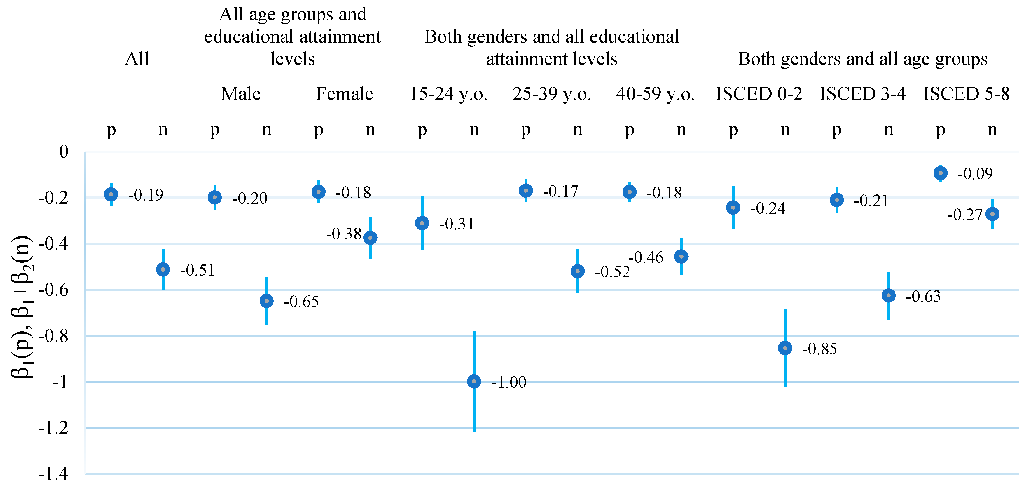
All		β1	−0.1861	(0.0228) ***	(0.0242) ***
		β1 + β2	−0.5126	(0.0462) ***	(0.0461) ***
All age groups and education levels	Male	β1	−0.1997	(0.0281) ***	(0.0279) ***
		β1 + β2	−0.6490	(0.0520) ***	(0.0515) ***
	Female	β1	−0.1750	(0.0253) ***	(0.0250) ***
		β1 + β2	−0.3751	(0.0471) ***	(0.0476) ***
All gender groups and education levels	15–24 y.o.	β1	−0.3112	(0.0602) ***	(0.0610) ***
		β1 + β2	−0.9984	(0.1120) ***	(0.1114) ***
	25–39 y.o.	β1	−0.1694	(0.0260) ***	(0.0258) ***
		β1 + β2	−0.5200	(0.0482) ***	(0.0488) ***
	40–59 y.o.	β1	−0.1755	(0.0220) ***	(0.0216) ***
		β1 + β2	−0.4560	(0.0410) ***	(0.0408) ***
All gender and age groups	ISCED 0-2	β1	−0.2432	(0.0476) ***	(0.0471) ***
		β1 + β2	−0.8541	(0.0866) ***	(0.0872) ***
	ISCED 3-4	β1	−0.2103	(0.0292) ***	(0.0218) ***
		β1 + β2	−0.6257	(0.0534) ***	(0.0527) ***
	ISCED 5-8	β1	−0.0943	(0.0186) ***	(0.0179) ***
		β1 + β2	−0.2717	(0.0335) ***	(0.0336) ***

*** indicate statistically significant at the 1% level.

,

Table A3. Robustness check of Equation (3) estimates presented in Figure 3.

Unemployment Type		Parame-ter	LSDV Estimates			2SGMM (1)
			Point Estimate of the Parameter	(Prais-Winsten std. Error)	(Newey-West std. Error)	Point Estimate of the Parameter	(Windmeijer-Corrected std. Error) (2)
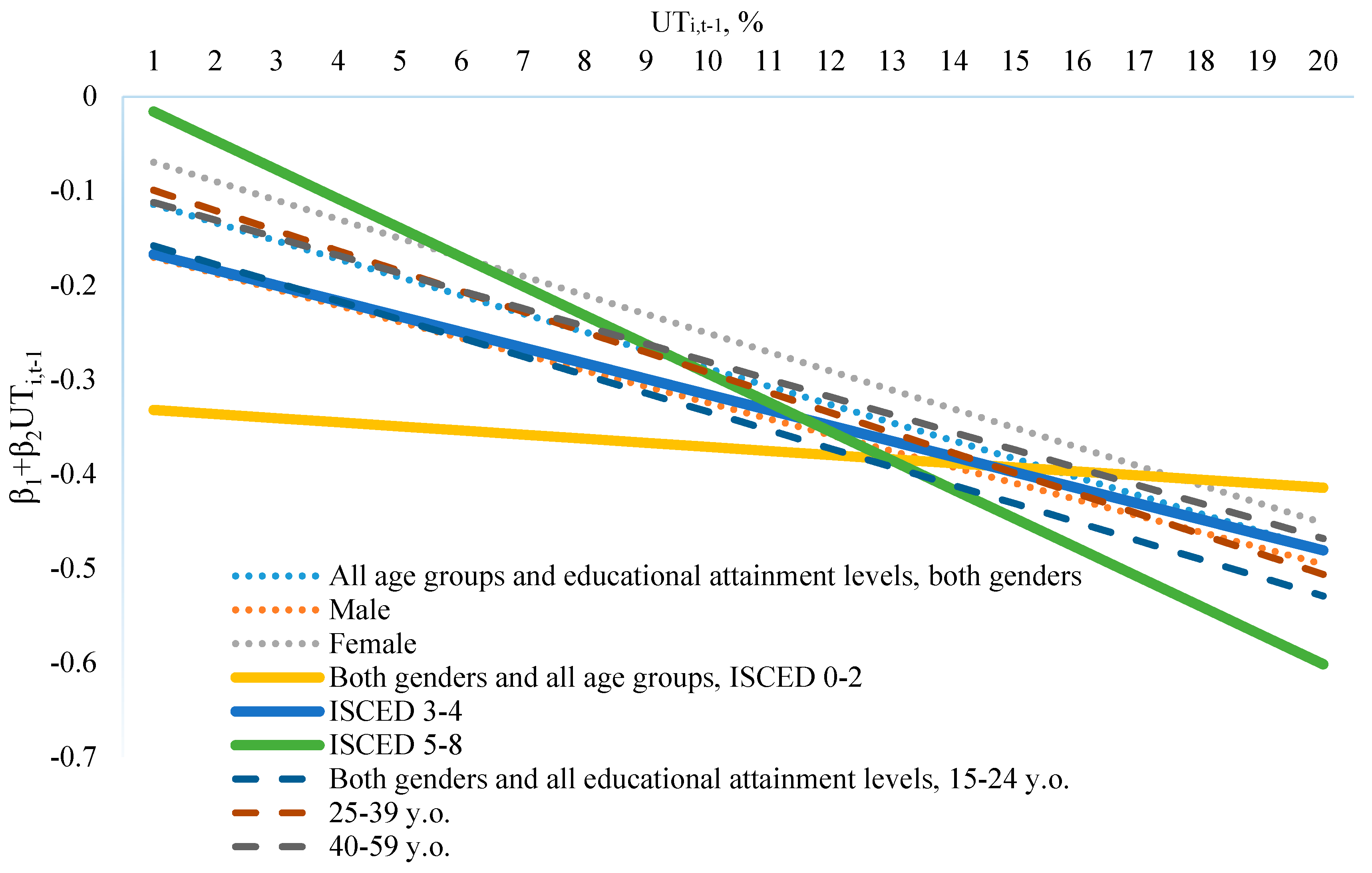
All		β1	−0.0953	(0.0398) **	(0.0394) **	−0.0978	(0.0428) **
		β2	−0.0193	(0.0036) ***	(0.0038) ***	−0.0205	(0.0033) ***
All age groups and education levels	Male	β1	−0.1534	(0.0456) ***	(0.0430) ***	−0.1545	(0.0441) ***
		β2	−0.0171	(0.0041) ***	(0.0045) ***	−0.0173	(0.0044) ***
	Female	β1	−0.0498	(0.0361)	(0.0404)	−0.0530	(0.0390)
		β2	−0.0201	(0.0032) **	(0.0038) **	−0.0205	(0.0030) **
All gender groups and education levels	15–24 y.o.	β1	−0.1388	(0.0921)	(0.0944)	−0.1460	(0.0903)
		β2	−0.0195	(0.0039) ***	(0.0035) ***	−0.0212	(0.0041) ***
	25–39 y.o.	β1	−0.0781	(0.0377) **	(0.0370) **	−0.0829	(0.0353) **
		β2	−0.0214	(0.0034) ***	(0.0036) ***	−0.0228	(0.0032) ***
	40–59 y.o.	β1	−0.0936	(0.0350) ***	(0.0359) ***	−0.0952	(0.0358) ***
		β2	−0.0187	(0.0038) ***	(0.0040) ***	−0.0185	(0.0037) ***
All gender and age groups	ISCED 0-2	β1	−0.3280	(0.0636) ***	(0.0631) ***	−0.3124	(0.0637) ***
		β2	−0.0043	(0.0032)	(0.0039)	−0.0041	(0.0031)
	ISCED 3-4	β1	−0.1507	(0.0453) ***	(0.0457) ***	−0.1403	(0.0437) ***
		β2	−0.0165	(0.0037) ***	(0.0035) ***	−0.0161	(0.0036) ***
	ISCED 5-8	β1	0.0147	(0.0229)	(0.0223)	0.0143	(0.0251)
		β2	−0.0308	(0.0034) ***	(0.0039) ***	−0.0336	(0.0034) ***

**, *** indicate statistically significant at the 5%, and 1% levels, respectively. ⁽¹⁾ Two-step generalized methods of moments (GMM) estimator that includes equations in levels. Once the 1-step estimator is computed, the sample covariance matrix of the estimated residuals is used to obtain 2-step estimates, which are not only consistent but also asymptotically efficient. ⁽²⁾ To take into account the concern of Blundell and Bond (1998) about the downward-biased tendency of standard errors estimated by the GMM approach for small samples, we used finite-sample corrections suggested by Windmeijer (2005) to the asymptotic covariance matrix of the parameters, which are nowadays almost universally used.

and

Table A4. Robustness check of Equation (4) estimates presented in Figure 4, Figure 5 and Figure 6.

Unemployment Type	Para-Meter		LSDV Estimates			2SGMM (1)
			Point Estimate of the Parameter	(Prais-Winsten std. Error)	(Newey-West std. Error)	Point Estimate of the Parameter	(Windmeijer-Corrected std. Error) (2)
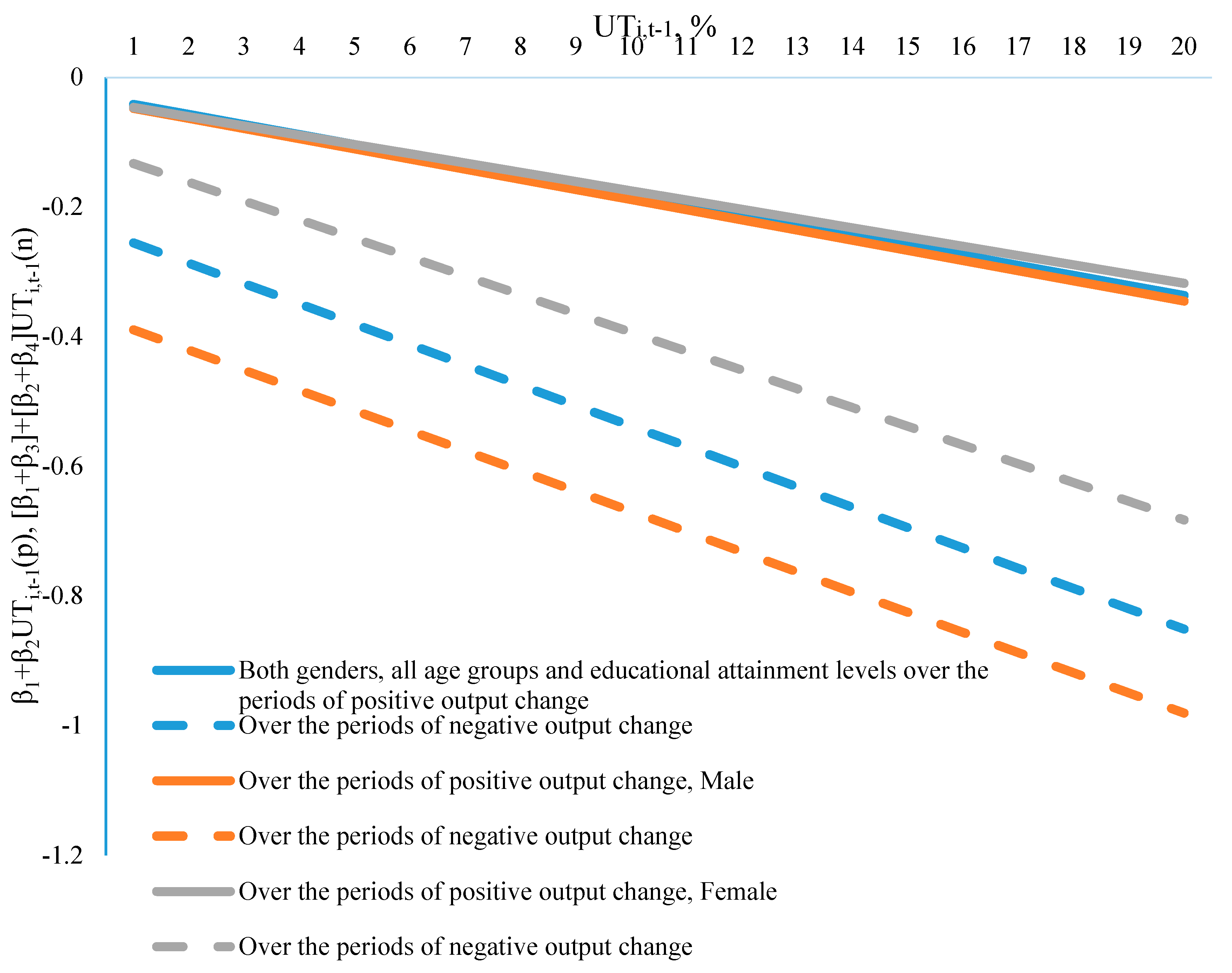
All	β1		−0.0264	(0.0526)	(0.0578)	−0.0254	(0.0524)
	β2		−0.0155	(0.0046) ***	(0.0042) ***	−0.0167	(0.0045) ***
	β1 + β3		−0.2243	(0.0861) **	(0.0822) **	−0.2135	(0.0831) **
	β2 + β4		−0.0314	(0.0086) ***	(0.0097) ***	−0.0293	(0.0086) ***
All age groups and education levels	Male	β1	−0.0324	(0.0586)	(0.0623)	−0.0293	(0.0546)
		β2	−0.0157	(0.0051) ***	(0.0049) ***	−0.0143	(0.0056) ***
		β1 + β3	−0.3586	(0.1032) **	(0.0937) **	−0.3385	(0.0963) **
		β2 + β4	−0.0311	(0.0107) ***	(0.0113) ***	−0.0316	(0.0110) ***
	Female	β1	−0.0324	(0.0508)	(0.0481)	−0.0338	(0.0464)
		β2	−0.0143	(0.0045) ***	(0.0041) ***	−0.0146	(0.0046) ***
		β1 + β3	−0.1043	(0.0765) ***	(0.0694) ***	−0.1091	(0.0808) ***
		β2 + β4	−0.0289	(0.0070) ***	(0.0073) ***	−0.0274	(0.0065) ***
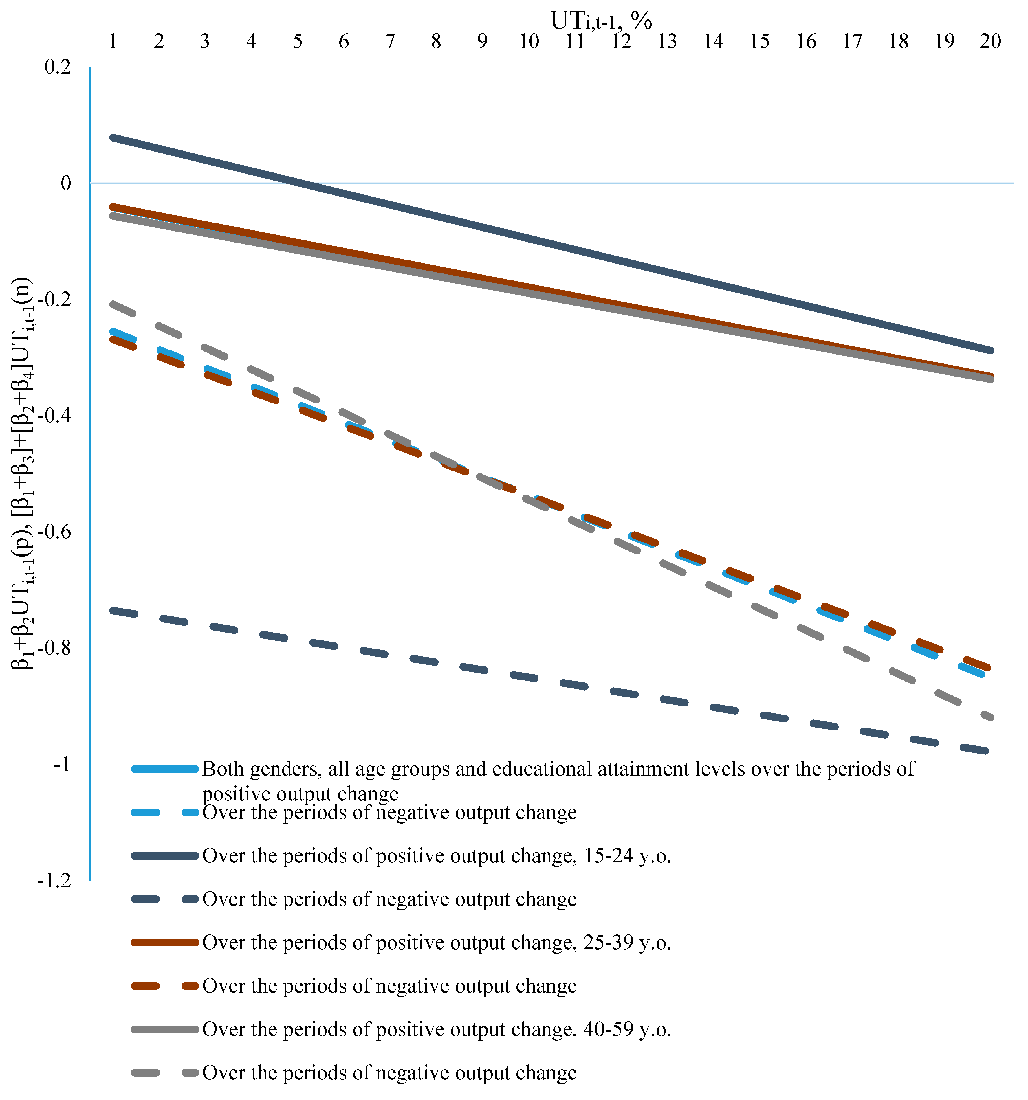
All gender groups and education levels	15–24 y.o.	β1	0.0976	(0.1260)	(0.1281)	0.0892	(0.1367)
		β2	−0.0193	(0.0055) ***	(0.0058) ***	−0.0205	(0.0055) ***
		β1 + β3	−0.7232	(0.1923) ***	(0.2050) ***	−0.6836	(0.2092) ***
		β2 + β4	−0.0128	(0.0082)	(0.0083)	−0.0129	(0.0077)
	25–39 y.o.	β1	−0.0259	(0.0507)	(0.0499)	−0.0256	(0.0464)
		β2	−0.0154	(0.0046) ***	(0.0042) ***	−0.0163	(0.0044) ***
		β1 + β3	−0.2391	(0.0783) ***	(0.0808) ***	−0.2298	(0.0812) ***
		β2 + β4	−0.0298	(0.0073) ***	(0.0072) ***	−0.0304	(0.0068) ***
	40–59 y.o.	β1	−0.0417	(0.0460)	(0.0457)	−0.0429	(0.0444)
		β2	−0.0148	(0.0048) ***	(0.0051) ***	−0.0147	(0.0043) ***
		β1 + β3	−0.1712	(0.0829) **	(0.0841) **	−0.1686	(0.0810) **
		β2 + β4	−0.0374	(0.0104) ***	(0.0101) ***	−0.0398	(0.0113) ***
All gender and age groups	ISCED 0-2	β1	−0.1012	(0.0876)	(0.0931)	−0.1105	(0.0947)
		β2	−0.0068	(0.0042)	(0.0046)	−0.0074	(0.0043)
		β1 + β3	−0.6787	(0.1594) ***	(0.1623) ***	−0.6588	(0.1701) ***
		β2 + β4	−0.0106	(0.0098)	(0.0096)	−0.0111	(0.0092)
	ISCED 3-4	β1	−0.0556	(0.0583)	(0.0611)	−0.0601	(0.0621)
		β2	−0.0136	(0.0046) ***	(0.0049) ***	−0.0133	(0.0043) ***
		β1 + β3	−0.3381	(0.0986) ***	(0.1055) ***	−0.3199	(0.1068) ***
		β2 + β4	−0.0272	(0.0089) ***	(0.0082) ***	−0.0263	(0.0094) ***
	ISCED 5-8	β1	0.0042	(0.0317)	(0.0293)	0.0041	(0.0315)
		β2	−0.0193	(0.0050) ***	(0.0054) ***	−0.0200	(0.005) ***
		β1 + β3	−0.0186	(0.0487)	(0.0500)	−0.0190	(0.0448) ***
		β2 + β4	−0.0432	(0.0070) ***	(0.0075) ***	−0.0407	(0.0067) ***

**, *** indicate statistically significant at the 5%, and 1% levels, respectively. ⁽¹⁾ Two-step generalized methods of moments (GMM) estimator that includes equations in levels. Once the 1-step estimator is computed, the sample covariance matrix of the estimated residuals is used to obtain 2-step estimates, which are not only consistent but also asymptotically efficient. ⁽²⁾ To take into account the concern of Blundell and Bond (1998) about the downward-biased tendency of standard errors estimated by the GMM approach for small samples, we used finite-sample corrections suggested by Windmeijer (2005) to the asymptotic covariance matrix of the parameters, which are nowadays almost universally used.

.

Estimates using alternative standard errors to address serial correlation and heteroscedasticity problems result in the same significance of the estimated Okun’s coefficients, thus our conclusions based on LSDV estimates with Newey–West standard errors are left unchanged. Considering the application of the Arellano–Bond estimator on Equation (3) with the specification that introduced dynamics in the panel data, the estimated reaction of unemployment on growth for males and females and among different age groups became less distinct but more different considering educational attainment level-specific unemployment. Estimates using Equation (4) show that differences in the reaction compared to general estimates are bigger over economic downturns compared to upturns. This shows that educational attainment level should be considered as the important factors affecting the size of Okun’s coefficient and especially during economic decline.

Our results confirm asymmetric age-, gender- and educational attainment level-specific unemployment reactions over the business cycle. Therefore, studies that do not distinguish between growth and decline stages provide an inaccurate estimate of the unemployment rate response to an output change.

5. Conclusions

The relationship between economic growth and unemployment has been widely discussed in the scientific literature; however, significant variation of the Okun’s coefficient across countries raises the question of what are the factors influencing the heterogeneity of the coefficient. The literature review suggests that Okun’s coefficient variation can be related to gender, age and educational attainment level. The magnitude of gender-specific Okun’s coefficient suggests higher unemployment sensitivity to the business cycle for males than females, while as empirical evidence confirms that youth unemployment responds more strongly to output fluctuations compared to their older counterparts. Despite the extensive literature on the output–unemployment relationship, there is a lack of empirical evidence on how education level influences the situation of workers in the labour market over the business cycle.

Variation of Okun’s coefficient during the business cycle is usually analysed splitting the sample into periods for positive and negative output change or introducing interaction between output change and a dummy that indicates whether a change is positive or negative. We extend this approach by suggesting using overall unemployment over the previous period as a proxy for the depth of the business cycle phase. This allows us to estimate an Okun’s coefficient that is conditional and different for early or late expansion, the beginning of the downturn and deep crisis.

Our estimates suggest that unemployment’s reaction to the output change is asymmetric, i.e., higher when output is decreasing and lower when it is increasing. The same holds for gender-, age- and educational attainment level-specific unemployment. We also find that Okun’s coefficients are moderated by the level of the overall unemployment. However, this is true only during the economic downturn, i.e., the higher the overall unemployment, the bigger the negative effect on unemployment a further output decrease will have. Meanwhile, during the periods of positive output change, Okun’s coefficient is small and does not change much with the decrease in overall unemployment. This means that expansive economic policy aimed to increase total expenditures and output has a limited effect on unemployment, and it remains almost the same regardless of the level of the overall unemployment.

Our findings support the view that the reaction of youth and male unemployment to output change stands out. However, we have empirical evidence that this is true only over the periods of negative output change, while during economic upturns, there are no statistically significant differences between Okun’s coefficients for males and females or for different age groups. However, this is not the case considering educational attainment level-specific unemployment, which was not previously researched in this context. Unemployment for tertiary-educated people reacts significantly less to an output change compared to the low-and middle-educated, suggesting evidence that education is another important factor next to gender and age in explaining the heterogeneity of Okun’s coefficients.

Low-educated youths and especially males are mostly affected by the economic downturn during its initial phase. Over time, when the overall unemployment will increase, i.e., the recession becomes deeper, the reaction of other specific types of unemployment to negative output change will sharply increase and becomes similar. It means that we can expect to observe a significantly different Okun’s coefficient and thus unemployment reactions to an output change not over the whole period of the recession, but mostly during its initial stage.

Our future research can be conducted in two main directions: (i) deepening the results of the aspects evaluated in this study, applying additional methods, i.e., threshold autoregressive model which allows distinguishing threshold level where the sensitivity of unemployment rate to economic growth/decline changes its nature, speed, strength, etc.; (ii) widening the research field to how the sensitivity of unemployment to economic growth differs between countries in different regions of the EU, how this phenomenon depends on economic structure, institutional labour market regulation and the changes in labour market flows, related to migration, educational enrolment, and size of the labour force.

References

- Aaronson, Stephanie R., Mary C. Daly, William L. Wascher, and David W. Wilcox. 2019. Okun Revisited: Who Benefits Most from a Strong Economy? Brookings Papers on Economic Activity 1: 333–404. [Google Scholar] [CrossRef]
- Aguiar-Conraria, Luís, Manuel M. F. Martins, and Maria Joana Soares. 2020. Okun’s Law Across Time and Frequencies. Journal of Economic Dynamics and Control 116: 1–15. [Google Scholar] [CrossRef]
- Ahn, JaeBin, Zidong An, John C. Bluedorn, Gabriele Ciminelli, Zsoka Koczan, Davide Malacrino, Daniela Muhaj, and Patricia Neidlinger. 2019. Work in progress: Improving youth labor market outcomes in emerging market and developing economies. IMF Staff Discussion Note 2019. [Google Scholar] [CrossRef]
- Askenazy, Philippe, Martin Chevalier, and Christine Erhel. 2015. Okun’s Laws differentiated by Education. Document de travail CEPREMAP 1514. Available online: https://pdfs.semanticscholar.org/070d/d14a6226216d918b6053539537d76b91e90a.pdf (accessed on 19 July 2020).
- Bachmann, Ronald, and Mathias Sinning. 2016. Decomposing the Ins and Outs of Cyclical Unemployment. Oxford Bulletin of Economics and Statistics 78: 853–76. [Google Scholar] [CrossRef]
- Balakrishnan, Ravi, Mitali Das, and Prakash Kannan. 2010. Unemployment dynamics during recessions and recoveries:Okun’s law and beyond. IMF World Economic Outlook 69108. Available online: file:///C:/Users/MDPI/AppData/Local/Temp/_c3pdf.pdf (accessed on 1 July 2020).
- Ball, Laurence M., Daniel Leigh, and Prakash Loungani. 2013. Okun’s Law: Fit at Fifty? National Bureau of Economic Research Working Paper 18668. Available online: https://www.nber.org/papers/w18668.pdf (accessed on 1 July 2020).
- Ball, Laurence M., Daniel Leigh, and Prakash Loungani. 2017. Okun’s law: Fit at 50? Journal of Money, Credit and Banking 49: 1413–41. [Google Scholar] [CrossRef]
- Ball, Laurence M., Davide Furceri, Daniel Leigh, and Prakash Loungani. 2019. Does one law fit all? Cross-country evidence onOkun’s law. Open Economies Review 30: 841–74. [Google Scholar] [CrossRef]
- Banerji, Angana, Sergejs Saksonovs, Huidan Lin, and Rodolphe Blavy. 2014. Youth unemployment in advanced economies in Europe: Searching for solutions. IMF Staff Discussion Note 14. [Google Scholar] [CrossRef]
- Banerji, Angana, Huidan Lin, and Sergejs Saksonovs. 2015. Youth unemployment in advanced Europe: Okun’s law and beyond. IMF Working Paper 15. [Google Scholar] [CrossRef]
- Baussola, Maurizio, and Chiara Mussida. 2017. Regional and gender differentials in the persistence of unemployment in Europe. International Review of Applied Economics 31: 173–90. [Google Scholar] [CrossRef]
- Belaire-Franch, Jorge, and Amado Peiró. 2015. Asymmetry in the relationship between unemployment and the business cycle. Empirical Economics 48: 683–97. [Google Scholar] [CrossRef]
- Benda, Luc, Ferry Koster, and Romke J. van der Veen. 2019. Levelling the playing field? Active labour market policies, educational attainment and unemployment. International Journal of Sociology and Social Policy 39: 276–95. [Google Scholar] [CrossRef]
- Blundell, Richard, and Stephen Bond. 1998. Initial conditions and moment restrictions in dynamic panel data models. Journal of Econometrics 87: 115–43. [Google Scholar] [CrossRef]
- Brambor, Thomas, William Roberts Clark, and Matt Golder. 2006. Understanding Interaction Models: Improving Empirical Analyses. Political Analysis 14: 63–82. [Google Scholar] [CrossRef]
- Bredtmann, Julia, Sebastian Otten, and Christian Rulff. 2018. Husband’s Unemployment and Wife’s Labor Supply: The Added Worker Effect across Europe. ILR Review 71: 1201–31. [Google Scholar] [CrossRef]
- Breen, Richard. 2005. Explaining cross-national variation in youth unemployment: Market and institutional factors. European Sociological Review 21: 125–34. [Google Scholar] [CrossRef]
- Brincikova, Zuzana, and Lubomir Darmo. 2015. The impact of economic growth on gender specific unemployment in the EU. Scientific Annals of the “Alexandru Ioan Cuza” University of Iaşi Economic Sciences 62: 383–90. [Google Scholar] [CrossRef]
- Brunello, Giorgio, Pietro Garibaldi, Etienne Wasmer, and Andrea Bassanini. 2007. Education and Training in Europe. Oxford: Oxford University Press. [Google Scholar]
- Butkus, Mindaugas, and Janina Seputiene. 2019. The Output Gap and Youth Unemployment: An Analysis Based on Okun’s Law. Economies 7: 108. [Google Scholar] [CrossRef]
- Dellas, Harris, and Plutarchos Sakellaris. 2003. On the cyclicality of schooling: Theory and evidence. Oxford Economic Papers 55: 148–72. [Google Scholar] [CrossRef]
- Devereux, Paul J. 2002. Occupational upgrading and the business cycle. Labour 16: 423–52. [Google Scholar] [CrossRef]
- Dietrich, Hans, and Joachim Möller. 2016. Youth unemployment in Europe—business cycle and institutional effects. International Economics and Economic Policy 13: 5–25. [Google Scholar] [CrossRef]
- Dixon, Robert, Guay C. Lim, and Jan C. van Ours. 2017. Revisiting the Okun relationship. Applied Economics 49: 2749–65. [Google Scholar] [CrossRef][Green Version]
- Dunsch, Sophie. 2016. Okun’s law and youth unemployment in Germany and Poland. International Journal of Management and Economics 49: 34–57. [Google Scholar] [CrossRef]
- Dunsch, Sophie. 2017. Age- and gender-specific unemployment and Okun’s law in CEE countries. Eastern European Economics 55: 377–93. [Google Scholar] [CrossRef]
- Estevão, Marcello M., and Evridiki Tsounta. 2011. Has the Great Recession raised US structural unemployment? IMF Working Papers 11: 1–46. Available online: https://ssrn.com/abstract=1847338 (accessed on 1 July 2020).
- European Commission. 2013. Labour market developments in Europe 2013. European Economy 6. [Google Scholar] [CrossRef]
- Evans, Andrew. 2018. Okun coefficients and participation coefficients by age and gender. IZA Journal of Labor Economics 7: 1–22. [Google Scholar] [CrossRef]
- Fontanari, Claudia, Antonella Palumbo, and Chiara Salvatori. 2020. Potential output in theory and practice: A revision and update of Okun’s original method. Structural Change and Economic Dynamics 54: 247–66. [Google Scholar] [CrossRef]
- García, Amparo Nagore. 2017. Gender Differences in Unemployment Dynamics and Initial Wages over the Business Cycle. Journal of Labor Research 38: 228–60. [Google Scholar] [CrossRef]
- Garrouste, Christelle, Kornelia Kozovska, and Elena Arjona Perez. 2010. Education and long-term unemployment. MPRA Paper 25073: 1–29. Available online: https://mpra.ub.uni-muenchen.de/25073/1/MPRA_paper_25073.pdf (accessed on 1 July 2020).
- Guisinger, Amy Y., Ruben Hernandez-Murillo, Michael T. Owyang, and Tara M. Sinclair. 2018. A state-level analysis of Okun’s law. Regional Science and Urban Economics 68: 239–48. [Google Scholar] [CrossRef]
- Huang, Gang, Ho-Chuan Huang, Xiaojian Liu, and Jiangang Zhang. 2020. Endogeneity in Okun’s law. Applied Economics Letters 27: 910–14. [Google Scholar] [CrossRef]
- Hutengs, Oliver, and Georg Stadtmann. 2013. Age effects in the Okun’s law within the Eurozone. Applied Economics Letters 20: 821–25. [Google Scholar] [CrossRef]
- Hutengs, Oliver, and Georg Stadtmann. 2014a. Age- and gender-specific unemployment in Scandinavian countries: An analysis based on Okun’s law. Comparative Economic Studies 56: 567–80. [Google Scholar] [CrossRef]
- Hutengs, Oliver, and Georg Stadtmann. 2014b. Don’t trust anybody over 30: Youth unemployment and Okun’s law in CEE countries. Bank and Credit 45: 1–16. [Google Scholar]
- Kim, Myeong Jun, and Sung Y. Park. 2019. Do gender and age impact the time-varying Okun’s law? Evidence from South Korea. Pacific Economic Review 24: 672–85. [Google Scholar] [CrossRef]
- Kim, Jun, Jong Cheol Yoon, and Sang Young Jei. 2020. An empirical analysis of Okun’s laws in ASEAN using time-varying parameter model. Physica A: Statistical Mechanics and its Applications 540: 2–9. [Google Scholar] [CrossRef]
- Marconi, Gabriele, Miroslav Beblavý, and Ilaria Maselli. 2016. Age effects in Okun’s law with different indicators of unemployment. Applied Economics Letters 23: 580–83. [Google Scholar] [CrossRef]
- Melina, Giovanni, and Jose Torres. 2016. Enhancing the Responsiveness of Employment to Growth in Namibia. IMF Country Report 16. Available online: https://www.imf.org/external/pubs/ft/scr/2016/cr16374.pdf (accessed on 15 June 2020).
- Micallef, Brian. 2016. Empirical estimates of Okun’s Law in Malta. Applied Economics and Finance 4: 138–48. [Google Scholar] [CrossRef][Green Version]
- Modestino, Alicia Sasser, Daniel Shoag, and Joshua Balance. 2016. Downskilling: Changes in Employer Skill Requirements over the Business Cycle. Labour Economics 41: 333–47. [Google Scholar] [CrossRef]
- Nebot, César, Arielle Beyaert, and José García-Solanes. 2019. New insights into the non-linearity of Okun’s law. Economic Modelling 82: 202–10. [Google Scholar] [CrossRef]
- Novák, Marcel, and Ľubomír Darmo. 2019. Okun’s law over the business cycle: Does it change in the EU countries after the financial crisis? Prague Economic Papers 28: 235–54. [Google Scholar] [CrossRef]
- Oh, Jong-seok. 2017. Changes in cyclical patterns of the USA labor market: From the perspective of non-linear Okun’s law. International Review of Applied Economics 32: 237–58. [Google Scholar] [CrossRef]
- Okun, Arthur M. 1962. Potential GNP: Its measurement and significance. In Proceedings of the Business and Economics Section. Edited by the American Statistical Association. Washington, DC: American Statistical Association, pp. 98–104. [Google Scholar]
- Owyang, Michael T., and Tatevik Sekhposyan. 2012. Okun’s law over the business cycle: Was the great recession all that different? Federal Reserve Bank of St. Louis Review 94. Available online: http://citeseerx.ist.psu.edu/viewdoc/download?doi=10.1.1.259.3698&rep=rep1&type=pdf (accessed on 15 June 2020).
- Scarpetta, Stefano, Anne Sonnet, and Thomas Manfredi. 2010. Rising youth unemployment during the crisis: How to prevent negative long-term consequences on a generation? OECD Social, Employment and Migration Papers 106. [Google Scholar] [CrossRef]
- Tang, Bo, and Carlos Bethencourt. 2017. Asymmetric unemployment-output tradeoff in the Eurozone. Journal of Policy Modeling 39: 461–81. [Google Scholar] [CrossRef]
- Vermann, E. Katarina, and Michael T. Owyang. 2013. Okun’s law in recession and recovery. Economic Synopses. Available online: https://files.stlouisfed.org/files/htdocs/publications/es/13/ES_23_2013-08-16.pdf (accessed on 15 June 2020).
- Vuolo, Mike, Jeylan T. Mortimer, and Jeremy Staff. 2016. The value of educational degrees in turbulent economic times: Evidence from the youth development study. Social Science Research 57: 233–52. [Google Scholar] [CrossRef] [PubMed]
- Windmeijer, Frank. 2005. A finite sample correction for the variance of linear efficient two-step GMM estimators. Journal of Econometrics 126: 25–51. [Google Scholar] [CrossRef]
- World Bank. 2012. Gender differences in employment and why they matter. World Development Report, 198–253. [Google Scholar] [CrossRef]
- Zanin, Luca. 2014. On Okun’s law in OECD countries: An analysis by age cohorts. Economics Letters 125: 243–48. [Google Scholar] [CrossRef]
- Zanin, Luca. 2018. The pyramid of Okun’s coefficient for Italy. Empirica 45: 17–28. [Google Scholar] [CrossRef]