Abstract
Political unrest inevitably has consequences for a national economy. International trade in a globalised world has great importance for countries. Unfortunately, due to various political events, countries apply some restrictions to each other. In 2014, Western countries imposed sanctions on trade with Russia, due to the annexation of Crimea. As a response, Russia announced an embargo on importing of some goods from European and North American countries, as well as Australia. The current study investigates the economic impact on EU countries due to the mentioned embargo. The EU countries were grouped according to the average for 1998–2018 exports of products to Russia using a cluster analysis. After the clustering, the gravity model was employed to develop the equations representing the international trade between each cluster and Russia. Although Russia declared an embargo on countries associated with the same group of goods, the economic impact on their economies was different. This study has a couple of limitations. The research reflects only the impact of the embargo on exports regardless of some possible indirect effects; the study assesses the export of all sectors due to limited data; and because the restrictions are applied only to the food sector, the research shows only relative changes in exports.
Keywords:
embargo; embargo impact on economy; international trade; political decisions; cluster analysis; gravity model JEL Classification:
F1; F51; F62
1. Introduction
Political decisions have been examined by a wide range of scholars from different fields of science. It is a broad topic, as political decisions can change the political situation of a country, and they are also tightly linked to the economic situation of that country as well. Hence, the impact of political decisions is a topic gaining higher interest from the scientific community. For instance, there are scientists who have investigated the influence of political decisions on the performance of investment funds (Witkowska et al. 2019; García Costa et al. 2019). Other scholars have sought to find out if there was an interface between political decisions and macroeconomic variables (Tkáčová et al. 2018; Battaglini and Coate 2008; Sasongko and Huruta 2018). Furthermore, the impact of political decisions on economic relations between countries has also been examined (Maxim and van der Sluijs 2011; Gil-González et al. 2008). However, studies that have analysed the influence of political decisions on economic relations were conducted some time ago and were fragmented. Hence, there is a gap in the scientific knowledge because current situations regarding the interface between economic relations and political decisions have been unexplored. One such field is Russia’s embargo, which is a political decision that has changed the situation in world trade. The European Union and the United States of America imposed sanctions on Russia, in 2014, due to the annexation of Crimea, and, in response, Russia announced the embargo on the import of some goods from the EU countries, Norway, the USA, Australia, and Canada. The current topic is not widely investigated in the scientific literature and there are only a few evidences of the embargo impact on international trade between the countries mentioned above, although international trade has been researched by many scientists (e.g., Yang and Nie 2020; Ge et al. 2019; Wang and Kong 2019).
The investigation of the Russian embargo helps to determine the impact the restrictions have on trade between nations. We analysis the embargo of Russia on the EU countries represented in this paper. The theoretical framework helps to understand the interaction between political decisions and economic relations. In addition, based on a review of scientific articles we can divide the political decisions that affect economic ties into groups. For the analysis, the research examines the statistics on export, gross domestic product, population, the distance between capitals, and common borders of the EU countries and Russia. This paper shows the impact of Russia’s embargo on EU countries economy using statistics. It is believed that the Russian embargo on its imports has a different effect on exports from the various EU countries. This study assesses the changes in total exports of EU counties, notwithstanding the embargo imposed on only some products. The EU countries were able to launch active trade with Russia for products that were not subject to this embargo, thus, compensating export losses, by adapting to market conditions. Hence, the current research aims to evaluate the impact of Russia‘s embargo on the economies of the EU countries based on an investigation of the effect of a political decision such as Russia’s embargo on economic relations with the EU countries expressed through the export volume.
2. Theoretical Background
International relations deal with the foreign policy of the states within the framework of a global system, including the influence of international organisations, non-governmental organisations, and international corporations, as well as other aspects of relations between states. International relations theories are based on various social sciences disciplines, i.e., political science, economics, history, law, philosophy, and sociology (Hodder 2017). There are many examples of political decisions that have changed the economic relations of a state. Politicians make economical modifications by changing laws, setting taxes, customs or quotas, and also by imposing embargos or sanctions. Moreover, the government can provide compensations, scholarships, or other promotions to increase some economic sector or indicator of the state.
The analysis of international economic relationships is essential for understanding how they could be expressed and what indicators reflect them. The leading indicator, which summarises the development of a country’s economy, is the gross domestic product (GDP) (Stremousova and Buchinskaia 2019). The GDP is also an essential indicator for analysing inflation. In other words, usually, the higher the GDP, the higher the inflation rate is. “Under annual inflation targeting (IT), the full impact of adverse supply shocks is felt as lost real GDP” (Bhandari and Frankel 2017). The GDP growth stimulates the supply. Hence, the GDP is still one of the most critical indicators for analysing a country’s economy, and various political decisions could influence its changes.
The external sector and foreign trade are the most prestigious groups of indicators for the analysis of international relations. These indicators consist of the current account balance, the export of goods, the annual change in the export of products, the import of goods, the annual change in the import of goods, and the foreign direct investment (Official Statistic Portal 2019).
One more factor that could have an impact on export is government regulations. An analysis by Dou et al. (2015) showed that domestic and also foreign policy could influence trading. Their research on the relationship between trades of food and food safety set by the importing countries and the exporting country showed that some prohibitions and restrictions by importing countries harm an exporting country’s exports (Dou et al. 2015). Some political decisions, such as trade agreements, can have a positive impact on trading for both importing and exporting countries. An excellent example of it is the North American Free Trade Agreement (NAFTA). The relationship between the USA and Mexico became better after signing the NAFTA, and the export of both countries increased (Bejan 2011). Some agreements do not exist for a long time. Moreover, changes in the government of countries can modify the volume of export drastically.
Imports are also an important indicator for analysing economic relations between countries. Imports could offer access to the newest technology and inputs combination, which, in turn, could lead to developing a new product or improving an existing product to export (Castellani and Fassio 2019). Imports help a country to be more globalised and to enhance some sectors. Additionally, consumers have a more extensive range of products and a more comprehensive range of prices. However, the government protects the domestic market from big foreign competitors by imposing duties or tariffs. The import of final goods is always taxed to extract and shift rents from international firms, while the import of intermediate goods could be both taxed or subsidised (Wang et al. 2011).
Moreover, Wang et al. (2011) found that a charge on final goods could both increase and decrease the domestic price of those goods. Local producers gain benefits after the introduction of custom duties. They fill the demand by expanding their production. Furthermore, as the prices of imported products rise, they can raise their rates to the level of the customs’ guarantee and gain higher profits. In summary, imports give benefits by providing better quality goods and services and widening the range of choices, but if imports exceed exports, a country suffers losses.
Some political decisions only impact the national economy, but sometimes they also affect global economic relations. The interface between political decisions and the economy can be expressed in different ways. Some political decision can affect the indicators of a country’s national and international economic relations either positively or negatively. One of the decisions that can significantly influence economic relations is related to sanctions or embargos. Venkuviene and Masteikiene (2015) researched how the economic embargo by the Russian Federation affected the European economy and economic relations. They found that it changed the economies of CEE (Central and Eastern European) countries negatively, i.e., the export of dairy and meat sectors fell (main sectors in CEE countries that collect most of the GDP). Similarly, expedition and logistic companies felt significant losses (Venkuviene and Masteikiene 2015).
Furthermore, Gharehgozli (2017) analysed the United States sanctions on Iran. The results showed that they reduced Iran’s real GDP by more than 17% (Gharehgozli 2017). Another example of sanctions would be the Western financial sanctions on the Russian Federation which were analysed by Gurvich and Prilepskiy (2015). The sanctions decreased foreign direct investment in the Russian Federation. In addition, there were fewer borrowing opportunities for companies and banks not directly targeted by the sanctions and lower capital inflow into the government debt market.
Moreover, the drop in prices led to GDP losses of 8.5% (Gurvich and Prilepskiy 2015). Furthermore, the United Nations and the United States economic sanctions on target states harmed the economy too. The sanctions reduced the annual real per capita GDP growth rate by more than 2% and led to an aggregate decline in GDP of 25.5% (Neuenkirch and Neumeier 2015).
Political decisions can also affect currency which is also essential for foreign trade. Orăştean (2013) analysed the decision by China and Japan to use only the yen and yuan in bilateral trade. It turned out that this decreased the value of the dollar (Orăştean 2013). It cannot be concluded that all these political decisions were made to negatively impact the economy and economic relations of other countries. It should be highlighted that political decisions that harm economic relations can have a positive effect in another field.
Nevertheless, some political decisions have a positive effect on the economy and economic relations. Monticelli et al. (2017) give an example about institutions in Brazil that were created and played an important role in the development and consolidation of the wine industry, also fostered relationship strategies that were based on the participation of wineries and its internationalisation. It helped to promote and improve the winery industry and boost foreign trade. Another political decision that has a significant positive impact on economic relations is related to agreements and organisations. Nápoles (2017) conducted research on how Mexico’s accession into the North American Free Trade Agreement (NAFTA) impacted its economy and economic relations. The results showed that Mexico’s GDP increased from 1.7% to 2.6%, GDP per capita increased from −0.4% to 1.2% and export increased from 6.1% to 8.4% (Nápoles 2017). Another free trade agreement was made between the EU and Canada that eradicated 6.5% of import duties (Hübner 2016).
A government also makes some different decisions to improve its economy, economic relations, or society. Imbruno (2016) explained the decision of China that began a process of phasing out the quantitative planning of trade flows and reformed its trade regime using conventional policy instruments, such as tariffs and quotas. The process had a positive effect because the average tariff rate decreased from 56% to 15%, the share of imports under quota/license regulation fell to 8.5%, and the number of firms with the right to trade abroad increased from “twelve state-owned firms” to 35,000 (Imbruno 2016). In addition, a government controls tariffs and duties a lot and sometimes it affects foreign countries. According to Mitra and Shin (2012), tariff reductions in China increased firm-level labour-demand elasticity in Korea. Moreover, the liquefied natural gas (LNG) import quota introduced in Lithuania decreased natural gas prices (Schulte and Weiser 2019). All political decisions are made to somehow improve the level of the economy, economic relations, or society in a country, as well as relationships with other countries.
However, some political decisions have both negative and positive impacts. One of the significant political decisions was the introduction of the euro in Lithuania. The introduction of the euro in the short term positively impacted the growth of Lithuania’s international trade and the reduction of interest rates and the most significant negative influence of the introduction of the euro was linked to the growth of inflation and price levels (Januškevičius 2017). Moreover, the rise of excise duty for alcohol and cigarettes and change of the alcohol control law in Lithuania also had positive and negative impacts. Alcohol and tobacco prices increased, and this reduced the level of trade. However, consumption of alcohol decreased by about 2% which meant a better standard of society’s health (The Department of Statistics of the Republic of Lithuania 2017).
It can be concluded that almost all political decisions have positive and negative impacts. Nevertheless, sometimes the effect is minimal, and therefore it seems that the influence of a decision is only positive or negative.
On the basis of the analysed information, we can divide the impact of political decisions into groups (Table 1). The impact can be negative, positive, or both negative and positive. Moreover, political decisions can have an impact at a national, global, or national and global level, as well as an effect on the economy, society, or relations with other countries.

Table 1.
Possible impacts of political decisions on various indicators (designed by authors).
After the analysis of theoretical aspects of the influence of political decisions on a country’s economic relations, we can conclude that economic relations and politics are strongly related all the time. It is possible to analyse economic relations through economic indicators such as gross domestic product (GDP), imports, exports, and others. According to the scientific articles, it is possible to group political decisions as follows: agreements and memberships in organisations, embargos and sanctions, help for local businesses, and changes in domestic policy. Political decisions can have negative, positive, or both negative and positive impacts. Moreover, political decisions can have an effect at a national, global, or national and global level, as well as on the economy, society, or relations with other countries.
3. Methodology
In order to more precisely investigate the international trade between the EU and Russia, a cluster analysis was performed. The purpose of cluster analysis was to identify the relatively homogeneous groups of the EU countries based on the average of exports to Russia for 1998–2018. For the purpose of assessing the level of dissimilarities across the EU countries, a cluster analysis based on hierarchical ascendant classification (HAC) was implemented. The first step of the HAC procedure was estimation of the dissimilarities between any pair of objects (Coudert et al. 2020), or in the current case, countries. The similarity coefficient is defined by the Euclidean distance between country i and country j:
where is the Euclidean distance between Xi and Xj, Xi,t is the average export to Russia from country i at period t (t = T1, …, TN), and Xj,t is the average export to Russia from country j at period t (t = T1, …, TN).
For cthe lustering procedure, Ward’s linkage was selected as the agglomerative method. Ward’s linkage is based on the distance between the centroids of two clusters (Coudert et al. 2020):
where is the distance between the centroids of the two clusters and; A and B are clusters; and nA, nB is the number of objects within the clusters.
After the cluster analysis was performed, the gravity model was selected to investigate the international trade between each cluster and Russia. The gravity model is a mathematical model based on Newton’s gravitational theory, that states that “the gravitational force between two bodies is proportional to the product of their masses and inversely proportional to the square of the distance between them” (Knox 2011). Usually, the model is used to research import and export issues (Nguyen 2019; Pinilla and Rayes 2019; Shahriar et al. 2019; Riedel and Slany 2019).
The traditional gravity equation explains the bilateral trade flow between countries and is expressed by the following equation (Anderson 2011):
where Xij is the bilateral trade flow from country i to country j, Yi is the economic dimensions of the country I, Yj is the economic dimensions of the country j, and dij is the distance between countries i and j
Following the econometric evaluation of the traditional gravity equation, new variables are included in the equation (Fetahu 2014):
Xij is the volume of trade between the two countries and , Yi is the economic indicator of country I, Yj is the economic indicator of country j, dij is the distance between countries and , G is Constanta, and nij is the error term with expectation equal to 1.
The Mellor (1964) gravity model equation was expressed by using the traditional gravity model equation in the calculation of bilateral trade flows by the natural logarithmic function in order to get more accurate results (Doumbe and Belinga 2015):
where Xij is a dependent variable; α0, α1, α2, α3 are coefficients; and Xi, Xj, dij are independent variables.
According to the theory of gravity equation, an initial gravity equation is proposed, based on which regression analysis is performed:
where:
Et is the export volumes of the European Union products to Russia. The export data variable in the research is the size of the European Union export as a whole and the export size of each European Union country in thousands of dollars.
EUGDPt is the Gross domestic product of the EU countries. This variable in the research is understood as the gross domestic product of the European Union as a whole or individual EU country in billions of dollars. It is assumed that larger countries tend to be more active in international trade than smaller countries, taking into account the theory of international trade.
RUGDPt is the Russian gross domestic product. EU exports are believed to be influenced by Russia’s macroeconomic situation, which is reflected in GDP.
Popt is the population of the EU countries, which allows one to evaluate the size of the market of each country. Countries with more populations are expected to be more active in international trade, but according to the theory of international trade, larger countries may be reluctant to export much.
Km is distance. The variable between countries expresses the geographical distance of the capitals of the 28 EU countries to the Russian capital Moscow. According to the gravity model theory, the further the distance, the smaller the trade, because of transport costs, the convenience of transportation and the closer markets, closer countries are more active in trade.
Bor is a common EU country’s border with Russia. This fictitious variable (called pseudo-variable in scientific literature) is expressed as 0 (the country has no common border with Russia) or 1 (the country has a common border with Russia). Countries with a common border are expected to be more active in cross-border trade than countries that do not have a common border.
The expected signs of the slopes are presented in Table 2.
Table 2.
Expected values of the variables of the gravity equation (designed by author).
All the variables of the gravity equation are logarithmic. Although the gravity equation is written as a log-log function but based on gravity theory, this function is analysed as a linear regression equation. Various methods are used in the research for regression analysis of the gravity equation. The gravity model significance assessment is made by using the least-squares method, which allows one to estimate the coefficients of independent variables and the significance of the model by minimising residual errors.
In order to test the validity of the developed equations, several tests were used. In order to test if the data were normally distributed, Kolmogorov–Smirnov and Shapiro–Wilk tests were employed. The Kolmogorov–Smirnov test is the most frequently used test of normality and could be written as follows (Steinskog et al. 2007):
where d is the Kolmogorov–Smirnov statistic, is the cumulative population distribution under the null hypothesis H0 represents an empirical cumulative distribution function.
The Shapiro–Wilk statistic could be defined as a ratio of the best estimator of variance to the corrected sum of squares estimator of the variance (Razali and Wah 2011; Ahad et al. 2011; Shapiro and Wilk 1965):
where W is the Shapiro–Wilk statistic, represents a random sample, and is the sample mean.
where is the vector of the expected values of standard normal order statistics and is the covariance matrix.
In order to calculate the relationship between the variables, Spearman correlation coefficient was employed. It was selected as the data was not normally distributed. Moreover, the adjusted coefficient of determination ( was calculated in order to check the accuracy of the model. Furthermore, the variance inflation factor (VIF) was computed in order to find out if there was a multicollinearity problem.
4. Results and Discussion
According to the gravity model, research was carried out to assess the change in the value of EU exports to Russia due to the Russian embargo on imports. The investigation was based on data from all 28 EU member states for the years 1998–2018. In the article, the equations are based on the data for 1998–2018, and from 2014 the forecasted values were calculated and compared with the real values. The forecasting of the values of lnEUexpRU2014, lnEUexpRU2015, lnEUexpRU2016, lnEUexpRU2017, and lnEUexpRU2018 of the first group of countries will be performed when the equations of the gravity model of all the groups of countries will be formed, and the suitability of each gravity model for forecasting will be evaluated.
All 28 countries of the European Union are divided into four groups using cluster analysis according to the average for 1998–2018 exports of products to Russia (see Table 3). The dendrogram of cluster analysis is presented in Appendix A. The first group or Cluster 1 countries had the lowest average export of products to Russia, whereas the countries in Group 4 or Cluster 4 had the highest average export. This grouping of countries into clusters allows for a more appropriate gravity equation, as the data for countries with similar export volumes are used for regression analysis. Regression analysis is performed for each group of countries, and a gravitational equation is made for calculating the projected exports of each country’s products, for 2014–2018, to Russia.
Table 3.
Cluster membership (authors’ calculation).
The regression analysis of the first cluster is based on the data from Latvia, Slovenia, Romania, Bulgaria, Greece, Ireland, Cyprus, Malta, Luxemburg, Portugal, and Croatia for the years 1998–2018. First of all, the normality test of all variables of the first group of countries is performed. After the normality check, the probability p-value for all variables is lower than the significance level α (p-value < 0.05), therefore, the variables are not distributed in the normal distribution (see Table 4).
Table 4.
Test of normality of Cluster 1 (authors’ calculations).
Correlation analysis of variables is performed after the evaluation of the distribution of the variables according to the normal distribution. Since the data for all variables are not distributed according to the normal distribution, the Spearman correlation coefficient is calculated. There is an average positive correlation between lnEUexpRU and lnEUGDP, lnRUGDP, lnPop, and lnBor. In other words, with the increasing values of lnEUGDP, lnRUGDP, and lnPop variables, the value of the lnEUexpRU increases. Moreover, if a country has a common border with Russia, lnEUexpRU also increases. There is an average negative correlation between lnEUexpRU and lnKm, which shows that the further the distance from Russia, the smaller the export volume.
Later the correlation between the dependent and the independent variables is assessed, the calculated probability p-value of all variables is lower than the significance level α (p-value < 0.05), and therefore there is a statistically significant linear relationship between these variables.
The least-squares method is used to assess the significance of the model and its variables. The probabilities of all independent variables are lower than the significance level α (p-value < 0.05), except lnBor, therefore, lnBor is removed from the model. After recalculation, the probabilities of all independent variables are lower than the significance level α (p-value < 0.05), and therefore it means that these variables are significant. When evaluating the multicollinearity of the variables, the values of VIF of all independent variables are less than 5, therefore, there is no multicollinearity between the variables.
The accuracy of the model is estimated by the calculated adjusted coefficient of determination with a value of 0.564. In other words, the variation of independent variables determines 56% of the variation of the dependent variable.
On the basis of the calculated coefficients of independent variables, the gravity model equation is developed as follows:
This gravity model equation shows that the export volume to Russia of the first group of countries would be 4.067 if other indicators were equal to zero. However, other indicators cannot be equal to zero, and it means that this number anchors the regression line in the right place. Furthermore, if the GDP of the first group of countries were to increase by one unit, export volume to Russia of the first group of countries would increase by 0.339 units. Additionally, if the GDP of Russia were to increase by one unit, export volume to Russia of the first group of countries would increase by 0.739 units. Moreover, if the population of the first group of countries were to increase by one unit, export volume to Russia of the first group of countries would increase by 0.638 units. However, if the distance between the first group of countries and Russia were to increase by one unit, export volume to Russia of the first group of countries would decrease by 2.063 units. To summarise, the changes in distance between countries and Russia would make the most significant changes in export volume to Russia of the first group of countries.
Similarly, to the case of Cluster 1 of countries, a regression analysis of the second group (or Cluster 2) is performed. Cluster 2 includes Estonia, Slovak Republic, Denmark, Hungary, Spain, Sweden, Austria, Czech Republic, and Lithuania. After assessing the normality test of the variables of Cluster 2, the data for all variables are not distributed according to the normal distribution, as the probabilities p-values are below the significance level α (see Table 5).
Table 5.
Test of normality of Cluster 2 (authors’ calculations).
The correlation analysis of the variables shows that there is an average positive correlation between lnEUexpRU and lnEUGDP, lnRUGDP, and lnPop. There is a weak positive correlation between lnEUexpRU and lnKm, and there is a weak negative correlation between lnEUexpRU and lnBor. In assessing the significance of the correlations between variables, there is a statistically significant linear relationship between lnEUexpRU and lnEUGDP, lnRUGDP, and lnPop. There is no statistically significant linear relationship between lnEUexpRU and the independent variables lnKm and lnBor; therefore, it should be removed from the model. After the recalculation, in Table 6, it is seen that the probability of lnPop and lnEUGDP are higher than the significance level α (p-value < 0.05). Although there are two insignificant variables in the model, only one variable is removed from the model until all variables become significant, lnPop is removed from the model.
Table 6.
Regression of ordinary least squares of Cluster 2 (authors’ calculations).
After recalculation, the probabilities of other independent variables, lnEUGDP and lnRUGDP, are lower than the significance level α (p-value < 0.05); therefore, variables are significant. For multicollinearity, all VIF values are less than 5, so there is no multicollinearity between the variables.
The model accuracy estimation shows that the model’s accuracy is 79%, as the calculated corrected determination factor = 0.786. In other words, the variation of independent variables determines 79% dependent variable variation.
On the basis of the calculated coefficients of independent variables, the gravity equation of the second group (or Cluster 2) of countries is formed:
This gravity model equation shows that the export volume to Russia of the second group of countries would be −0.289 if other indicators were equal to zero, although other indicators cannot be equal to zero and it means that this number anchors the regression line in the right place. Furthermore, if the GDP of the second group of countries were to increase by one unit, export volume to Russia of the second group of countries would increase by 0.103 units. In addition, if the GDP of Russia were to increase by one unit, export volume to Russia of the second group of countries would increase by 0.964 units. It shows that the changes in the GDP of Russia would make the most significant changes in export volume to Russia of the second group of countries.
After performing the gravity model equation of the second group of countries, a regression analysis of Cluster 3, including Belgium, United Kingdom, Finland, Poland, France, Netherlands, and Italy is performed. When assessing the normality of the variables in the third group (Cluster 3), it was found that all variables were not normally distributed (see Table 7).
Table 7.
Test of normality of Cluster 3 (authors’ calculations).
Between lnEUexpRU and the independent variables lnEUGDP, lnRUGDP, and lnPop is an average positive correlation. There is a weak negative correlation between lnEUexpRU and, lnKm, lnBor. When evaluating the correlation between the variables, it was found that a statistically significant linear relationship exists between lnEUexpRU and lnEUGDP, lnRUGDP, lnPop as the calculated probabilities are lower than the significance level α (p-value < 0.05). There is no statistically significant linear relationship between lnEUexpRU and lnKm, lnBor because probabilities are higher than the significance level α (p-value < 0.05). These variables are removed from the model.
When assessing the parameters of the model variables, the probability of independent variables lnEUGDP and lnPop are higher than the significance level α (p-value < 0.05), therefore, all these variables are insignificant (see Table 8). Although there are two insignificant variables in the model, only one variable is removed from the model until all variables become significant.
Table 8.
Regression of ordinary least squares of Cluster 3 (authors’ calculations).
The insignificant lnPop variable is selected to remove from the model. After removing the variable, the parameters of the model variables are recalculated. After the recalculation, the probabilities of the model variables, lnEUGDP and lnRUGDP, are lower than the significance level α (p-value < 0.05), and therefore, these variables are significant. The VIF values of these variables are less than 5; therefore, there is no multicollinearity between the variables.
The adjusted determination coefficient of the gravity model of the third group of countries is = 0.776. The accuracy of the model is 78%; therefore, the model is not entirely accurate.
On the basis of the estimated significant variables of the model and their estimated coefficients, a gravity model equation of the third group of countries is formed:
This gravity model equation shows that the export volume to Russia of the third group of countries would be 2.948 if other indicators were equal to zero. However, other indicators cannot be equal to zero, and it means that this number fixes the regression line in the right place. Furthermore, if the GDP of the third group of countries were to increase by one unit, export volume to Russia of the third group of countries would increase by 0.095 units. Moreover, if the GDP of Russia were to increase by one unit, export volume to Russia of the third group of countries would increase by 0.803 units. It could be concluded that the changes in the GDP of Russia would make the most significant changes in export volume to Russia from the third group of countries.
Finally, the analysis of Cluster 4 (Group 4) is carried out. The fourth group includes only Germany. The average export of products of this country to Russia, compared to other EU countries, is highest.
The variables lnKm and lnBor are removed from the model because there is only one country in this group; therefore, distance and border are the same throughout the period, and there is no point putting it into the model. After assessing the normality test of the variables of the fourth group country, it was found that all variables were not normally distributed (see Table 9).
Table 9.
Test of normality of Cluster 4 (authors’ calculations).
The correlation analysis of the variables showed that there is a strong positive correlation between lnEUexpRU and the independent variables lnEUGDP and lnRUGDP. Between lnEUexpRU and lnPop, there is an average negative correlation. There is a statistically significant linear relationship between lnEUexpRU and lnEUGDP, lnEUGDP independent variables when estimating the correlation relationship, as the calculated probabilities are below the significance level. There is no statistically significant linear relationship between lnEUexpRU and lnPop; therefore, it is removed from the model.
During the evalution of the parameters of the model variables, it was found that the lnRUGDP variable is significant (see Table 10). The probability of the lnEUGDP variable is higher than the significance level α (p-value < 0.05); therefore, this variable is insignificant. This variable is removed from the model.
Table 10.
Regression of ordinary least squares of Cluster 4 (authors’ calculations).
When the variables are recalculated, the probability of lnRUGDP variable is lower than the significance level; therefore, the variable is significant. When evaluating multicollinearity, the VIF value of the lnRUGDP variable is lower than 5; therefore, there is no multicollinearity between the variables. According to the date of the model of the fourth group of countries, the adjusted determination coefficient 0.956. Therefore, the model accuracy is 96%.
According to the calculated coefficients of variables, the equation of the fourth group of the gravity model is formed as:
This gravity model equation shows that the export volume to Russia of the fourth group of countries would be 4.729 if other indicators would be equal to zero, although other indicators cannot be equal to zero and it means that this number fixes the regression line in the right place. Moreover, if the GDP of the fourth group of countries were to increase by one unit, the export volume to Russia of the fourth group of countries would increase by 0.886 units. In addition, the changes of this indicator would make the most significant changes in export volume to Russia of the fourth group of countries, as it is the only significant indicator in this gravity model.
When the equations of the gravity model of all four groups of countries are formed, the suitability of the models for forecasting according to residual errors is evaluated. For all four gravity models, the residual errors average is equal to zero. After checking the normality of residual errors, the probability of residual errors is equal to zero, which is less than the significant level. In other words, errors are distributed by a normal distribution. Moreover, the autocorrelation of model errors is evaluated. According to the autocorrelation graphs, remaining errors in all models come out of boundaries; therefore, there is autocorrelation. After evaluated all Gauss–Markov’s assumptions, it can be said that predictions based on the computed gravity equations cannot be relied on entirely. These forecasts, based on retrospective data, would reflect export trends and help to assess the impact of the embargo on EU exports.
By compiling the gravity equation for each group of countries and evaluating the suitability of the models for forecasting lnEUexpRU2014, lnEUexpRU2015, lnEUexpRU2016, lnEUexpRU2017, and lnEUexpRU2018, forecasting of all European Union countries is performed according to the gravity equations and time series method. For each country, lnEUexpRU2014, lnEUexpRU2015, lnEUexpRU2016, lnEUexpRU2017, and lnEUexpRU2018 prediction is performed according to the gravity equation of the group of countries for which the country was assigned.
For each country, export forecasts for 2014–2018 are made using the time series moving average model and the exponential smoothing method. These two methods are used to assess which model calculates the predicted (theoretical) export values as similar to the actual values. According to the method, which forecasted export values would correspond to the actual values, the export forecast for 2019 is performed.
Before calculation, the predicted values of independent variables of gravity equations are calculated. The values of lnKm and lnBor do not change at different times, therefore, the values of these variables always remain the same. The lnEUGDP, lnRUGDP, and lnPop forecasts for 2014–2018 are calculated for each country by both methods, and the results can be found in Appendix B.
Two predicted values of lnEUexpRU2014, lnEUexpRU2015, lnEUexpRU2016, lnEUexpRU2017, and lnEUexpRU2018 for each country are calculated. These calculated values show what countries’ export volumes could be based on retrospective information and without underestimating the impact of the embargo. The estimated predicted values lnEUexpRU2014, lnEUexpRU2015, lnEUexpRU2016, lnEUexpRU2017, and lnEUexpRU2018 are compared with actual values of European Union countries’ export to Russia (see Appendix B). The values of the predicted independent variables which are calculated by the moving average method are more similar to the actual export values. For further analysis, only those lnEUexpRU2014, lnEUexpRU2015, lnEUexpRU2016, lnEUexpRU2017, and lnEUexpRU2018 values whose predicted values of independent variables are calculated using the moving average method are used.
After calculating the predicted lnEUexpRU2014, lnEUexpRU2015, lnEUexpRU2016, lnEUexpRU2017, and lnEUexpRU2018 export values of each country, they are compared to the actual export values. The negative difference between actual and predicted values means that based on the gravity model, the predicted exports were higher than the actual ones. In other words, the country exported less than it could export theoretically. This negative difference can be described as a country’s export loss due to the Russian embargo, as countries could not export as much as they could have if Russia had not applied the import embargo.
Figure 1 shows the average of export differences of the first group countries for 2014–2018. The actual exports of Bulgaria, Croatia, Cyprus, Greece, Ireland, Latvia, Luxembourg, Malta, Portugal, Romania, and Slovenia were lower than predicted, resulting in export losses for these countries. Romania suffered the most significant loss (about $13 million). It cannot be concluded that all these countries suffered such significant losses because the model is not very accurate. The variation of independent variables determines only 56% of the variation of the dependent variable.
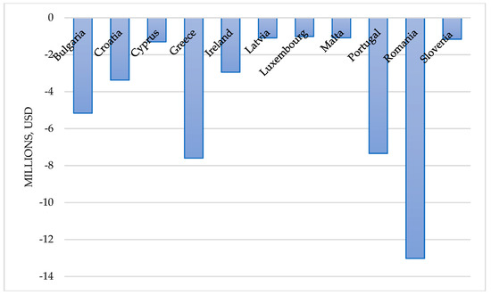
Figure 1.
The average export differences of the first group countries for 2014–2018, USD (designed by authors).
Only Denmark suffered export losses from the second groups of countries (Figure 2). The actual exports of Austria, Czech Republic, Estonia, Hungary, Lithuania, Slovak Republic, Spain, and Sweden, for 2014–2018, were higher than expected, and the embargo had no negative impact on the export of products to Russia. According to the gravitational equation, Lithuania’s export forecast for 2014–2018 was lower than actual exports. Thus, Lithuania did not suffer export losses. Although Lithuania has almost stopped exporting some of its products to Russia, the embargo did not have a negative impact on the entire export of Lithuanian products.
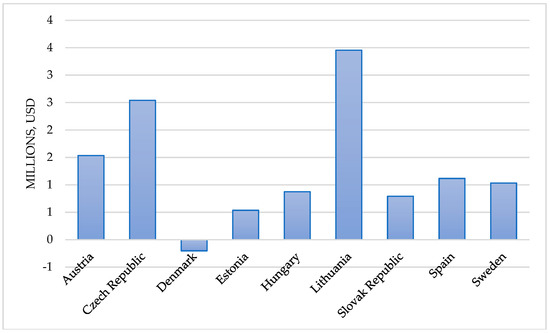
Figure 2.
The average export differences of the second group countries for 2014–2018, USD (designed by authors).
The actual exports of Belgium, Finland, France, Italy, Netherlands, Poland, United Kingdom, and Germany, for 2014–2018, were higher than expected, and the embargo had no negative impact on the export of products to Russia (Figure 3). The difference in Germany is the biggest because, before the embargo, Germany’s export to Russia was considerable and, after the embargo, Germany suffered significant losses, which explains why its forecast export is small. Although Germany lost a lot, it recovered quite fast, it started to export different production to Russia, and that is why its actual export remained large.
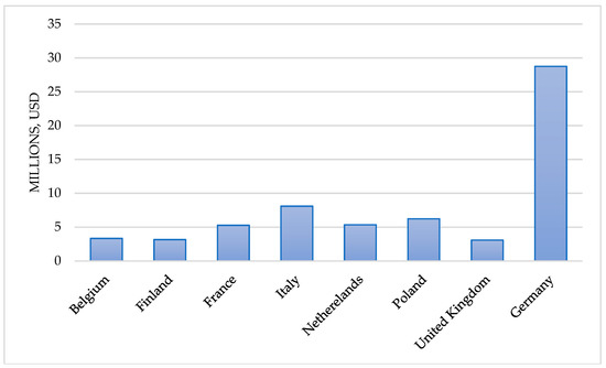
Figure 3.
The average of export differences of the third and fourth group countries for 2014–2018, USD (made by author).
According to the European Union export variation for 2014–2018, the total loss of exports of products to Russia by all European Union countries amounted to USD 226,850 million.
It should be noted that the analysis of the export data of the products covered all the products. Therefore, these data cannot be understood as the loss caused only by the embargo of certain products announced by Russia. The embargo, of course, had the most significant impact on the decrease in exports of products to Russia, but other factors could have contributed to the decline in exports. Because none of the gravity models formed was 100% accurate, it can be concluded that the various factors not included in the gravity model also influenced the change in export volumes.
Taking into account the export losses of the European Union countries for 2014–2018, the most significant export losses were made by the countries that exported the least products to Russia, before the embargo was issued, because they did not try to find a solution. Countries that exported a lot before the embargo found a solution to recover. Most of them started to export different products for which the embargo was not imposed. Germany’s export difference between actual and forecasted values for 2014–2018 was the highest in all EU countries because it was the largest exporter to Russia and, after the embargo, it suffered significant losses, forecasted values fell, but Germany recovered quite fast. Austria, Czech Republic, Estonia, Hungary, Lithuania, Slovak Republic, Spain, Sweden, Belgium, Finland, France, Italy, Netherlands, Poland, United Kingdom, and Germany did not suffer significant losses because of the embargo. In summary, the Russian embargo on imports has not had a negative impact on almost all countries of the European Union looking through a long-time perspective.
5. Conclusions
After an analysis of the theoretical aspects of the influence of political decisions on a country’s economic relations, we conclude that economic relations and politics are strongly related. Economic relations can be analysed through economic indicators such as gross domestic product (GDP), imports, exports, foreign direct investments (FDI), and others. According to the scientific articles, political decisions can be divided into the following groups: agreements and memberships in organisations, embargos and sanctions, help for local businesses, and changes in domestic policy. Political decisions can have negative, positive or both negative and positive impacts. Moreover, political decisions can have an effect at a national, global or national and global level, and also an effect on the economy, society, or relations with other countries.
The analysis of international trade between the European Union and Russia requires an assessment of the significant gravity model factors. The gravity model helps to evaluate the impact of the embargo on EU exports and to make a prospective analysis. This model is used to analyse trade flows by selecting geographic, demographic, and economic variables of the model. The research consists of two parts. In the first part of the study, the correlation and regression analysis of the gravity equation is performed. In addition, the adjusted gravity equation is made, according to which the forecasts of the export volumes of each EU country to Russia for 2014–2018 are performed by using moving average and exponential smoothing methods. The projected export volumes are compared with the actual export volumes, and the impact of the embargo on each country’s exports is assessed. EU countries are divided into groups by using cluster analysis to evaluate the effect of the embargo on each country. In the second part of the research, according to the equation of the gravity model, forecasting of export of products of every EU country to Russia is made for 2019 by using the moving average method.
The theoretical values of European Union exports to Russia for 2014–2018 were calculated by using the gravity method and compared with the actual values. It is estimated that the most significant export losses were made for the countries that exported the least number of products to Russia before the embargo was issued. Germany’s export difference between actual and forecasted values for 2014–2018 was the highest in all EU countries because it was the largest exporter to Russia. After the embargo, it suffered significant losses, forecasts fell, but Germany recovered quite fast. Austria, Czech Republic, Estonia, Hungary, Lithuania, Slovak Republic, Spain, Sweden, Belgium, Finland, France, Italy, Netherlands, Poland, United Kingdom, and Germany did not suffer significant losses due to the embargo.
The results of the study could be useful for the EU countries public authorities that want to investigate the current state or predict future export volumes.
The current study has several limitations. The research reflects only the impact of the embargo on exports, while other factors may also affect export volumes. Moreover, due to the lack of data, the study assesses the export of all sectors.
6. Future Research Directions
To evaluate embargo impact more precisely other factors that could affect export volume should be assessed. Moreover, in future research, different export sectors could be evaluated separately, and analysis of the effect of a different factor on each industry could be conducted.
Author Contributions
Conceptualisation, VS and SV; methodology, VS and SV; software, VS and SV; validation, V.S., S.V. and D.J.; formal analysis, V.S., S.V. and D.J.; investigation, V.S., S.V. and D.J.; resources, V.S., S.V. and D.J.; data curation, V.S. and S.V.; writing, V.S., S.V. and D.J.. All authors have read and agreed to the published version of the manuscript.
Funding
This research received no external funding.
Conflicts of Interest
The authors declare no conflict of interest.
Appendix A

Figure A1.
Dendrogram.
Appendix B
Table A1.
Comparison of estimated predicted values with actual values of European Union countries’ export to Russia.
Table A1.
Comparison of estimated predicted values with actual values of European Union countries’ export to Russia.
| Country | Year | Forecasted Values by Moving Average Method | Forecasted Values by Exponential Smoothing Method | ||||
|---|---|---|---|---|---|---|---|
| FEUGDP | FRUGDP | Fpop | FEUGDP | FRUGDP | Fpop | ||
| Austria | 2014 | 321,734.1 | 1,068,511 | 8,203,226 | 218,557.00 | 290,231.00 | 8,415,917.06 |
| 2015 | 328,849.6 | 1,126,632 | 8,221,141 | 218,557.00 | 290,231.00 | 8,461,851.53 | |
| 2016 | 331,802.3 | 1,139,803 | 8,241,352 | 218,557.00 | 290,231.00 | 8,523,388.76 | |
| 2017 | 335,087.2 | 1,147,322 | 8,265,516 | 218,557.00 | 290,231.00 | 8,611,929.88 | |
| 2018 | 339,216.5 | 1,168,877 | 8,290,883 | 218,557.00 | 290,231.00 | 8,692,397.44 | |
| Belgium | 2014 | 391,076.3 | 1,068,511 | 10,561,664 | 260,952.00 | 290,231.00 | 1,1057,617.29 |
| 2015 | 399,345.4 | 1,126,632 | 10,598,086 | 260,952.00 | 290,231.00 | 1,1119,228.65 | |
| 2016 | 402,496.6 | 1,139,803 | 10,633,597 | 260,952.00 | 290,231.00 | 1,1178,251.32 | |
| 2017 | 406,045.7 | 1,147,322 | 10,669,256 | 260,952.00 | 290,231.00 | 1,1244,684.16 | |
| 2018 | 410,531.3 | 1,168,877 | 10,703,379 | 260,952.00 | 290,231.00 | 1,1298,205.58 | |
| Bulgaria | 2014 | 34,320.94 | 1,068,511 | 7,722,006 | 13,227.00 | 290,231.00 | 7,329,212.68 |
| 2015 | 35,644.12 | 1,126,632 | 7,693,987 | 13,227.00 | 290,231.00 | 7,287,444.84 | |
| 2016 | 36,452.83 | 1,139,803 | 7,666,665 | 13,227.00 | 290,231.00 | 7,244,821.42 | |
| 2017 | 37,336.16 | 1,147,322 | 7,639,671 | 13,227.00 | 290,231.00 | 7,199,302.71 | |
| 2018 | 38,386.1 | 1,168,877 | 7,612,781 | 13,227.00 | 290,231.00 | 7,150,580.85 | |
| Croatia | 2014 | 45,177.25 | 1,068,511 | 4,341,468 | 25,346.00 | 290,231.00 | 4,274,680.10 |
| 2015 | 45,912.88 | 1,126,632 | 4,335,900 | 25,346.00 | 290,231.00 | 4,260,744.55 | |
| 2016 | 46,113.22 | 1,139,803 | 4,329,756 | 25,346.00 | 290,231.00 | 4,243,030.28 | |
| 2017 | 46,403.21 | 1,147,322 | 4,322,436 | 25,346.00 | 290,231.00 | 4,216,849.64 | |
| 2018 | 46,843.1 | 1,168,877 | 4,314,025 | 25,346.00 | 290,231.00 | 4,185,531.32 | |
| Cyprus | 2014 | 18,990.5 | 1,068,511 | 755,207.1 | 10,251.00 | 290,231.00 | 853,295.87 |
| 2015 | 19,249.94 | 1,126,632 | 761,253.8 | 10,251.00 | 290,231.00 | 855,647.93 | |
| 2016 | 19,274.44 | 1,139,803 | 766,017.9 | 10,251.00 | 290,231.00 | 851,327.97 | |
| 2017 | 19,336.89 | 1,147,322 | 770,349.5 | 10,251.00 | 290,231.00 | 849,823.48 | |
| 2018 | 19,479.35 | 1,168,877 | 774,572.2 | 10,251.00 | 290,231.00 | 852,312.74 | |
| Czech Republic | 2014 | 146,033.7 | 1,068,511 | 10,319,019 | 66,465.00 | 290,231.00 | 1,0496,462.46 |
| 2015 | 149,668.1 | 1,126,632 | 10,330,396 | 66,465.00 | 290,231.00 | 1,0504,440.73 | |
| 2016 | 151,732.6 | 1,139,803 | 10,341,945 | 66,465.00 | 290,231.00 | 1,0521,357.87 | |
| 2017 | 154,014.6 | 1,147,322 | 10,353,097 | 66,465.00 | 290,231.00 | 1,0537,600.43 | |
| 2018 | 157,109.6 | 1,168,877 | 10,364,383 | 66,465.00 | 290,231.00 | 1,0558,210.22 | |
| Denmark | 2014 | 263,132.6 | 1,068,511 | 5,436,804 | 176,991.00 | 290,231.00 | 5,580,072.68 |
| 2015 | 268,418.5 | 1,126,632 | 5,448,006 | 176,991.00 | 290,231.00 | 5,603,653.84 | |
| 2016 | 270,321.6 | 1,139,803 | 5,459,768 | 176,991.00 | 290,231.00 | 5,631,684.42 | |
| 2017 | 272,514.5 | 1,147,322 | 5,472,793 | 176,991.00 | 290,231.00 | 5,669,467.71 | |
| 2018 | 275,382.1 | 1,168,877 | 5,486,592 | 176,991.00 | 290,231.00 | 5,709,118.36 | |
| Estonia | 2014 | 15,049.75 | 1,068,511 | 1,357,889 | 5,621.00 | 290,231.00 | 1,324,689.73 |
| 2015 | 15,732.59 | 1,126,632 | 1,355,414 | 5,621.00 | 290,231.00 | 1,320,254.37 | |
| 2016 | 16,131.67 | 1,139,803 | 1,353,162 | 5,621.00 | 290,231.00 | 1,317,562.18 | |
| 2017 | 16,545.47 | 1,147,322 | 1,351,203 | 5,621.00 | 290,231.00 | 1,316,753.09 | |
| 2018 | 17,051.45 | 1,168,877 | 1,349,425 | 5,621.00 | 290,231.00 | 1,316,194.05 | |
| Finland | 2014 | 206,038.7 | 1,068,511 | 5,264,433 | 134,110.00 | 290,231.00 | 5,401,448.84 |
| 2015 | 209,980.1 | 1,126,632 | 5,275,423 | 134,110.00 | 290,231.00 | 5,426,359.42 | |
| 2016 | 211,235.7 | 1,139,803 | 5,286,331 | 134,110.00 | 290,231.00 | 5,449,056.21 | |
| 2017 | 212,704.9 | 1,147,322 | 5,296,908 | 134,110.00 | 290,231.00 | 5,468,182.11 | |
| 2018 | 214,710.1 | 1,168,877 | 5,307,228 | 134,110.00 | 290,231.00 | 5,485,739.55 | |
| France | 2014 | 2,188,928 | 1,068,511 | 62,857,376 | 1,505,184.00 | 290,231.00 | 6,5281,656.96 |
| 2015 | 2,228,209 | 1,126,632 | 63,038,840 | 1,505,184.00 | 290,231.00 | 6,5611,961.98 | |
| 2016 | 2,239,944 | 1,139,803 | 63,228,698 | 1,505,184.00 | 290,231.00 | 6,6034,120.49 | |
| 2017 | 2,251,849 | 1,147,322 | 63,413,001 | 1,505,184.00 | 290,231.00 | 6,6382,286.75 | |
| 2018 | 2,268,641 | 1,168,877 | 63,591,805 | 1,505,184.00 | 290,231.00 | 6,6685,684.87 | |
| Germany | 2014 | 2,923,185 | 1,068,511 | 81,898,499 | 2,246,306.00 | 290,231.00 | 8,0618,807.16 |
| 2015 | 2,980,934 | 1,126,632 | 81,831,967 | 2,246,306.00 | 290,231.00 | 8,0693,135.08 | |
| 2016 | 3,003,276 | 1,139,803 | 81,796,721 | 2,246,306.00 | 290,231.00 | 8,0945,336.04 | |
| 2017 | 3,029,241 | 1,147,322 | 81,816,666 | 2,246,306.00 | 290,231.00 | 8,1560,510.02 | |
| 2018 | 3,062,810 | 1,168,877 | 81,851,916 | 2,246,306.00 | 290,231.00 | 8,2041,081.51 | |
| Greece | 2014 | 235,079.0 | 1,068,511 | 10,956,004 | 144,644.00 | 290,231.00 | 1,1050,265.04 |
| 2015 | 235,215.9 | 1,126,632 | 10,954,287 | 144,644.00 | 290,231.00 | 1,0988,536.02 | |
| 2016 | 233,075.6 | 1,139,803 | 10,948,938 | 144,644.00 | 290,231.00 | 1,0923,277.01 | |
| 2017 | 231,087.5 | 1,147,322 | 10,940,244 | 144,644.00 | 290,231.00 | 1,0853,512.51 | |
| 2018 | 229,707.8 | 1,168,877 | 10,931,642 | 144,644.00 | 290,231.00 | 1,0810,852.75 | |
| Hungary | 2014 | 102,983.6 | 1,068,511 | 10,096,655 | 48,770.00 | 290,231.00 | 9,939,455.09 |
| 2015 | 105,165.9 | 1,126,632 | 10,083,755 | 48,770.00 | 290,231.00 | 9,908,410.05 | |
| 2016 | 106,160.8 | 1,139,803 | 10,071,078 | 48,770.00 | 290,231.00 | 9,881,990.52 | |
| 2017 | 107,205.4 | 1,147,322 | 10,058,415 | 48,770.00 | 290,231.00 | 9,856,237.76 | |
| 2018 | 108,833.2 | 1,168,877 | 10,045,373 | 48,770.00 | 290,231.00 | 9,826,899.38 | |
| Ireland | 2014 | 13,464.63 | 1,068,511 | 4,180,431 | 8,494.00 | 290,231.00 | 4,584,977.59 |
| 2015 | 13,717.18 | 1,126,632 | 4,207,338 | 8,494.00 | 290,231.00 | 4,611,414.79 | |
| 2016 | 13,921.17 | 1,139,803 | 4,233,465 | 8,494.00 | 290,231.00 | 4,644,520.90 | |
| 2017 | 14,273.63 | 1,147,322 | 4,259,403 | 8,494.00 | 290,231.00 | 4,685,403.45 | |
| 2018 | 14,784.60 | 1,168,877 | 4,285,652 | 8,494.00 | 290,231.00 | 4,734,893.22 | |
| Italy | 2014 | 1,792,526 | 1,068,511 | 58,047,629 | 1,267,952.00 | 290,231.00 | 5,9477,935.80 |
| 2015 | 1,813,857 | 1,126,632 | 58,208,513 | 1,267,952.00 | 290,231.00 | 6,0130,301.90 | |
| 2016 | 1,814,931 | 1,139,803 | 58,352,241 | 1,267,952.00 | 290,231.00 | 6,0462,956.95 | |
| 2017 | 1,817,828 | 1,147,322 | 58,473,994 | 1,267,952.00 | 290,231.00 | 6,0564,253.98 | |
| 2018 | 1,824,281 | 1,168,877 | 58,579,767 | 1,267,952.00 | 290,231.00 | 6,0576,849.49 | |
| Latvia | 2014 | 19,297.19 | 1,068,511 | 2,234,802 | 7,178.00 | 290,231.00 | 2,051,653.95 |
| 2015 | 20,008.24 | 1,126,632 | 2,221,076 | 7,178.00 | 290,231.00 | 2,026,560.98 | |
| 2016 | 20,395.89 | 1,139,803 | 2,208,022 | 7,178.00 | 290,231.00 | 2,006,328.49 | |
| 2017 | 20,780.68 | 1,147,322 | 2,195,440 | 7,178.00 | 290,231.00 | 1,987,642.74 | |
| 2018 | 21,267.85 | 1,168,877 | 2,183,173 | 7,178.00 | 290,231.00 | 1,968,879.37 | |
| Lithuania | 2014 | 28,354.19 | 1,068,511 | 3,302,775 | 11,241.00 | 290,231.00 | 3,015,991.65 |
| 2015 | 29,547.00 | 1,126,632 | 3,281,640 | 11,241.00 | 290,231.00 | 2,979,731.82 | |
| 2016 | 30,213.17 | 1,139,803 | 3,261,619 | 11,241.00 | 290,231.00 | 2,950,496.91 | |
| 2017 | 30,885.68 | 1,147,322 | 3,241,984 | 11,241.00 | 290,231.00 | 2,919,527.46 | |
| 2018 | 31,723.40 | 1,168,877 | 3,222,280 | 11,241.00 | 290,231.00 | 2,883,715.73 | |
| Luxembourg | 2014 | 40,088.38 | 1,068,511 | 470,556.9 | 19,341.00 | 290,231.00 | 525,404.11 |
| 2015 | 41,624.88 | 1,126,632 | 475,211.2 | 19,341.00 | 290,231.00 | 537,542.05 | |
| 2016 | 42,492.00 | 1,139,803 | 480.086 | 19,341.00 | 290,231.00 | 550,250.03 | |
| 2017 | 43,360.05 | 1,147,322 | 485,147.2 | 19,341.00 | 290,231.00 | 563,249.51 | |
| 2018 | 44,314.10 | 1,168,877 | 490,423.2 | 19,341.00 | 290,231.00 | 576,958.26 | |
| Malta | 2014 | 6746.19 | 1,068,511 | 402,728.9 | 3,682.00 | 290,231.00 | 418,918.35 |
| 2015 | 7014.18 | 1,126,632 | 404,299.2 | 3,682.00 | 290,231.00 | 424,171.17 | |
| 2016 | 7219.00 | 1,139,803 | 406,265.4 | 3,682.00 | 290,231.00 | 431,931.09 | |
| 2017 | 7441.47 | 1,147,322 | 408,589.1 | 3,682.00 | 290,231.00 | 441,173.04 | |
| 2018 | 7707.10 | 1,168,877 | 411,174.5 | 3,682.00 | 290,231.00 | 450,735.02 | |
| Netherlands | 2014 | 687,947.3 | 1,068,511 | 16,278,185 | 438,610.00 | 290,231.00 | 1,6716,844.41 |
| 2015 | 699,973.8 | 1,126,632 | 16,310,603 | 438,610.00 | 290,231.00 | 1,6773,066.70 | |
| 2016 | 703,622.4 | 1,139,803 | 16,343,387 | 438,610.00 | 290,231.00 | 1,6836,896.35 | |
| 2017 | 707,845.1 | 1,147,322 | 16,376,847 | 438,610.00 | 290,231.00 | 1,6908,008.18 | |
| 2018 | 714,064.8 | 1,168,877 | 16,412,080 | 438,610.00 | 290,231.00 | 1,6994,757.59 | |
| Poland | 2014 | 341,270.4 | 1,068,511 | 38,213,460 | 172,050.00 | 290,231.00 | 3,8064,910.44 |
| 2015 | 353,271.2 | 1,126,632 | 38,201,954 | 172,050.00 | 290,231.00 | 3,8041,383.22 | |
| 2016 | 360,176.6 | 1,139,803 | 38,191,046 | 172,050.00 | 290,231.00 | 3,8023,498.61 | |
| 2017 | 366,053.7 | 1,147,322 | 38,179,265 | 172,050.00 | 290,231.00 | 3,7995,353.81 | |
| 2018 | 374,080.8 | 1,168,877 | 38,168,950 | 172,050.00 | 290,231.00 | 3,7984,158.90 | |
| Portugal | 2014 | 191,397.3 | 1,068,511 | 10,440,249 | 124,159.00 | 290,231.00 | 1,0520,884.38 |
| 2015 | 193,667.8 | 1,126,632 | 10,439,488 | 124,159.00 | 290,231.00 | 1,0474,092.69 | |
| 2016 | 193,992.9 | 1,139,803 | 10,435,895 | 124,159.00 | 290,231.00 | 1,0424,457.35 | |
| 2017 | 194,643.9 | 1,147,322 | 10,430,918 | 124,159.00 | 290,231.00 | 1,0382,893.67 | |
| 2018 | 195,899.1 | 1,168,877 | 10,424,851 | 124,159.00 | 290,231.00 | 1,0346,233.34 | |
| Romania | 2014 | 114,843.3 | 1,068,511 | 21,271,137 | 42,815.00 | 290,231.00 | 2,0120,793.76 |
| 2015 | 119,830.6 | 1,126,632 | 21,193,265 | 42,815.00 | 290,231.00 | 2,0034,052.38 | |
| 2016 | 123,056.4 | 1,139,803 | 21,119,787 | 42,815.00 | 290,231.00 | 1,9952,349.69 | |
| 2017 | 126,500.6 | 1,147,322 | 21,048,235 | 42,815.00 | 290,231.00 | 1,9856,331.85 | |
| 2018 | 130,745.9 | 1,168,877 | 20,978,041 | 42,815.00 | 290,231.00 | 1,9750,340.92 | |
| Slovak Republic | 2014 | 58,586.94 | 1,068,511 | 5,384,965 | 22,804.00 | 290,231.00 | 5,403,614.15 |
| 2015 | 61,088.24 | 1,126,632 | 5,386,788 | 22,804.00 | 290,231.00 | 5,409,781.58 | |
| 2016 | 62,573.00 | 1,139,803 | 5,388,708 | 22,804.00 | 290,231.00 | 5,415,565.29 | |
| 2017 | 64,010.47 | 1,147,322 | 5,390,684 | 22,804.00 | 290,231.00 | 5,420,908.64 | |
| 2018 | 65,600.4 | 1,168,877 | 5,392,917 | 22,804.00 | 290,231.00 | 5,428,125.82 | |
| Slovenia | 2014 | 37,403.63 | 1,068,511 | 2,012,002 | 22,147.00 | 290,231.00 | 2,053,744.93 |
| 2015 | 38,142.76 | 1,126,632 | 2,014,889 | 22,147.00 | 290,231.00 | 2,057,414.96 | |
| 2016 | 38,419.5 | 1,139,803 | 2,017,555 | 22,147.00 | 290,231.00 | 2,060,144.48 | |
| 2017 | 38,747.95 | 1,147,322 | 2,020,010 | 22,147.00 | 290,231.00 | 2,062,166.24 | |
| 2018 | 39,238.2 | 1,168,877 | 2,022,304 | 22,147.00 | 290,231.00 | 2,064,030.62 | |
| Spain | 2014 | 1,114,730 | 1,068,511 | 43,605,775 | 616,885.00 | 290,231.00 | 4,6654,103.53 |
| 2015 | 1,130,281 | 1,126,632 | 43,776,741 | 616,885.00 | 290,231.00 | 4,6583,151.27 | |
| 2016 | 1,134,137 | 1,139,803 | 43,925,231 | 616,885.00 | 290,231.00 | 4,6516,358.13 | |
| 2017 | 1,139,604 | 1,147,322 | 44,057,593 | 616,885.00 | 290,231.00 | 4,6478,228.57 | |
| 2018 | 1,148,471 | 1,168,877 | 44,181,065 | 616,885.00 | 290,231.00 | 4,6502,633.78 | |
| Sweden | 2014 | 402,284.1 | 1,068,511 | 9,104,902 | 267,225.00 | 290,231.00 | 9,483,755.09 |
| 2015 | 412,409.3 | 1,126,632 | 9,136,664 | 267,225.00 | 290,231.00 | 9,564,309.54 | |
| 2016 | 417,170.9 | 1,139,803 | 9,170,591 | 267,225.00 | 290,231.00 | 9,655,832.27 | |
| 2017 | 422,172.7 | 1,147,322 | 9,206,403 | 267,225.00 | 290,231.00 | 9,753,424.64 | |
| 2018 | 427,844.4 | 1,168,877 | 9,245,841 | 267,225.00 | 290,231.00 | 9,874,288.82 | |
| United Kingdom | 2014 | 2,311,879 | 1,068,511 | 60,732,315 | 1,641,822.00 | 290,231.00 | 6,3459,803.01 |
| 2015 | 2,354,493 | 1,126,632 | 60,945,188 | 1,641,822.00 | 290,231.00 | 6,3905,479.01 | |
| 2016 | 2,384,635 | 1,139,803 | 61,163,520 | 1,641,822.00 | 290,231.00 | 6,4390,322.00 | |
| 2017 | 2,399,608 | 1,147,322 | 61,385,574 | 1,641,822.00 | 290,231.00 | 6,4886,439.00 | |
| 2018 | 2,411,626 | 1,168,877 | 61,606,724 | 1,641,822.00 | 290,231.00 | 6,5347,506.00 | |
References
- Ahad, Nor Aishah, Teh Sin Yin, Abdul Rahman Othman, and Che Rohani Yaacob. 2011. Sensitivity of normality tests to non-normal data (kepekaan ujian kenormalan terhadap data tidak normal). Sains Malaysiana 40: 637–41. [Google Scholar]
- Anderson, James E. 2011. The gravity model. Annual Review of Economics 3: 133–60. [Google Scholar] [CrossRef]
- Battaglini, Marco, and Stephen Coate. 2008. The political economy of fiscal policy. Journal of the European Economic Association 6: 367–80. [Google Scholar] [CrossRef]
- Bejan, Maria. 2011. Trade agreements and international comovements: The case of NAFTA (North American free trade agreement). Review of Economic Dynamics 14: 667–85. [Google Scholar] [CrossRef]
- Bhandari, Pranjul, and Jeffrey A. Frankel. 2017. Nominal GDP targeting for developing countries. Research in Economics 71: 491–506. [Google Scholar] [CrossRef]
- Castellani, Davide, and Claudio Fassio. 2019. From new imported inputs to new exported products. firm-level evidence from Sweden. Research Policy 48: 322–38. [Google Scholar] [CrossRef]
- Coudert, Virginie, Cécile Couharde, Carl Grekou, and Valérie Mignon. 2020. Heterogeneity within the euro area: New insights into an old story. Economic Modelling 90: 428–44. [Google Scholar] [CrossRef]
- Dou, Lei, Koji Yanagishima, Xin Li, Ping Li, and Mitsuhiro Nakagawa. 2015. Food safety regulation and its implication on chinese vegetable exports. Food Policy 5: 128–34. [Google Scholar] [CrossRef]
- Doumbe, Eric, and Thierry Belinga. 2015. A gravity model analysis for trade between cameroon and twenty-eight european union countries. Open Journal of Social Sciences 3: 114–222. [Google Scholar] [CrossRef]
- Fetahu, Elvira. 2014. Trade integration between albania and european union a gravity model based analysis. European Scientific Journal (ESJ) 10. [Google Scholar] [CrossRef]
- García Costa, Beatriz, Laura García Costa, and Raúl Gómez Martínez. 2019. Does political uncertainty affect investment in ibex 35?’. Cuadernos de Economía—Spain 42: 163–74. [Google Scholar] [CrossRef]
- Ge, Yongbo, Tingting Cao, Ruchuan Jiang, Peide Liu, and Hengxin Xie. 2019. Does China’s iron ore futures market have price discovery function? Analysis based on VECM and state-space perspective. Journal of Business Economics and Management 20: 1083–101. [Google Scholar] [CrossRef]
- Gharehgozli, Orkideh. 2017. An estimation of the economic cost of recent sanctions on iran using the synthetic control method. Economics Letters 157: 141–44. [Google Scholar] [CrossRef]
- Gil-González, Diana, Mercedes Carrasco-Portiño, Ma Carmen Davó Blanes, Lucas Donat Castelló, Álvaro Franco-Giraldo, Rocio Ortiz Moncada, Marco Palma Solís, and et al. 2008. Appraissal of the millennium development goals by means of a review of the scientific literature in 2008′. Revista Espanola de Salud Publica 82: 455–66. [Google Scholar] [PubMed]
- Gurvich, Evsey, and Ilya Prilepskiy. 2015. The impact of financial sanctions on the russian economy. Russian Journal of Economics 1: 359–85. [Google Scholar] [CrossRef]
- Hodder, Jake. 2017. White world order, black power politics: The birth of american international relations. Journal of Historical Geography 56: 155–56. [Google Scholar] [CrossRef]
- Hübner, Kurt. 2016. CETA: The Making of the Comprehensive Economic and Trade Agreement Between Canada and the EU. Available online: http://trade.ec.europa.eu/doclib/docs/2014/september/tradoc_152806.pdf (accessed on 9 May 2020).
- Imbruno, Michele. 2016. China and WTO Liberalisation: Imports, tariffs and non-tariff barriers. China Economic Review 38: 222–37. [Google Scholar] [CrossRef]
- Januškevičius, Andrius. 2017. Euro Įvedimas Lietuvai Atnešė Daugiau Naudos Nei Neigiamų Aspektų. Available online: http://bit.ly/2lF7lcO (accessed on 2 April 2020).
- Knox, Eleanor. 2011. Newton–Cartan theory and teleparallel gravity: The force of a formulation. Studies in History and Philosophy of Science Part B: Studies in History and Philosophy of Modern Physics 42: 264–75. [Google Scholar] [CrossRef]
- Maxim, Laura, and Jeroen P. van der Sluijs. 2011. Quality in environmental science for policy: Assessing uncertainty as a component of policy analysis. Environmental Science & Policy 14: 482–92. [Google Scholar] [CrossRef]
- Mellor, John W. 1964. Tinbergen, Jan, Shaping the world economy: Suggestions for an international economic policy, New York, the twentieth century fund, 1962, Pp. Xviii, 330. (Cloth, $4.00; Paper, $2.25). American Journal of Agricultural Economics 46: 271–73. [Google Scholar] [CrossRef]
- Mitra, Devashish, and Jeongeun Shin. 2012. Import protection, exports and labor-demand elasticities: Evidence from Korea. International Review of Economics & Finance 23: 91–109. [Google Scholar] [CrossRef]
- Monticelli, Jefferson Marlon, Cyntia Vilasboas Calixto, Silvio Luís Vasconcellos, and Ivan Lapuente Garrido. 2017. The influence of formal institutions on the internationalisation of companies in an emerging country. Review of Business Management 19: 358–74. [Google Scholar] [CrossRef]
- Nápoles, Pablo Ruiz. 2017. Neoliberal reforms and nafta in Mexico. Economía UNAM 14: 75–89. [Google Scholar] [CrossRef][Green Version]
- Neuenkirch, Matthias, and Florian Neumeier. 2015. The impact of UN and US economic sanctions on GDP growth. European Journal of Political Economy 40: 110–25. [Google Scholar] [CrossRef]
- Nguyen, Anh T. N. 2019. A global analysis of factors impacting the intensive and extensive margins of bilateral foreign direct investment. The World Economy, 1–19. [Google Scholar] [CrossRef]
- Official Statistic Portal. 2019. Main Lithuanian Indicators. Available online: https://osp.stat.gov.lt/pagrindiniai-salies-rodikliai (accessed on 2 February 2020).
- Orăştean, Ramona. 2013. Chinese currency internationalization—Present and expectations. Procedia Economics and Finance 6: 683–87. [Google Scholar] [CrossRef]
- Pinilla, Vicente, and Agustina Rayes. 2019. How argentina became a super-exporter of agricultural and food products during the first globalisation (1880–1929). Cliometrica 13: 443–69. [Google Scholar] [CrossRef]
- Razali, Nornadiah Mohd, and Yap Bee Wah. 2011. Power comparisons of shapiro-wilk, kolmogorov-smirnov, lilliefors and anderson-darling tests. Journal of Statistical Modeling and Analytics 2: 21–33. [Google Scholar]
- Riedel, Jana, and Anja Slany. 2019. The potential of african trade integration—Panel data evidence for the COMESA-EAC-SADC tripartite. The Journal of International Trade & Economic Development 28: 843–72. [Google Scholar] [CrossRef]
- Sasongko, Gatot, and Andrian Dolfriandra Huruta. 2018. Monetary policy and the causality between inflation and money supply in indonesia. Business: Theory and Practice 19: 80–87. [Google Scholar] [CrossRef]
- Schulte, Simon, and Florian Weiser. 2019. LNG import quotas in lithuania—Economic effects of breaking gazprom’s natural gas monopoly. Energy Economics 78: 174–81. [Google Scholar] [CrossRef]
- Shahriar, Saleh, Lu Qian, and Sokvibol Kea. 2019. Determinants of exports in China’s meat industry: A gravity model analysis. Emerging Markets Finance and Trade 55: 2544–65. [Google Scholar] [CrossRef]
- Shapiro, Samuel Sanford, and Martin Wilk. 1965. An analysis of variance test for normality (complete samples). Biometrika 52: 591. [Google Scholar] [CrossRef]
- Steinskog, Dag J., Dag B. Tjøstheim, and Nils G. Kvamstø. 2007. A cautionary note on the use of the kolmogorov–smirnov test for normality. Monthly Weather Review 135: 1151–57. [Google Scholar] [CrossRef]
- Stremousova, Elena, and Olga Buchinskaia. 2019. Some approaches to evaluation macroeconomic efficiency of digitalisation. Business, Management and Education 17: 232–47. [Google Scholar] [CrossRef]
- The Department of Statistics of the Republic of Lithuania. 2017. Legal Alcohol Consumption. Available online: http://osp.stat.gov.lt/statistiniu-rodikliu-analize?id=2034&status=A (accessed on 15 January 2019).
- Tkáčová, Andrea, Beáta Gavurová, and Viliam Kováč. 2018. Political-economic cycle models of economy of greece. Journal of Business Economics and Management 19: 742–58. [Google Scholar] [CrossRef]
- Venkuviene, Vitalija, and Ruta Masteikiene. 2015. The impact of russian federation economic embargo on the central and eastern european countries business environments. Procedia Economics and Finance 26: 1095–101. [Google Scholar] [CrossRef][Green Version]
- Wang, Kuang-Cheng A, Hui-Wen Koo, and Tain-Jy Chen. 2011. Domestic trade protection in vertically-related markets. Economic Modelling 28: 1595–603. [Google Scholar] [CrossRef]
- Wang, Mingyue, and Rui Kong. 2019. Study on the characteristics of potassium salt international trade based on complex network. Journal of Business Economics and Management 20: 1000–21. [Google Scholar] [CrossRef]
- Witkowska, Dorota, Krzysztof Kompa, and Grzegorz Mentel. 2019. The effect of government decisions on the efficiency of the invetment funds market in Poland. Journal of Business Economics and Management 20: 573–94. [Google Scholar] [CrossRef]
- Yang, Yong-cong, and Pu-yan Nie. 2020. Optimal trade policies under product differentiations. Journal of Business Economics and Management 21: 241–54. [Google Scholar] [CrossRef]
© 2020 by the authors. Licensee MDPI, Basel, Switzerland. This article is an open access article distributed under the terms and conditions of the Creative Commons Attribution (CC BY) license (http://creativecommons.org/licenses/by/4.0/).