Abstract
This study empirically investigates the relationship between economic growth and several factors (investment, private and government consumption, trade openness, population growth and government debt) in Greece, where imbalances persist several years after the financial crisis. The results reveal a long-run relationship between variables. Investment as private and government consumption and trade openness affect positively growth. On the other hand, there is a negative long-run effect of government debt and population growth on growth. Furthermore, the study addresses the issue of break effects between government debt and economic growth. The results indicate that the relationship between debt and growth depends on the debt breaks. Specifically, at debt levels before 2000, increases in the government debt-to-GDP ratio are associated with insignificant effects on economic growth. However, as government debt rises after 2000, the effect on economic growth diminishes rapidly and the growth impacts become negative. The challenge for policy makers in Greece is to halt the rising of government debt by keeping a sustainable growth path. Fiscal discipline should be combined with the implementation of coherent, consistent and sequential growth-enhancing structural reforms.
JEL Classification:
C24; C32; H63; O11; O40
1. Introduction
The rising government debt levels and its interactions with other determinants of economic growth, especially in the aftermath of global financial crisis, have necessitated the revival of the academic and policy debate on the impact of growing debt levels on growth (Jiménez-Rodríguez and Rodríguez-López 2015; Bökemeier and Greiner 2015; Swamy 2015a, 2015b). In advanced economies, government debt has been increased close to 50 percentage points since the start of the global financial crisis (International Monetary Fund 2016). Many countries in the Eurozone (especially peripheral countries) are struggling with a combination of high levels of indebtedness, budget deficits and frail growth.
The Greek crisis after the outbreak of the global financial crisis has occupied a central role in the public debates around the world. Greece, having longitudinal underlying pathologies, faced serious economic problems (fiscal, financial, structural, imbalances etc.). These problems have influenced other determinants of economic growth such as investment, consumption, trade openness and population growth. As a result, high levels of government debt made Greece the “weak link” of the economic crisis in the Eurozone. For that reason, Greece entered into economic adjustment programs and followed economic austerity policies. Greece entered the crisis of 2008 with the highest debt-to-GDP ratio among the economies of the Eurozone and had, together with Italy, the highest level of tax evasion and the biggest shadow economy within the EMU (Schneider 2011). Also, the Greek government deficit ratio increased rapidly from −6.7% of GDP in 2007 to −15.1% of GDP in 2009, while the debt-to-GDP ratio surged from 103 to 126.7% of GDP. Furthermore, rigidities in Greece’s product and labor markets have increased the cost of adjustment to large pre-crisis economic imbalances. Unit labor costs have increased far more in Greece than in all other EMU countries and under fixed exchange rates, this erodes competitiveness (International Monetary Fund 2013a, 2013b). Generally, in Greece during recent decades, some structural reforms and adjustments were implemented, more or less successfully. However, the Greek economy passed into the 21st century facing a number of unsolved problems, mainly high government deficit and debt.
The purpose of this study is to investigate the impact of government debt and other economic determinants (investment, private and public consumption, trade openness and population growth) on the growth of the Greek economy, by using the Autoregressive Distributed Lag (ARDL) model and the Vector Autoregressive Model (VAR) methodology. Also, this study explores the critical turning point at which the excessive government debt levels have a positive or negative impact on economic growth by using multiple structural break effects. It applies the methodology of Bai and Perron (1998, 2003) and the results reveal some evidence in favor of a negative relationship between debt and growth in Greece. The study compares the results from a linear macroeconomic model and a multiple structural break model, including the period of financial crisis. Thus, the results provide a comparison for the Greek economy, which may improve decision-making by policy makers.
The rest of the paper is organized as follows. Section 2 reviews the empirical literature. Section 3 presents the empirical analysis, explains methodology and presents sources and data. Section 4 presents the econometric analysis and reports and discusses the empirical results based on econometric analysis. Section 5 presents the concluding remarks and policy implication.
Review of Empirical Literature
Many studies of the empirical literature, especially after the financial crisis, focus on the impact of public debt on economic growth. First, the studies that have investigated the case of many countries by using cross-sectional data or panel data in their econometric analysis are presented. The basic findings from the empirical studies can be summarized as follows:
Pattillo et al. (2004) investigated whether debt affects growth for 61 developing countries over the period 1996–1998. The result showed that the negative impact of high debt on growth operates through a strong negative effect on physical capital accumulation and on growth. They also found positive effects of investment on economic growth. Schclarek (2004), focusing on a panel of 59 developing and 24 advanced countries over the period 1970–2002, concludes that, for developing countries, there is a negative relation between debt and growth, but he does not find any significant relation between government debt and economic growth in advanced countries. Also, the results show that investments and exports have a positive contribution to GDP growth. Sen et al. (2007) studied the impact of debt on economic growth of Argentina, Brazil, Columbia, Venezuela, Mexico, China, India, Indonesia, Philippines, Korea and Thailand. They came to the conclusion that debt negatively affects economic growth in Latin American and Asian countries. Misztal (2010), for a sample of EU Member States over the period 2000–2010, concluded that an increase in public debt by 1% in these countries has led, on average, to a reduction in GDP by 0.3%, while a GDP growth by 1% resulted in a reduction of public debt, on average, by 0.4%. Kumar and Woo (2010), for a panel of 38 developed and emerging countries over the period 1970–2007, found that a 10% increase of public debt is associated with a 0.2% decrease of GDP growth, the impact being stronger in emerging market economies and weaker in developed ones. Drine and Nabi (2010) for a panel of 27 developing countries for the period of 1970–2005 found that an increase in external public debt reduces production efficiency. Also, the results indicate that output is positively responsive to investment. Afonso and Jalles (2013) use a panel of 155 countries to assess the links between growth, productivity and government debt. They found a negative effect of the debt-to-GDP to economic growth and that financial crisis is detrimental for growth, while fiscal consolidation promotes growth. Afonso and Alves (2015) use a panel of 14 European countries to assess the links between growth, productivity and government debt. They found a negative effect of the debt-to-GDP to economic growth −0.04 and −0.03 and that financial crisis is detrimental for growth, while fiscal consolidation promotes growth.
Also, the literature includes studies that have investigated the case of one country by using time series data in their econometric analysis. Anyanwu and Erhijakpor (2004) studied the impact of debt on economic growth of Nigeria over the period 1970–2003. The study reported that debt has a significant negative impact on economic growth. El-Mahdy and Torayeh (2009) investigated the debt and growth relationship for Egypt’s economy using data spanning 1981–2006 and the study revealed a robust negative relationship between debt and growth. Ogunmuyiwa (2011) evaluated the effect of debt on Nigeria’s economic growth from 1970–2007. The results revealed a weak and insignificant relationship between debt and growth. Shah and Shahida (2012) investigated the effect of the public debt on economic growth of Bangladesh for the period 1980–2012 and found no impact of debt on economic growth. Tchereni et al. (2013) analyzed the effect of debt on Malawi’s economic growth over the period 1975–2003. They reported a statistically insignificant negative relationship between debt and economic growth in Malawi.
Also, some empirical studies sought to pin down and explain the relationship between public debt and growth, focusing on models with thresholds and breaks estimates. Cuestas et al. (2014) argue that government debt-to-GDP is likely to have a negative impact on the economic growth and also high levels of government debt are likely to have nonlinear effects on growth and that it becomes relevant only after a certain threshold value. Reinhart and Rogoff (2010) and Reinhart, Reinhart and Rogoff (Reinhart et al. 2012) argue that higher levels of government debt are negatively correlated with economic growth, but there is no link between debt and growth when government debt is below 90% of GDP. Supporting the study, other studies confirmed that the turning point beyond which growth gradually decreases is around 100% of GDP (Checherita-Westphal and Rother 2012; Furceri and Zdzienicka 2012). However, other studies could not identify a robust negative relationship between government debt and growth (Pescatori et al. 2014; Egert 2015; Eberhardt and Presbitero 2015).
The basic findings from the empirical studies can be summarized as follows: the majority of the studies have found a negative relationship between public debt and economic growth.
2. Empirical Analysis
2.1. Methodology
In our model, in order to determine the effect of debt-to-GDP ratio in GDP, we add on the right-hand side of equation some growth control variables, which include investment, private consumption, public consumption, trade openness and population growth. The first model specification as presented below assumes a linear relationship between debt-to-GDP and growth.
Y stands for real GDP in billion Euros, X is the GDP control variables (investment, private consumption, public consumption, trade openness and population growth). Debt represents the debt-to-GDP and εt is the error term.
Yt = α + βDebtt + γX’t + εt,
2.2. Sources and Data
Data on GDP, investment, private and government consumption, trade openness, population and debt-to-GDP are annual and were taken from AMECO database (AMECO 2017). GDP is measured at 2010 constant prices and investment is the gross fixed capital formation at 2010 constant prices. Private consumption is the private final consumption expenditure at 2010 prices. Government consumption is the final consumption expenditure of general government at 2010 prices. Trade openness is the sum of exports and imports of goods and services to GDP ratio, measured at 2010 constant prices. Debt-to-GDP is the ratio between Greece’s government debt and its GDP for the year.
Table 1 provides the descriptive statistics on the variables employed in the study. The data show that there are substantial variations for all variables over the examined period. Specifically, over the period 1970–2016, a significant GDP increase is observed. The average GDP in Greece was equal to 165 billion Euros and varies from 89 to 250. The average annual growth rate of GDP, over the whole period, was approximately 1.7% in real terms, but there were periods of very high growth rates (especially in the 1970s and 2000s) and periods of stagnation (particularly over the 2010–2016 period). The average debt-to-GDP is equal to 81. During the examined time period the debt-to-GDP has expanded rapidly. It increased from almost 16% in 1970, to 180% in 2016, exhibiting an average annual growth rate of 5.6%. The highest growth rate was during the 1980s and the lowest during the 2000s.The average investment is equal to 33 billion Euros and it varies from 21 to 62. The average annual growth rate of investment rate was 0.2% for the entire examined time period; with the highest growth rate seen during the 1990s and the lowest (negative) during the 1980s and the period 2010–2016.The average private consumption is equal to 105 and it varies from 47 to 171. Private consumption growth rate averaged 2.3% over the period 1970–2016. The highest growth rate occurred during the 1970s and the lowest (negative) during the period 2010–2016.The average government consumption is equal to 35 and it varies from 16 to 53. Government consumption increased by an average growth rate of 2.1% for the entire examined time period. The highest growth rate occurred during the 1970s and the lowest (negative) during the period 2010–2016. The average trade openness to GDP ratio is equal to 36 and it varies from 13 to 64. Trade openness experienced an average annual growth increase of 3.7% of GDP over the entire time period; with the highest growth rate seen during the 1970s and the lowest (negative) during the 2000s.The average population is equal to 10.244 million persons and it varies from 8.792 to 11.121. Population increased by an average annual growth of 0.4% over the period 1970–2016; with the highest growth rate seen during the 1970s and the lowest (negative) during the period 2010–2016.In order to compare the data, we concluded that in all the decades the GDP growth rate movements have been followed by similar movements in investment, private and government consumption, while debt-to-GDP growth rate were in the opposite direction. It is also worth mentioning that in the 2000s, when GDP had a significant positive growth rate, the trade openness had its lowest growth rate. On the other hand, during the period of economic stagnation (2010–2016) trade openness increased by an average annual growth of 3.4%.

Table 1.
Descriptive Statistics.
Moreover, Figure 1 and Figure 2 present the movement of debt and other determinants of the Greek economy over the period 1970–2016. Over the period 1995–2008, GDP has significantly increased, but after 2009 it rapidly decreased. The Greek economy has remained in recession during the period 2009–2016 and the recovery in 2014 was limited and soon fizzled out. With few exceptions for some years, investment, private and government consumption, trade openness and population have followed a similar course for the period 1970–2016. On the other hand debt-to-GDP has significantly increased over the period 1995–2008, but it rapidly increased during the period 2009–2016. Therefore, the graphs show that the economic crisis has a significant negative effect on economic growth as having been mentioned by the studies of Checherita-Westphal and Rother (2012) and Gómez-Puig and Sosvilla-Rivero (2015).
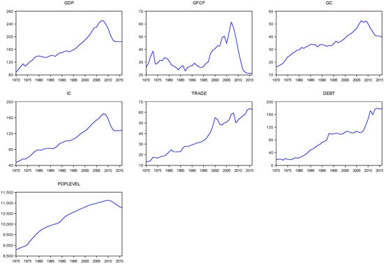
Figure 1.
Levels of the variables. (Source: The data selected from AMECO database for the time period 1970–2016. GDP is the real GDP, GFCF is the gross fixed capital formation, GC is the final consumption expenditure of general government, IC is the private final consumption expenditure. The amounts for these variables expressed in €billion. Debt is the debt-to-GDP ratio, trade is the trade openness-to-GDP ratio and pop is the population number in persons. All data are obtained from Authors’ calculations.).
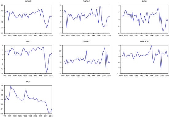
Figure 2.
Growth rates of the variables. (Source: The data selected from AMECO database for the time period 1970–2016. D indicates that the variables are expressed in growth rates. GDP is the real GDP, GFCF is the gross fixed capital formation, GC is the final consumption expenditure of general government, IC is the private final consumption expenditure, debt is the debt-to-GDP ratio, trade is the trade openness-to-GDP ratio and pop is the population number in persons. All data are obtained from Authors’ calculations.).
3. Econometric Analysis
This section focuses on the effect of government debt and investment, private consumption, public consumption, trade openness and population growth on economic growth, testing for cointegration so as to reveal any underlying long-run relationships among the variables. Then, we proceed with estimating a VAR model that reveals the impulse response functions and variance decomposition to investigate the dynamic relationships between the variables.
3.1. Unit Root Tests
Initially, the stationarity of the variables (GDP, investment, private consumption, public consumption, trade openness, population growth and debt-to-GDP) is checked. The stationarity of the data set is examined using the Augmented Dickey-Fuller (ADF) (Dickey and Fuller 1979, 1981) test and the Perron (1997) structural break tests. We test for the presence of unit roots and identify the order of integration for each variable in levels and first differences. The variables are specified, including intercept and including intercept and trend. The optimal lag length of the regressions is determined by Akaike (1974) criterion. The null hypothesis is non-stationary for both tests. Unit root test results are given in Table 2 and show that the null hypothesis of unit root tests is not rejected for the levels of the variables, except for the variable of population growth rate. On the contrary, the tests reject the null hypothesis for the first differences, for all variables. Therefore, we conclude that each variable is, in fact, integrated of order one, i.e., I(1) and the variable of population growth rate is I(0).
Table 2.
Unit roots tests.
3.2. Cointegration Tests
Next, the cointegration test was conducted by using the autoregressive distributed lag (ARDL) procedure developed by Pesaran et al. (2001). In our study, the ARDL cointegration approach is applied because it has some advantages in comparison with other cointegration methods. Unlike other cointegration techniques, the ARDL does not impose a restrictive assumption that the variables understudy must be integrated of the same order. In other words, we can test for cointegration among variables regardless of whether the underlying regressors are integrated of order I(1)or order zero I(0). Secondly, while other cointegration techniques are sensitive to the size of the sample, the ARDL test is suitable even if the sample size is small. Thirdly, the ARDL technique generally provides unbiased estimates of the long-run model and valid statistics even when some of the regressors are endogenous. The first stage of the ARDL approach involved the F-test in which the asymptotic distribution of the F-statistic is non-standard under the null hypothesis of no cointegrating relationship between the examined variables, irrespective of whether the explanatory variables are purely I(0) or I(1). If the F-statistic exceeds the lower and upper critical bound, the null hypothesis of no cointegrating relationship can be rejected. Next, the ARDL approach involves an estimation of the coefficients on the long-run cointegrating relationship and the corresponding error correction model. The lagged error correction term (et−1) derived from the error correction model is an important element in the dynamics of the cointegrated system. The size and statistical significance of the error-correction term measures the extent to which each dependent variable has the tendency to return to its long-run equilibrium.
In light of the evidence of the time series being either stationary or first differences stationary variables, we conduct the bounds test for cointegration on our model. The null hypothesis of a non-cointegrating relation is tested by performing a joint significance test on the lagged level variables. The estimated F-statistic is obtained from the estimates manage to reject the joint null hypothesis of no cointegration since it exceeds the lower and upper critical bound albeit at 1% significance level. This evidence permits us to proceed with estimating our empirical ARDL model. The results of bounds test are reported in Table 3.
Table 3.
Bounds test for cointegration.
Table 4 present our empirical estimates of ARDL model. The ARDL model passes all the standard diagnostic tests for residual autocorrelation, normality and heteroskedasticity. First, it presents the long-run estimates and next reports the short-run and error correction estimates of the estimate regression. Beginning with the long-run results, it can be concluded that in the long-run there are significant positive effects of investment, private and government consumption and trade openness on economic growth. A 1% increase of investment results in an increase of economic growth by about 0.48%. A 1% increase of private consumption will foster economic growth by about 0.87%. Also, a 1% increase of government consumption and trade openness will boost economic growth by about 0.68% and 0.75%, respectively. On the opposite direction, debt-to-GDP has a negative impact on economic growth. A 1% increase of government debt results in a decrease of economic growth by about 0.17%. Also, population growth has positive significant effects on economic growth. The results are consistent with the studies mentioned in the literature review (Pattillo et al. 2004; Schclarek 2004; Sen et al. 2007; Misztal 2010; Kumar and Woo 2010; Drine and Nabi 2010; Afonso and Jalles 2013; Afonso and Alves 2015; Anyanwu and Erhijakpor 2004; El-Mahdy and Torayeh 2009; Ogunmuyiwa 2011; Shah and Shahida 2012; Tchereni et al. 2013).
Table 4.
Long-run and short-run ARDL estimates.
In browsing through the short-run estimates, we note that, as in the long run, there are significant positive effects of investment, private consumption and trade openness on economic growth. On the other hand, debt-to-GDP has a negative impact on economic growth. Similarly, the error correction terms produce correct negative and statistically significant estimates of −0.87. The latter result implies that about 87 percent of deviations from the steady state are corrected in each period.
3.3. Robustness Checks
In order to ensure the robustness of the ARDL model, it could be useful to evaluate the stability of the estimated parameters. To test the null hypothesis of model stability, we apply the cumulative sum of recursive residuals (CUSUM) and the CUSUM of square (CUSUMSQ) tests (Brown et al. 1975). CUSUM statistics and bands represent the bounds of the critical region for the test at the 5% significance level. The test finds parameter instability if the cumulative sum goes outside the area between the two critical lines. Figure 3 and Figure 4 plot the results for CUSUM and CUSUMSQ tests. The results show that the plot of the CUSUM and CUSUMSQ statistic stays within the critical bounds of the 5% confidence interval, implying not rejection of the null hypothesis of stability. Therefore, that indicates the absence of any instability of the regression coefficients.
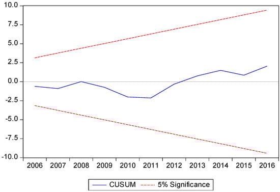
Figure 3.
Plot of CUSUM Test.
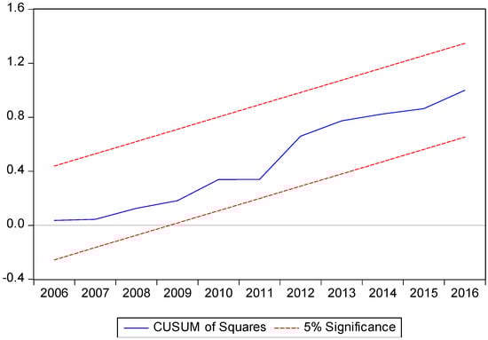
Figure 4.
Plot of CUSUMSQ Test.
3.4. VAR Estimation
Once an identified long-run structure is tested and fixed, the short run dynamics follows the long-run analysis. In order to further support the short run results of ARDL model we check the short run dynamic interactions among the variables by using a VAR model. As the main variables of our model are reported with unit roots, in VAR we take first difference for such variables account for the non-stationarity of the underlying data generating process. We estimate VAR analysis as follows:
where Xt is a vector of time series variables of real GDP, investment, private consumption, public consumption, trade openness, population growth and debt-to-GDP. Thus, Φ is a 7 × 7 matrix of coefficients, μ is a constant and et is a vector of random errors.
As a first step in the VAR estimation we shall make a choice regarding the optimal lag order j for the right-hand variables in the system of equations (Lütkepohl 2006). To determine the lag length of the VAR, three versions of the system were initially estimated: a four, a three and a two-lag version. Then, the Akaike information criterion identified one lag as optimal lag length. The VAR model passes all the standard diagnostic tests for residual autocorrelation, normality and heteroskedasticity.
Impulse Response Functions and Variance Decomposition Analysis
In order to study the dynamic properties of the model, impulse response function (IRF) analysis is applied. The IRF is the dynamic response of each dependent variable to other variables contained in the VAR model, for a standard deviation shock to the system. These functions show the effect of a one-time shock to one of the innovations on current and future values of the endogenous variables. In other words, this approach is designed to show how each variable responds over time to an earlier shock in that variable, and to shocks in other variables. The time period of IRF spreads over ten years, which is long enough to capture the dynamic interactions between GDP, investment, private consumption, public consumption, trade openness, debt-to-GDP and population growth. The IRFs are illustrated in Figure 5. First and foremost, it becomes apparent that the response of economic growth to a one standard deviation shock in investment, private consumption, public consumption and trade openness is positive, while is almost zero in population growth. On the other hand, a shock in debt-to-GDP has a negative impact on economic growth. The strongest positive impact arises from investment and private consumption to economic growth. Similarly, the response of investment, private consumption, public consumption, trade openness and population growth on a shock in economic growth is positive and substantial in magnitude. On the other hand, the response of debt-to-GDP to economic growth is negative. These results seem to be in agreement with those of the ARDL estimates.
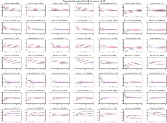
Figure 5.
Impulse Response Function (IRF). (Note: D indicates that the variables are expressed in first difference. GDP is the real GDP, GFCF is the gross fixed capital formation, GC is the final consumption expenditure of general government, IC is the private final consumption expenditure, trade is the trade openness-to-GDP ratio, debt is the debt-to-GDP ratio and POP is the population number in persons. The data selected from AMECO database for the time period 1970–2016.).
The variance decomposition (VDC) is next estimated for each variable for a period of ten years. VDC provides information about how much of the forecast error variance for each endogenous variable in the model can be explained by each disturbance. A shock to a particular variable will affect that variable directly, but this shock will also generate variations to all other variables in the system, through the dynamic structure of the model. The VDC estimation results for 10 years ahead are presented in Table 5.
Table 5.
Variance decomposition.
The variation of GDP is largely explained by its own innovations. As the years pass, firstly private consumption and secondly public consumption and investment, gradually affect more the variation of economic growth. More precisely, 3.20, 2.41 and 2.20 percent of economic growth forecast error variance in a ten years period is explained by disturbances of private consumption, public consumption and investment, respectively. Variations in investment are mainly explained by its own innovation and by innovation of GDP and debt. About 70 percent of investment forecast error variance in a ten years period is explained by disturbances of GDP. Private consumption’s variation is mainly explained by its own innovation and by innovation of GDP, public consumption and debt-to-GDP. Also, about 44 and 10 percent of public consumption forecast error variance in a ten years period is explained by disturbances of GDP and investment, respectively. Variations in trade openness are mainly explained by its own innovation and by innovation of GDP, private consumption and investment. Almost the half of debt-to-GDP’s variation is mainly explained by innovation of GDP, public and private consumption and investment and the other half due to its own innovation. Finally, variations in population growth are mainly explained by its own innovation and by innovation of GDP. These overall results seem to be in agreement with those of IRF.
3.5. Multiple Structural Breaks Model
Next, we apply a multi-step approach to our dataset covering the period 1970–2016 to analyze the link between government debt and growth. Following Bai and Perron (1998, 2003), a multiple linear regression with T periods and m potential breaks (producing m + 1 regimes) is considered by using the relationship of the following regression:
where, yt is the explained variable real GDP; debtt is the debt-to-GDP and Xt are the explanatory variables (investment, private consumption, public consumption, trade openness and population growth; βi and zi are the corresponding vectors of regime-dependent coefficients for i = 1,…,m + 1 and ut is the error term at time t.
3.5.1. Multiple Structural Breaks Tests
The number of significant breaks can be found via a sequential algorithm for multiple breaks model as Bai and Perron (1998, 2003) suggest. In a case of m breaks, while the first break point is identified, the sample is separated into two sub-samples by the first break point. The same procedure is employed for each sub-sample until the m breaks are arrived and the null hypothesis is not rejected for this m at the specified significance level (Table 6).
Table 6.
Tests for Breaks using the method of “m + 1” vs. “m” Breaks.
First the linear specification is tested against a one break model. The results from test showed that the null hypothesis of the linear model can be rejected against the alternative of one break model and the break date is 2007. Next, the null of one break model is tested against the alternative of two breaks model. Again the null of one break model against the alternative of two breaks model is rejected and the break dates are 1990, 2007. Next, the null of two breaks model is tested against the alternative of three breaks model. The null of the two breaks model against the alternative of three breaks model is rejected and the break dates are 1983, 1990, 2007. Next, the null of three breaks model is tested against the alternative of four breaks model. Again the null of the three breaks model against the alternative of a four breaks model is rejected and the break dates are 1983, 1990, 2000 and 2007. Finally, the four breaks model is tested against the alternative of a five breaks model and in this case the null hypothesis is not rejected.
3.5.2. Multiple Structural Breaks Estimation Results
Table 7 presents the results from the multiple structural break estimations over the period 1970–2016 for the Greek economy.
Table 7.
Estimation results of structural breaks analysis.
The break model for the period 1970–1982 shows that the growth of the Greek economy was mainly based on investment and private consumption. For the period 1983–1989 investment, private and government consumption have significant positive effects on economic growth, while the debt-to-GDP and trade has insignificant effects on economic growth. For the period 1990–1999 only private consumption and population growth have significant positive effects on economic growth, while the other variables have insignificant effects. For the period 2000–2006 a 10 percentage point rise in the debt-to-GDP goes in tandem with 8.4 percentage point decline in economic growth. Also, investment, private consumption, trade and population growth have significant positive effects on economic growth, while government consumption has insignificant negative effects. Finally, for the period 2007–2016 debt-to-GDP and population growth have insignificant effects on economic growth. On the other hand, investment, private and government consumption and trade have significant positive effects on economic growth. Our empirical findings are consistent with the results of the literature review (Reinhart and Rogoff 2010; Reinhart et al. 2012; Checherita-Westphal and Rother 2012; Furceri and Zdzienicka 2012).
4. Discussion of Research Findings
The empirical analysis reveals that the variables of GDP, investment, private and government consumption, trade openness, population growth and debt-to-GDP are co-integrated. This implies that long-run movements of the variables are determined by an equilibrium relationship. The role of the examined variables on economic growth seems to be significant. The results indicate that all variables have a positive contribution to economic growth, with the exception of debt-to-GDP and imports. Investment continues to significantly contribute to the increase of output growth. One of the most noticeable results is the high contribution of public and private consumption on economic growth. One explanation could be that the government and private expenditures have rapidly increased during the last four decades in Greece. Regarding the impact of debt-to-GDP on economic growth, we observe negative results for Greece. The negative effect of debt-to-GDP on growth means that domestic borrowing from foreign capital was used, partially, to finance government expenditure and public investment, thus contributing to the increase in public spending, increases budget deficit and leading to higher public debt in order to finance these deficits. Over recent decades the increase in consumption could not be financed out of current production. External borrowing in Greece was directed not for used in the industry, or for the other prospects for economic growth, but they were actually used for consumption. Therefore, the expansion in domestic demand (public and private) financed by the capital inflows was the main reason behind the loss of competitiveness in Greece.
Also, the results reveal that in Greece, the timing of the estimated break was at the year 2000. In this year the turning point of debt-to-GDP beyond which economic growth slows down sharply is 105% of GDP. Above the threshold of 105% of GDP levels of debt-to-GDP has had significant negative effect on growth and these results could explain why government debt was a significant drag on economic growth of Greece. The period 2000–2006 is associated with the period after the Euro currency was launched and before the beginning of the global financial crisis.
5. Conclusions
The impact of government debt on economic growth remains a controversial issue in both the academic and policy-making fields. This study empirically investigates the impact of debt-to-GDP and other economic determinants (investment, private and public consumption, trade openness and population growth) on economic growth of Greece, including the period of financial crisis. The results indicate that all variables in the long run have a positive contribution to economic growth, with the exception of debt-to-GDP and population growth. Also, by using structural breaks models, we found evidence in favor of a negative relationship between debt-to-GDP and growth. The main conclusion from the results is that the crisis in Greece had started much earlier than the global one.
The challenge for policy makers is to halt the rising in government debt by keeping a sustainable growth path. The recent global economic crisis showed that high government debt created huge fiscal imbalances in the Greek economy. Indeed, when government debt is high, this is perceived by investors as being extremely risky, creating difficulties on lending from the markets, leading to austerity fiscal policies, which deepens recession. For Greece, the financial market behavior over time has clearly shifted towards pessimism, insinuating that the risk attitude of major market participants has been altered. Regarding the impact of fiscal rules and institutions on market behavior, empirical findings show that they improve market’s expectations over fiscal sustainability (Apergis and Mamatzakis 2014; Mamatzakis and Tsionas 2015). As a result, enhancing fiscal governance could reduce the degree of the market’s pessimism regarding the Greek sovereign debt crisis. That is necessary because Greece needs to restore the liquidity of its banking system, by recovering the access to the international financial markets. The liquidity arrangement will help to boost liquidity in the domestic market and further to economic growth and the next step should be the end of the restrictions of capital controls. Therefore, Greece should reduce its deficits, increase its primary budget surplus and enhance the effectiveness of planning and operating policy to identify an optimal debt for support the growth of the country. To conclude, fiscal consolidation, adjustment and discipline, although necessary, are not, by themselves, a sufficient condition for economic growth and social welfare. To overcome the financial crisis, it is essential fiscal discipline to combine that with the implementation of coherent, consistent and sequential growth-enhancing structural reforms. For policymakers it is particularly important to select the appropriate macroeconomic tools to improve the situation of the Greek economy. Further improvements in competitiveness are important, which need to lower costs and shift resources to tradable sectors to spur growth and rebalance their external position (Spilimbergo et al. 2009). Thus, Greece should base its growth strategies on increasing exports, improving competitiveness and productivity, enhancing research and innovation, attracting foreign direct investment and correcting the use of public investment. Furthermore, simulations from a calibrated model of the Greek economy confirm that reforms to the labor markets can play a significant role in stemming output losses and supporting the recovery (International Monetary Fund 2013a, 2013b). Given that the debt accumulated during recent years is very large, the adjustment is likely to take a long time.
Further research is certainly needed to fully understand the impact of government debt on economic growth. One could probably investigate how the Greek debt crisis has affected the foreign exchange rate and interest rates. This could be a further analysis for the investigation of the relationship between GDP growth and debt-to-GDP. Many determinants of economic growth, as investments are dependent on interest rates and exports/imports are dependent on foreign exchange rate.
Conflicts of Interest
The author declares no conflict of interest.
References
- Afonso, Antonio, and José Ricardo Alves. 2015. The Role of Government Debt in Economic Growth. Hacienda Pública Española IEF 215: 9–26. [Google Scholar] [CrossRef]
- Afonso, António, and João Tovar Jalles. 2013. Growth and productivity: The role of government debt. International Review of Economics & Finance 25: 384–407. [Google Scholar]
- Akaike, Hirotugu. 1974. A new look at the statistical model identification. IEEE Transactions on Automatic Control 19: 716–23. [Google Scholar] [CrossRef]
- AMECO Database. 2017. Available online: http://ec.europa.eu/economyfinance/ameco/user/serie/SelectSerie.cfm (accessed on 30 November 2017).
- Anyanwu, John, and Andrew Erhijakpor. 2004. Domestic Debt and Economic Growth: The Nigerian Case. West African Financial and Economic Review 1: 98–128. [Google Scholar]
- Apergis, Nicholas, and Emmanuel Mamatzakis. 2014. What are the driving factors behind the rise of spreads and CDS of euro-area sovereign bonds? A FAVAR model for Greece and Ireland. International Journal of Economics and Business Research 7: 104–20. [Google Scholar] [CrossRef]
- Bai, Jushan, and Pierre Perron. 1998. Estimating and Testing Linear Models with Multiple Structural Changes. Econometrica 66: 47–78. [Google Scholar] [CrossRef]
- Bai, Jushan, and Pierre Perron. 2003. Computation and analysis of multiple structural change models. Journal of Applied Econometrics 18: 1–22. [Google Scholar] [CrossRef]
- Bökemeier, Bettina, and Alfred Greiner. 2015. On the relation between public debt and economic growth: An empirical investigation. Economics and Business Letters 4: 137–50. [Google Scholar]
- Brown, Robert L., James Durbin, and James M. Evans. 1975. Techniques for Testing the Constancy of Regression Relationships over Time. Journal of the Royal Statistical Society, Series B 37: 149–92. [Google Scholar]
- Checherita-Westphal, Cristina, and Philipp Rother. 2012. The impact of high government debt on economic growth and its channels: An empirical investigation for the euro area. European Economic Review 56: 1392–405. [Google Scholar] [CrossRef]
- Cuestas, Juan Carlos, Luis A. Gil-Alana, and Karsten Staehr. 2014. Government debt dynamics and the global financial crisis: Has anything changed in the EA12? Economics Letters 124: 64–66. [Google Scholar] [CrossRef]
- Dickey, David A., and Wayne A. Fuller. 1979. Distributions of the estimators for autoregressive time series with a unit root. Journal of American Statistical Association 74: 427–31. [Google Scholar]
- Dickey, David A., and Wayne A. Fuller. 1981. Likelihood ratio statistics for autoregressive time series with a unit root. Econometrica 49: 1057–72. [Google Scholar] [CrossRef]
- Drine, Imed, and M. Sami Nabi. 2010. Public external debt, informality and production efficiency in developing countries. Economic Modelling 27: 487–95. [Google Scholar] [CrossRef]
- Eberhardt, Markus, and Andrea F. Presbitero. 2015. Public debt and growth: Heterogeneity and non-linearity. Journal of International Economics 97: 45–58. [Google Scholar] [CrossRef]
- Egert, Balázs. 2015. Public debt, economic growth and nonlinear effects: Myth or reality? Journal of Macroeconomics 43: 226–38. [Google Scholar] [CrossRef]
- El-Mahdy, Adel M., and Neveen M. Torayeh. 2009. Debt Sustainability and Economic Growth in Egypt. International Journal of Applied Econometrics and Quantitative Studies 6: 21–55. [Google Scholar]
- Furceri, Davide, and Aleksandra Zdzienicka. 2012. How costly are debt crises? Journal of International Money and Finance 31: 726–42. [Google Scholar] [CrossRef]
- Gómez-Puig, Marta, and Simón Sosvilla-Rivero. 2015. The causal relationship between debt and growth in EMU countries. Journal of Policy Modeling 37: 974–89. [Google Scholar] [CrossRef]
- International Monetary Fund. 2013a. Euro Area Policies. Country Report No. 13/231. Washington: International Monetary Fund. [Google Scholar]
- International Monetary Fund. 2013b. Selected Issues Paper for Greece. Country Report No. 13/155. Washington: International Monetary Fund. [Google Scholar]
- International Monetary Fund. 2016. Fiscal Monitor. Available online: www.imf.org/external/pubs/ft/fm/2016/02/pdf/fm1602.pdf (accessed on 15 January 2018).
- Jiménez-Rodríguez, Rebeca, and Araceli Rodríguez-López. 2015. What Happens to the Relationship between Public Debt and Economic Growth in European Countries? Economics and Business Letters 4: 151–60. [Google Scholar] [CrossRef]
- Kumar, Manmohan, and Jaejoon Woo. 2010. Public Debt and Growth. International Monetary Fund Working Paper No. 10/174. Washington: International Monetary Fund. [Google Scholar]
- Lütkepohl, Helmut. 2006. Structural vector autoregressive analysis for cointegrated variables. Advances in Statistical Analysis, German Statistical Society 90: 75–88. [Google Scholar]
- MacKinnon, James G. 1996. Numerical distribution functions for unit root and cointegration tests. Journal of Applied Econometrics 11: 601–18. [Google Scholar] [CrossRef]
- Mamatzakis, Emmanuel, and Mike Tsionas. 2015. How are market preferences shaped? The case of sovereign debt of stressed euro-area countries. Journal of Banking & Finance 61: 106–16. [Google Scholar]
- Misztal, Piotr. 2010. Public Debt and Economic Growth in the European Union. Journal of Applied Economic Sciences 5: 292–302. [Google Scholar]
- Narayan, Paresh Kumar. 2005. The saving and investment nexus for China: Evidence fromcointegration tests. Applied Economics 37: 1979–90. [Google Scholar] [CrossRef]
- Newey, Whitney K., and Kenneth D. West. 1987. A Simple Positive Semi-Definite, Heteroskedasticity and Autocorrelation Consistent Covariance Matrix. Econometrica 55: 703–8. [Google Scholar] [CrossRef]
- Ogunmuyiwa, Michael Segun. 2011. Does External Debt Promote Economic Growth? Journal of Economic Theory 3: 29–35. [Google Scholar]
- Pattillo, Catherine A., Helene Poirson, and Luca A. Ricci. 2004. What Are the Channels through Which External Debt Affects Growth? International Monetary Fund Working Paper No. 04/15. Washington: International Monetary Fund. [Google Scholar]
- Perron, Pierre. 1989. The great crash, the oil price shock, and the unit root hypothesis. Econometrica 57: 1361–401. [Google Scholar] [CrossRef]
- Perron, Pierre. 1997. Further evidence on breaking trend functions in macroeconomic variables. Journal of Econometrics 80: 355–85. [Google Scholar] [CrossRef]
- Pesaran, M. Hashem, Yongcheol Shin, and Richard J. Smith. 2001. Bounds Testing Approaches to the Analysis of Level Relationships. Journal of Applied Econometrics 16: 289–326. [Google Scholar] [CrossRef]
- Pescatori, Andrea, Damiano Sandri, and John Simon. 2014. Debt and Growth: Is There a Magic Threshold? International Monetary Fund Working Paper No. 14/34. Washington: International Monetary Fund. [Google Scholar]
- Reinhart, Carmen, and Kenneth Rogoff. 2010. Growth in a Time of Debt, American Economic Review. American Economic Association 100: 573–78. [Google Scholar]
- Reinhart, Carmen M., Vincent R. Reinhart, and Kenneth S. Rogoff. 2012. Public Debt Overhangs: Advanced-Economy Episodes since 1800. Journal of Economic Perspectives 26: 69–86. [Google Scholar] [CrossRef]
- Schclarek, Alfredo. 2004. Debt and Economic Growth in Developing and Industrial Countries. Working Papers 2005: 34. Lund: Lund University, Department of Economics. [Google Scholar]
- Schneider, Friedrich. 2011. The Shadow Economy Labour Force. World Economics 12: 53–92. [Google Scholar]
- Sen, Swapan, Krishna M. Kasibhatla, and David B. Stewart. 2007. Debt Overhang and Economic Growth the Asian and the Latin American Experiences. Economic Systems 31: 3–11. [Google Scholar] [CrossRef]
- Shah, Mahmud Hasan, and Pervin Shahida. 2012. External Public Debt and Economic Growth: Empirical Evidence from Bangladesh. Academic Research International 3: 508–15. [Google Scholar]
- Spilimbergo Antonio, Alessandro Prati, and Jonathan David Ostry. 2009. Structural Reforms and Economic Performance in Advanced and Developing Countries. International Monetary Fund Occasional Paper No. 268. Washington: International Monetary Fund. [Google Scholar]
- Swamy, Vighneswara. 2015a. Government Debt and Economic Growth—Decomposing the Cause and Effect Relationship. MPRA Paper 64105. Amsterdam: Elsevier. [Google Scholar]
- Swamy, Vighneswara. 2015b. Government Debt and its Macroeconomic Determinants—An Empirical Investigation. MPRA Paper 64106. Amsterdam: Elsevier. [Google Scholar]
- Tchereni, Betchani, Tshediso Joseph Sekhampu, and Roosevelt Ndovi. 2013. The Impact of Foreign Debt on Economic Growth in Malawi. African Development Review 25: 85–90. [Google Scholar] [CrossRef]
© 2018 by the author. Licensee MDPI, Basel, Switzerland. This article is an open access article distributed under the terms and conditions of the Creative Commons Attribution (CC BY) license (http://creativecommons.org/licenses/by/4.0/).