Aerial Footage Analysis Using Computer Vision for Efficient Detection of Points of Interest Near Railway Tracks

Abstract

Object detection is a fundamental part of computer vision, with a wide range of real-world applications. It involves the detection of various objects in digital images or video. In this paper, we propose a proof of concept usage of computer vision algorithms to improve the maintenance of railway tracks operated by Via Rail Canada. Via Rail operates about 500 trains running on 12,500 km of tracks. These tracks pass through long stretches of sparsely populated lands. Maintaining these tracks is challenging due to the sheer amount of resources required to identify the points of interest (POI), such as growing vegetation, missing or broken ties, and water pooling around the tracks. We aim to use the YOLO algorithm to identify these points of interest with the help of aerial footage. The solution shows promising results in detecting the POI based on unmanned aerial vehicle (UAV) images. Overall, we achieved a precision of 74% across all POI and a mean average precision @ 0.5 (mAP @ 0.5) of 70.7%. The most successful detection was the one related to missing ties, vegetation, and water pooling, with an average accuracy of 85% across all three POI.

1. Introduction

Railways are a crucial part of the modern world, as they help provide affordable public transport and facilitate the supply chain of goods essential for the current lifestyle. Railway tracks span thousands of kilometres, and maintaining these tracks is not easy for several reasons [1]. The first and most obvious reason is that these tracks pass through some of the most remote areas, which is beneficial in terms of connectivity, but, which also makes their surveillance and monitoring quite tricky, as some of the areas through which they pass are not easily accessible and require additional resources. Second, it also requires railway companies to employ a large workforce to ensure smooth operations and the general public’s safety [1].

One of the most crucial parts of railway track maintenance is the identification of sections that need to be repaired. Via Rail operates more than 500 trains per week in several Canadian provinces and 12,500 kilometres (7800 mi) of track [2]. The current approach requires regular manual monitoring of the tracks, which is resource-intensive. One of the crucial points of interest (POI) involves identifying vegetation that grows on the sided of the tracks, which could be fatal if not treated in a timely manner [3]. Identifying missing and broken wooden ties is an important task to increase the lifetime and operability of the tracks. Rainy weather could contribute to the sudden accumulation of water near tracks that is extremely difficult to identify quickly [4]. Advancements in certain technologies could revolutionize the identification of these points of interest.

Unmanned aerial vehicle (UAV) or remotely piloted aircraft system (RPAS) technology has essentially opened new opportunities for railway operators, offering safety and dependability, as well as reliable support [5]. The increased safety of workers is now commendable with UAVs on the rail sector side. With its arrival, the activities of the railways that previously required personnel to participate in dangerous inspection scenarios are no longer a problem. Integration of premium UAVs, advanced sensors, high-resolution cameras, and artificial intelligence (AI) has allowed this transportation industry to capture real-time data and perform intelligent data analysis.

The following are the main contributions of this paper.

• Approach: We study and apply the YOLOv5 object detection algorithm to detect various POI, that is, broken ties, missing ties, vegetation, and water pooling around railway tracks.
• Experimentation: We collected aerial image footage in 4K resolution and the top-down angle for training and testing purposes by using DJI Inspire 2 with a Zenmuse X7 camera in the Ottawa, ON, Canada region. Our research team performed annotations with the help of an expert from Transport Canada.
• Evaluation: We evaluate the algorithm’s accuracy by measuring how accurately it determines a particular POI. We consider precision, recall, and mean average precision to determine overall efficiency. In general, we achieved a precision of 74% and a mean average precision @ 0.5 (mAP @ 0.5) of 70.7%.

To the best of our knowledge, this is the first paper that applies the newest YOLOv5 model to detect various POI along the train tracks. It is also the first paper that proposes the detection of water pooling as one of the POI around train tracks from the aerial perspective.

The remainder of the paper is divided in the following way. In the next section, we discuss related works and compare them with our approach. We then provide an overview of the chosen approach in Section 3 and Section 4. Finally, we present the results and the detection examples in Section 5, followed by conclusions and plans for future work.

2. Related Work

The evolution of computer vision capabilities has made it possible to identify particular objects from various media sources, such as images and live streaming of videos [6,7,8,9,10,11]. One of the first papers on railway track object detection was proposed by Yuan et al. They used the enhanced Ostu algorithm to segment the rail picture and calculated the rail surface area, although the selection of thresholds for this method was not uniform [12]. Others offered a way to directly extract points of interest on the rail surface by improving the value by reducing the maximum variance between classes, although the precision of the recommended approach was not perfect [13]. In this section, we are going to discuss the related works and compare them with our approach.

The authors of [14] aim to provide a low-cost, practical framework for autonomous railway track detection by utilizing video cameras and computer vision algorithms. A computer vision technique is employed for the automatic detection of railroad lines. As part of the camera calibration operation, interior orientation characteristics are extracted. The external orientation parameters are computed by using the bundle adjustment calibration approach based on chosen ground control points. As a result, the eye fish effect of the photos is eliminated, and matching and feature extraction methods are used to create orthogonal images for the railway lines. The study provides a unique perspective on image pre-processing, which motivated similar implementation in this paper for correcting the orientation of images before the annotation process.

An algorithm for the detection of railway infrastructure objects, namely, track and signals, is proposed by [15] to detect signals relevant to the track and check if the train is moving along. The convolutional neural network based on the You Only Look Once technique, Hough transform, and other well-known computer vision algorithms are included in the algorithm. The principles of CV and CNNs each deal with a distinct object of detection, and when combined, they create a singular system that tries to identify both the rails and the relevant signals. By using this strategy, the artificial intelligence (AI) system is “aware” of the signal’s course. According to the experiments that were run, the proposed algorithm has an up to 99.7% accuracy rate for signal detection. Although this paper uses an algorithm similar to that used in [15], the target POI are different, and the application requires a more lightweight model to perform high-speed detection, which would not be possible with the same model as in [15].

Rails, fasteners, and other elements of railway track lines invariably develop flaws due to continuous pressure from train operations and direct exposure to the environment, which directly affects the safety of train operations. The study from [16] developed a multiobject detection approach to detect fastener and rail surface faults without causing damage. It is based on deep convolutional neural networks. The enhanced YOLOv5 framework first localizes the rails and fasteners on the train track image. The rail’s surface defects are then detected by using the defect detection model based on Mask R-CNN, and the defect area is segmented. The fasteners’ status is finally classified by using a model built on the ResNet framework. The application of the YOLOv5 model for fastener and fault detection inspired and confirmed the validity of the application of YOLOv5 to detect the POI in our study. Again, the POI that we refer to are different.

A review study conducted by Lei Kou [17] further explores the recent research done to address defect detection on the railway lines. Computer vision and deep learning methods, along with traditional ultrasonic and acceleration detection methods, are proposed to evaluate the damage to the rail surface that can drastically improve the efficiency of the detection system while reducing inspection costs. A similar approach is explored by M. Hashmi et al. in [18] where they combined traditional acoustic-based systems with deep learning models to improve performance and prevent railway accidents. In this regard, two CNN models, convolutional 1D and convolutional 2D, and one recurrent neural network (RNN) model are utilized. Initially, three fault types are considered: superelevation, wheel burned, and standard tracks. On-the-fly feature extraction is performed by creating spectrograms as a deep learning model’s layer. Because visual inspection is employed to identify POI in the current study, no traditional techniques were utilized.

In the past, methods based on computer vision have been investigated to detect flaws in railroad tracks. Still, full automation has always been challenging because neither conventional image-processing techniques nor deep learning classifiers trained from scratch perform well when applied to an infinite number of novel scenarios encountered in the real world when given a small amount of labeled data. Recent developments have made it possible for machine learning models to use data from an unrelated but relevant domain. The authors of [19] demonstrate that despite the lack of comparable domain data, transfer learning still allows for training large-scale deep learning classifiers on uncontrolled, real-world data and helps models understand other real-world objects. Similar transfer learning was employed in this study by using weights from previous training to improve accuracy and deal with a smaller dataset.

Another application of computer vision in the railway domain is detecting static objects. The study by Ye et al. [20] suggests a line-side condition monitoring strategy for the switch rail. The state of the switch rail, including movement, position, toe gap, and toe edge, can be remotely monitored in real-time by using specialized identification algorithms. Similarly, an intrusion-detecting algorithm for a railway crossing was suggested in [21]. The following three steps make up their procedure. First, three nonparametric background models for detecting moving and stationary objects were created, each with a different learning rate. An object-tracking approach is introduced to decrease false positives in the detection. The removal of static objects is followed by introducing a feedback mechanism to update the background models selectively. Although this approach was proven to be effective, our POI differ, and no correlation is found.

Tiange Wang, Fangfang Yang, and Kwok-Leung Tsui in [22] used the YOLO one-stage detection model to detect rail, clip, and bolt-on railway tracks. Bolts connect the ends of the rails at the joints, and elastic clips are used with the rail sleeper to connect the rails. Their approach used the k-means clustering method to discover the best aspect ratios of the previous boxes with the distance metric changed to 1-IoU. In [23] the authors used computer vision algorithms to detect cracks in the rail track plate. This was the only POI similar to the work done in this paper. Moreover, many other authors focused on a similar problem of crack detection [24]. To the best of our knowledge, this is the first paper that proposes the detection of water pooling as one of the POI around the train tracks.

Although the research in the area of railway track maintenance has been done recently, we want to reiterate that to the best of our knowledge, this is the first paper that applies the newest YOLOv5 model to detect broken and missing ties, as well as vegetation. It is also the first paper that proposes the detection of water pooling as one of the POI around the train tracks from the aerial perspective.

3. Algorithm Overview

YOLO (You Only Look Once) reframes object detection as a single regression problem rather than a classification problem. A single convolutional network simultaneously predicts multiple bounding boxes and class probabilities for the boxes shown in Figure 1.

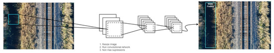
Figure 1. YOLO object detection.

YOLO makes global decisions about an image when making predictions. It sees the entire image during training and testing, so it implicitly encodes contextual information about classes, and their appearance [25]. We decided to choose the YOLO algorithm versus the single-shot multi-box detection (SSD) [26] for of two reasons. The first one was the speed of the detection. Our preliminary experiments showed that the YOLO algorithm offered a much higher detection speed with precision that was not much lower. The SSD’s algorithm speed was lower as our model was large and complex. Moreover, the SSD algorithm was slightly less accurate in detecting smaller objects, such as tie cracks. We will discuss more details of YOLO architecture in the following subsections.

3.1. Detection

The entire process is shown in Figure 2. The input image is divided into an S ∗ S grid. If the center of an object falls into a grid cell, that grid cell is responsible for detecting the object. Each cell in the grid predicts the B bounding boxes and the confidence scores for those boxes. Confidence is defined as P${}_r$(Object) ∗ IOU(truth, pred). The confidence score is zero if there is no object in that cell. Otherwise, the confidence score equals the intersection over union (IOU) between the predicted box and the ground truth.

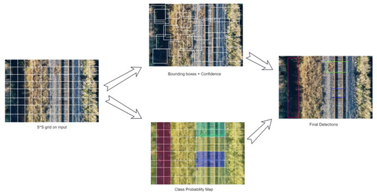
Figure 2. Bounding boxes creation with YOLO.

Each bounding box consists of five predictions: x, y, w, h, and confidence. The (x, y) coordinates represent the box’s center relative to the grid cell’s bounds. The (w, h) coordinates represent the width and height of the bounding box and are predicted relative to the entire image. Finally, confidence prediction represents the intersection over union (IOU) between the predicted and ground-truth boxes.

Each grid cell also predicts C conditional class probabilities—P${}_r$(Class${}_i$| Object). These probabilities are conditioned on the grid’s cell that contains an object. Only one set of class probabilities is predicted per grid cell, regardless of the number of boxes. In the test, the conditional class probabilities and the confidences of the individual box are multiplied by the following equation:

$$\begin{array}{c}\hfill P_r\left(Clas{s}_i|Object\right)\ast P_r\left(Object\right)\ast IO{U}_{pred}^{truth}=\\ \hfill P_r\left(Clas{s}_i\right)\ast IO{U}_{pred}^{truth}\end{array}$$

(1)

3.2. Architecture

The YOLO model is implemented as a convolutional neural network. The initial convolutional layers of the network extract features from the image, whereas the fully connected layers predict the output probabilities and coordinates. The detection network architecture has 24 convolution layers and two fully connected convolution layers. Alternating $1\times 1$ convolution layers reduce the preceding layers’ feature space. The network is shown in Figure 3.

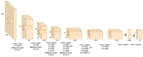
Figure 3. Architecure of YOLO.

3.3. Activation and Loss Function

The final layer predicts both class probabilities and bounding box coordinates. The coordinates of the bounding box are then normalized to 0 and 1. A linear activation function for the final layer and all other layers uses the following leaky rectified linear activation:

$$\varphi \left(x\right)=\left\{\begin{array}{ccc}x,& ifx>0& \\ 0.1x,& otherwise\end{array}\right\}.$$

(2)

The sum-square error in the output of the loss function is optimized by using Equation (3).

$$\begin{array}{c}\hfill {\lambda }_{coord}\sum _{i=0}^{S^2}\sum _{j=0}^B{1}_{ij}^{obj}\left[{\left(x_i-{\widehat{x}}_i\right)}^2+{\left(y_i-{\widehat{y}}_i\right)}^2\right]+\\ \hfill {\lambda }_{coord}\sum _{i=0}^{S^2}\sum _{j=0}^B{1}_{ij}^{obj}\left[{\left(\sqrt{w_i}-\sqrt{{\widehat{w}}_i}\right)}^2+{\left(\sqrt{h_i}-\sqrt{{\widehat{h}}_i}\right)}^2\right]\\ \hfill +\sum _{i=0}^{S^2}\sum _{j=0}^B{1}_{ij}^{obj}{\left(C_i-{\widehat{C}}_i\right)}^2+\\ \hfill {\lambda }_{noobj}\sum _{i=0}^{S^2}\sum _{j=0}^B{1}_{ij}^{noobj}{\left(C_i-{\widehat{C}}_i\right)}^2+\\ \hfill \sum _{i=0}^{S^2}{1}_i^{obj}\sum _{c\epsilon classes}{\left(p_i\left(c\right)-{\widehat{p}}_i\left(c\right)\right)}^2\end{array}.$$

(3)

Here, $S^2$ is an $S\times S$ grid created by YOLO for detection, B is a bounding box, $1_i^{obj}$ denotes if an object is present in cell i, $1_{ij}^{obj}$ denotes $j_{th}$ the bounding box responsible for the prediction of the object in the cell i, and finally ${\lambda }_{coord}$, $lambd{a}_{noobj}$ are regularization parameters required to balance the loss function. $x_i$,$y_i$ denotes the location of the center of the bounding box, $w_i$,$h_i$ denotes the width and height of the bounding box, $C_i$ denotes the confidence score of whether there is an object or not and $p_i\left(c\right)$ denotes classification loss.

3.4. YOLOv5

The architecture of YOLOv5 consists of three parts (as shown in Figure 4). These are the backbone (CSPDarknet), the neck (PANet), and the head (YOLO layer). The data is first inputted to CSPDarknet for feature extraction and then fed to PANet for feature fusion. Finally, the YOLO layer outputs detection results (class, score, location, size) [27].

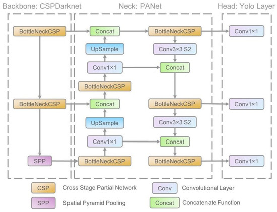
Figure 4. Architecture of YOLOv5.

Joseph Redmon (inventor of YOLO) introduced the anchor box structure in YOLOv2 and a procedure for selecting anchor boxes of size and shape that closely resemble the ground-truth bounding boxes in the training set. By using the k-means clustering algorithm with different k values, the authors picked the five best-fit anchor boxes for the COCO dataset (containing 80 classes) and used them as a default. This reduces training time and increases network accuracy.

However, when applying these five anchor boxes to a unique dataset (containing a class not present in the original COCO datasets), these anchor boxes cannot quickly adapt to the ground-truth bounding boxes of this unique dataset. For example, a giraffe dataset prefers anchor boxes with thin and higher shapes than a square box. To address this problem, computer vision engineers usually run the k-means clustering algorithm on the unique dataset to get the best-fit anchor boxes for the data first. These parameters will then be manually configured in the YOLO architecture.

Glenn Jocher (inventor of YOLOv5) proposed integrating the anchor box selection process into YOLOv5. As a result, the network does not have to consider any of the datasets to be used as input; it will automatically “learn” the best anchor boxes for that dataset and use them during training [27].

4. Methodology

Figure 5 shows the model pipeline with each step involved, from data collection to image inference processing, in our research study. Data was collected by using a UAV during flights over the Ottawa region in the fall of 2021. High-resolution images were captured from various distances [25 m, 50 m, 75 m]. After performing data pre-processing, the RoboFlow tool was used to annotate the POI. Roboflow also enabled the augmentation (vegetation only) and versioning of the dataset. After creating the dataset package in Roboflow, the Google Colab notebook was used to run algorithms for the model’s training in connection to Amazon Web Server external instance. Once the model was trained, the trained weights were extracted and used for inference on the images.

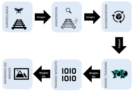
Figure 5. Model pipeline.

4.1. Dataset Pre-Processing

Dataset pre-processing is performed to ensure that the data are in the suitable format for the algorithm’s training. After an initial assessment, the following pre-processing steps were performed on the dataset to enable efficient annotation, which is critical for machine learning model performance:

• Image Orientation Correction. To make the annotation process more manageable and efficient, the orientation of the images was corrected so that the tracks were in a vertical or horizontal direction. Moreover, all images were taken by using the top-down approach to prevent the situation where different angles of the image affect the detection quality.
• Artificial Vegetation. As the rail tracks are well maintained, there were very few images in which vegetation was visible. To achieve higher accuracy, we needed to train the model by using a well-balanced set of images with points of interest; thus, artificial vegetation was added on and beside the tracks.

4.2. Annotation

After pre-processing the data, the next step was to annotate the images to train the algorithm. We identified four points of interest:

• Vegetation: Each image was closely reviewed to check for vegetation near the track. If it was present at a distance from the track (<3 m), it was annotated accordingly. An example is shown in Figure 6.
  

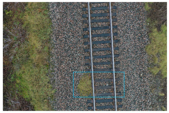  Figure 6. Example of vegetation.
• Missing Tie: The track portion was annotated when there was a missing tie. An example is shown in Figure 7.
  

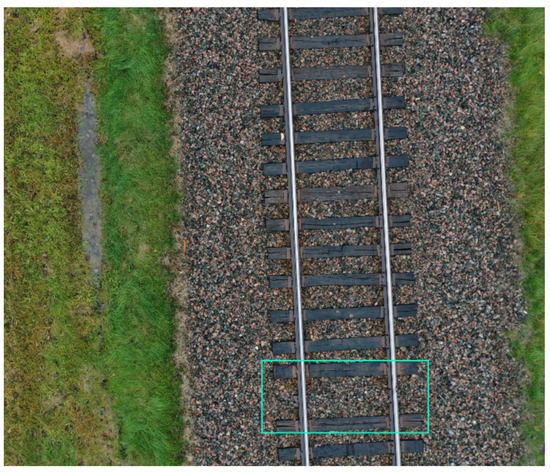  Figure 7. Example of a missing tie.
• Broken Tie: If there was a crack at least 50% of the length of the tie (calculated horizontally), the tie was annotated as a broken one. An example is shown in Figure 8.
  

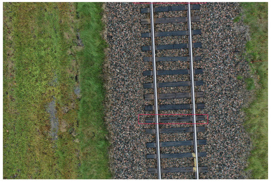  Figure 8. Example of a broken tie.
• Water Pooling: Any water body captured in the images was annotated as water pooling to identify the sites affected by water pooling near the tracks. An example is shown in Figure 9.
  

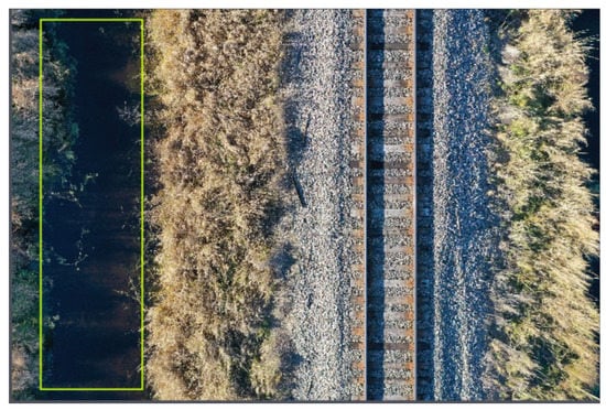  Figure 9. Example of water pooling.

4.3. Simulation Setup

In this section, we discuss the simulation parameters and share additional details on the collected dataset. The total number of images used in the simulations was 5465, as shown in Figure 10. On average, we had two annotations per image, and a median image ratio of 5472 × 3648 collected from multiple UAVs.

Figure 10. Dataset Health Check.

Moreover, we present a class balance in Figure 11. We performed an analysis in Roboflow, and none of the classes were under- or over-represented. The largest collection of images was marked with a water pooling class annotation.

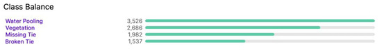
Figure 11. Class balance.

Finally, for each class, we present the distribution of annotations per image, for water pooling, vegetation, missing ties, and broken ties, in Figure 12, Figure 13, Figure 14 and Figure 15, respectively. As we can see, the water pooling objects appeared as multiple instances on the images, whereas the rest of the classes were mostly individual objects per singular image.

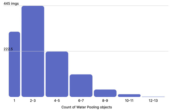
Figure 12. Distribution of water pooling objects per image.

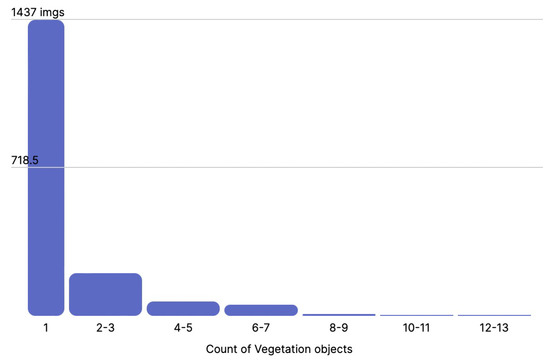
Figure 13. Distribution of vegetation objects per image.

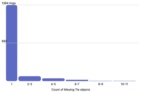
Figure 14. Distribution of missing tie objects per image.

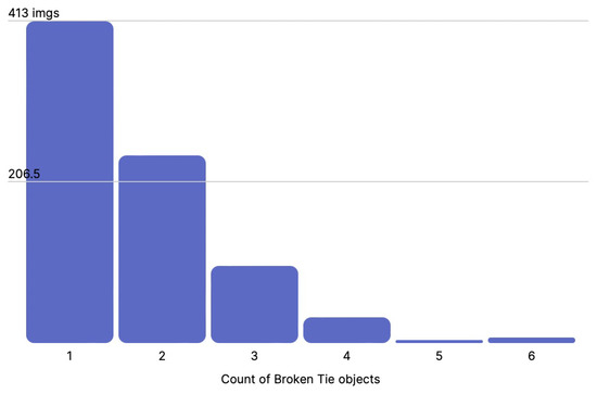
Figure 15. Distribution of broken tie objects per image.

We used 70% images for training purposes, 20% images for validation, and 10% images for testing purposes. We trained the YOLOv5m6 model from scratch with images resized to 640 pixels, in batches of 32, for 300 epochs, in an offline matter (images were taken by UAVs, then transferred to the server and used for training and testing). Our “patience” argument for training was set to 100 epochs, resulting in the training procedure stopping around 180 epochs due to no further model improvement. We used the hyperparameter settings shown in Table 1. The number of warm-up epochs was set to 5. The detection threshold was set to 0.7. In the next section, we discuss the results of the simulations.

Table 1. Hyperparameters.

Hyperparameter	Target Value	Warmup Value
Learning Rate	0.1	0.1
Detection Threshold	0.7	0.7
Momentum	0.937	0.8
Weight Decay	0.0005	N/A

5. Results

During model training, many different experiments were performed to optimize the performance of each point of interest by analyzing the initial results. In general, we achieved a precision of 74.1% and 70.7% mAP for detecting all classes, as shown in Table 2.

Table 2. Results of the simulations.

Class	Labels	Precision	Recall	mAP@.5
All	1936	0.741	0.61	0.707
Broken Tie	327	0.503	0.595	0.455
Missing Tie	377	0.89	0.814	0.882
Vegetation	558	0.84	0.667	0.807
Water Pooling	674	0.809	0.765	0.742

One of our model’s tasks was detecting broken ties on railway tracks. For the class of a broken tie, we achieved the lowest precision among all other classes, equal to 50.3% precision and 59.5% mAP.

During the initial phases of model training, the image dataset consisted of images taken from greater height [50–70 m], which contributed to lower performance, as identifying cracks in the ties was difficult due to lower resolution. Therefore, it was recommended that UAV images be taken from a lower height [25 m] to achieve optimal results. Pictures taken from higher heights were removed from the dataset. As a result of these changes, a 7% improvement in performance was witnessed but remained on a lower level than expected. Overall, the detection performance of broken ties remained average due to various factors affecting the algorithms’ ability to detect broken ties. These factors involved mainly a high variation in cracks (due to the type of material—wood) and a low number of repeated samples for each type of crack. All of these factors affect the appearance of cracks in the tie. We are confident that with a larger dataset of more standardized cracks, we could introduce a different level of damage severity identified in training classes to improve overall results in this category.

Another task was to detect missing ties. We achieved the highest precision among all classes in this category—89% and the highest mAP—88.2%. This class was the easiest to detect because of an evident visual change in the tracks. By enabling tracking the distance between two ties, we could quickly identify missing ones, which can also help prioritize the maintenance of railway tracks.

Furthermore, one POI was to detect vegetation. For this class, we achieved 84% detection precision and 80.7% mAP. Further research in the vegetation category could involve mapping the size of vegetation or tracking the level/amount of ballast to implement effective deterrence against vegetation growth.

Finally, we focus on the most significant issue, water pooling. Our model achieved 80.9% detection precision and 74.2% mAP. Achieving high precision in the case of water pooling is extremely difficult, but we overcame the issue by using appropriate pre-processing methods, such as adaptive equalization of contrast and correction of white balance (including tint adjustment). In some cases, we observed that the exact area of water pooling did not match the boundary boxes perfectly, but the overall detection goal was very accurate.

Example Results of Detection

One of our model’s tasks was detecting vegetation near railway tracks. Our model detects vegetation near tracks with high accuracy, as shown in Figure 16. The model does not detect vegetation when it is sparse in the entire area near the railway track, as shown in Figure 17.

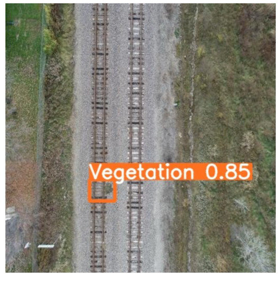
Figure 16. Positive vegetation detection.

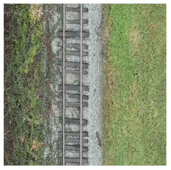
Figure 17. Negative vegetation detection.

Missing ties are detected accurately by our model, as shown in Figure 18. Our model does not detect missing ties when the distance between the missing ties is uneven (see Figure 19).

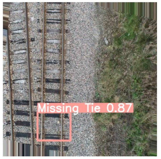
Figure 18. Positive missing tie detection.

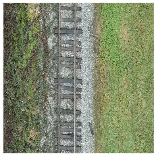
Figure 19. Negative missing tie detection.

The model detects broken ties correctly as shown in Figure 20. It does not detect broken ties when the broken part contains gravel, as shown in Figure 21.

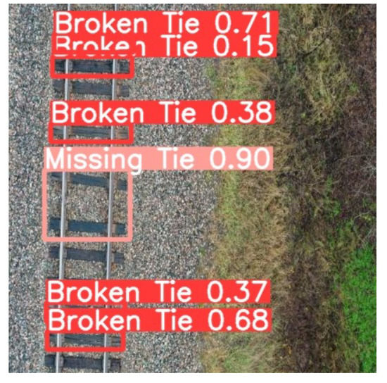
Figure 20. Positive broken tie detection.

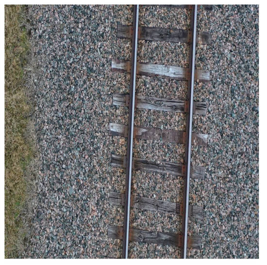
Figure 21. Negative broken tie detection.

Water pooling is detected with high accuracy, as shown in Figure 22. Figure 23 shows an example of not perfectly accurate detection, where the water has a dark reflection.

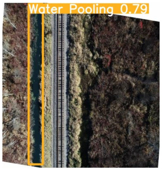
Figure 22. Positive water pooling detection.

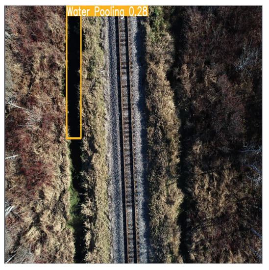
Figure 23. Negative water pooling detection.

6. Conclusions

In this article, we tackled the problem of identifying various points of interest around railway tracks by using aerial image footage. We processed them by using the YOLO object detection algorithm. The algorithm’s efficiency was evaluated by measuring how accurately it determines the specific points of interest.

The accuracy of detecting various points of interest was directly proportional to the height at which the aerial footage was taken. For example, images with broken ties were challenging to identify from a greater distance. In addition, the algorithm quickly identified vegetation and missing ties in the images from various distances due to the more significant visual features of those classes. Finally, the water pooling was detected efficiently. As a next step, we are going to include images from different seasons of the year and more locations to improve the accuracy of the solution. As an end product, the algorithms developed in this paper have been deployed in production-ready software called Spexi Geospatial.

6.1. Major Achievements

• The model achieved more than 80% accuracy in categories such as vegetation, missing ties, and water pooling.
• YOLOv5 offers a faster inference time than YOLOv4, allowing for deployment on embedded devices.
• The deployment of the model by the railway maintenance department could significantly reduce the time and resources required for detecting major POI.

6.2. Limitations

• The model does not perform well for the broken tie class due to the lack of distinct, standardized visual features and false identification resulting from ballasts on ties.
• The model lacks terrain diversity in the training dataset, which could result in lower accuracy for different geographic locations.

7. Future Work

In future work, we plan to conduct more robust training that includes images from diverse landscapes and seasons of the year to improve accuracy and make the model production-ready. Moreover, more research is required to handle the identification of visual features for specific categories, such as a broken tie. Visual feature enhancement can be performed during the pre-processing step to improve accuracy. Finally, the augmentation technique could be customized to reduce noise from the image by colour coding the unwanted areas.

References

- Chenariyan Nakhaee, M.; Hiemstra, D.; Stoelinga, M.; van Noort, M. The Recent Applications of Machine Learning in Rail Track Maintenance: A Survey. In Reliability, Safety, and Security of Railway Systems. Modelling, Analysis, Verification, and Certification; Collart-Dutilleul, S., Lecomte, T., Romanovsky, A., Eds.; Springer International Publishing: Cham, Switzerland, 2019; pp. 91–105. [Google Scholar]
- Rail, V. Annual Report 2021. Available online: https://media.viarail.ca/sites/default/files/publications/Annual_Report_2021.pdf (accessed on 1 May 2022).
- Rahman, M.; Mammeri, A. Vegetation Detection in UAV Imagery for Railway Monitoring. In Proceedings of the VEHITS Conference, Online, 28–30 April 2021. [Google Scholar]
- Kellermann, P.; Schönberger, C.; Thieken, A.H. Large-scale application of the flood damage model RAilway Infrastructure Loss (RAIL). Nat. Hazards Earth Syst. Sci. 2016, 16, 2357–2371. [Google Scholar] [CrossRef] [Green Version]
- Aibin, M.; Aldiab, M.; Bhavsar, R.; Lodhra, J.; Reyes, M.; Rezaeian, F.; Saczuk, E.; Taer, M.; Taer, M. Survey of RPAS Autonomous Control Systems Using Artificial Intelligence. IEEE Access 2021, 9, 167580–167591. [Google Scholar] [CrossRef]
- Bengio, Y. Learning Deep Architectures for AI. Found. Trends® Mach. Learn. 2009, 2, 1–127. [Google Scholar] [CrossRef]
- Hu, Y.; Xu, X.; Ou, Z.; Song, M. A Crowdsourcing Repeated Annotations System for Visual Object Detection. In Proceedings of the 3rd International Conference on Vision, Image and Signal Processing, Vancouver, BC, Canada, 26–28 August 2019. [Google Scholar] [CrossRef]
- Wu, J.; Shi, H.; Wang, Q. Contrabands Detection in X-ray Screening Images Using YOLO Model. In ACM International Conference Proceeding Series; ACM Press: New York, NY, USA, 2020. [Google Scholar] [CrossRef]
- Xu, R.; Lin, H.; Lu, K.; Cao, L.; Liu, Y. A Forest Fire Detection System Based on Ensemble Learning. Forests 2021, 12, 217. [Google Scholar] [CrossRef]
- Karimibiuki, M.; Aibin, M.; Lai, Y.; Khan, R.; Norfield, R.; Hunter, A. Drones’ Face off: Authentication by Machine Learning in Autonomous IoT Systems. In Proceedings of the IEEE 10th Annual Ubiquitous Computing, Electronics and Mobile Communication Conference, (UEMCON 2019), New York, NY, USA, 1–4 December 2019; pp. 329–333. [Google Scholar] [CrossRef]
- Vinchoff, C.; Chung, N.; Gordon, T.; Lyford, L.; Aibin, M. Traffic Prediction in Optical Networks Using Graph Convolutional Generative Adversarial Networks. In Proceedings of the International Conference on Transparent Optical Networks, Bari, Italy, 19–23 July 2020; pp. 3–6. [Google Scholar]
- Yuan, X.C.; Wu, L.S.; Peng, Q. An improved Otsu method using the weighted object variance for defect detection. Appl. Surf. Sci. 2015, 349, 472–484. [Google Scholar] [CrossRef] [Green Version]
- Min, Y.; Xiao, B.; Dang, J.; Yue, B.; Cheng, T. Real time detection system for rail surface defects based on machine vision. Eurasip J. Image Video Process. 2018, 2018, 1–11. [Google Scholar] [CrossRef] [Green Version]
- Adham, M.; Mohamed, G.; El-Shazly, A. Railway Tracks Detection of Railways Based on Computer Vision Technique and GNSS Data; MDPI: Basel, Switzerland, 2020. [Google Scholar] [CrossRef]
- Petrović, A.D.; Banić, M.; Simonović, M.; Stamenković, D.; Miltenović, A.; Adamović, G.; Rangelov, D. Integration of Computer Vision and Convolutional Neural Networks in the System for Detection of Rail Track and Signals on the Railway. Appl. Sci. 2022, 12, 45. [Google Scholar] [CrossRef]
- Zheng, D.; Li, L.; Zheng, S.; Chai, X.; Zhao, S.; Tong, Q.; Wang, J.; Guo, L. A Defect Detection Method for Rail Surface and Fasteners Based on Deep Convolutional Neural Network. Comput. Intell. Neurosci. 2021, 2021, 5500. [Google Scholar] [CrossRef] [PubMed]
- Kou, L. A Review of Research on Detection and Evaluation of Rail Surface Defects. EasyChair 2021, 7244, 20. [Google Scholar] [CrossRef]
- Hashmi, M.S.A.; Ibrahim, M.; Bajwa, I.S.; Siddiqui, H.U.R.; Rustam, F.; Lee, E.; Ashraf, I. Railway Track Inspection Using Deep Learning Based on Audio to Spectrogram Conversion: An on-the-Fly Approach. Sensors 2022, 22, 1983. [Google Scholar] [CrossRef] [PubMed]
- Mittal, S.; Rao, D. Vision Based Railway Track Monitoring using Deep Learning. ICT Express 2017, 5, 20. [Google Scholar]
- Ye, J.; Stewart, E.; Chen, Q.; Chen, L.; Roberts, C. A vision-based method for line-side switch rail condition monitoring and inspection. Proc. Inst. Mech. Eng. Part F J. Rail Rapid Trans. 2022, 5, 09544097211059303. [Google Scholar] [CrossRef]
- Cai, N.; Chen, H.; Li, Y.; Peng, Y. Intrusion Detection and Tracking at Railway Crossing; Association for Computing Machinery: New York, NY, USA, 2019. [Google Scholar] [CrossRef]
- Wang, T.; Yang, F.; Tsui, K.L. Real-Time Detection of Railway Track Component via One-Stage Deep Learning Networks. Sensors 2020, 20, 4325. [Google Scholar] [CrossRef] [PubMed]
- Yuan, H.; Chen, H.; Liu, S.; Lin, J.; Luo, X. A deep convolutional neural network for detection of rail surface defect. In Proceedings of the 2019 IEEE Vehicle Power and Propulsion Conference, VPPC 2019-Proceedings, Hanoi, Vietnam, 14–17 October 2019. [Google Scholar] [CrossRef]
- Li, W.; Shen, Z.; Li, P. Crack Detection of Track Plate Based on YOLO. In Proceedings of the 12th International Symposium on Computational Intelligence and Design, (ISCID 2019), Hangzhou, China, 14–15 December 2019; pp. 15–18. [Google Scholar] [CrossRef]
- Redmon, J.; Divvala, S.; Girshick, R.; Farhadi, A. You Only Look Once: Unified, Real-Time Object Detection. In Proceedings of the IEEE Computer Society Conference on Computer Vision and Pattern Recognition, Boston, MA, USA, 7–12 December 2015; pp. 779–788. [Google Scholar] [CrossRef]
- Liu, W.; Anguelov, D.; Erhan, D.; Szegedy, C.; Reed, S.; Fu, C.Y.; Berg, A.C. SSD: Single shot multibox detector. In Lecture Notes in Computer Science (Including Subseries Lecture Notes in Artificial Intelligence and Lecture Notes in Bioinformatics); Springer: Cham, Switzerland, 2016; Volume 9905, pp. 21–37. [Google Scholar] [CrossRef] [Green Version]
- Thuan, D. Evolution of Yolo Algorithm and yolov5: The State-of-the-Art Object Detection Algorithm. Ph.D. Thesis, Hanoi University of Technology, Hanoi, Vietnam, 2021. [Google Scholar]
Publisher’s Note: MDPI stays neutral with regard to jurisdictional claims in published maps and institutional affiliations. |
© 2022 by the authors. Licensee MDPI, Basel, Switzerland. This article is an open access article distributed under the terms and conditions of the Creative Commons Attribution (CC BY) license (https://creativecommons.org/licenses/by/4.0/).