Aero-Engine Modeling and Control Method with Model-Based Deep Reinforcement Learning

Abstract

Due to the strong representation ability and capability of learning from data measurements, deep reinforcement learning has emerged as a powerful control method, especially for nonlinear systems, such as the aero-engine control system. In this paper, a novel application of deep reinforcement learning (DRL) is presented for aero-engine control. In addition, transition dynamic characteristic information of the aero-engine is extracted from the replay buffer of deep reinforcement learning to train a neural-network dynamic prediction model for the aero-engine. In turn, the dynamic prediction model is used to improve the learning efficiency of reinforcement learning. The practical applicability of the proposed control system is demonstrated by the numerical simulations. Compared with the traditional control system, this novel aero-engine control system has faster response speed, stronger self-learning ability, and avoids the complicated manual parameter adjustment without sacrificing the control performance. Moreover, the dynamic prediction model has satisfactory prediction accuracy, and the model-based method can achieve higher learning efficiency than the model-free method.

1. Introduction

To meet the increasing requirements of the new generation aircraft, the aero-engine is developed to have more control variables, more complex structures, and more changeable flight environments. The design of controllers remains one of the major challenges in the field of the aero-engine. Facing such multivariable and strongly nonlinear plants, it is difficult for traditional control methods to fully exploit the aero-engine performance [1].

Reinforcement learning (RL), as a typical branch of machine learning, is concerned with the agent’s behavior in an environment so as to maximize some notion of cumulative rewards. It is regarded as the key to the possible realization of general artificial intelligence [2,3]. RL is developed from cybernetics and is suitable for solving nonlinear control problems. When applying deep neural networks to reinforcement learning, Ref. [3] solved the encountered problems and greatly improved the overall performance, opening the era of deep reinforcement learning (DRL). During the past few years, a variety of excellent RL algorithms have been proposed [4,5,6,7,8]. As the baseline algorithm of OpenAI, an artificial intelligence research company whose core purpose is “to realize safe general artificial intelligence”, the proximal policy optimization algorithm (PPO) is one of the most advanced and practical algorithms in recent years [9]. Nowadays, DRL has been widely developed in intelligent robots, automatic driving, intelligent transportation systems, game competition, and other fields [10,11,12,13,14,15,16]. Due to its powerful representation ability, deep reinforcement learning is suitable for dealing with the multivariable and strongly nonlinear controlled plants, just like today’s aero-engines. This is the motivation for our research on aero-engine control based on deep reinforcement learning.

Another research focus in the field of aero-engine control is the establishment of a digital model. A control system needs to be verified by a digital simulation model before it is put into use. Additionally, the airborne adaptive model can provide more useful information for the control system, including analytical redundancy for sensor diagnosis. Machine learning methods, such as nonlinear support vector machine (NSVM), extreme gradient boosting decision tree (XGBoost), and deep neural network (DNN), are suitable for the strong nonlinear plants [17,18,19]. The deep neural network is suitable for characterizing the strongly nonlinear dynamic transfer characteristics of aero-engines. More importantly, we found that the samples in the replay buffer of deep reinforcement learning contain the dynamic transfer characteristics of aero-engine, which can be directly used for the training of the aero-engine digital model. In view of this, this paper establishes the dynamic prediction model of an aero-engine based on a deep neural network and supported by the replay buffer of deep reinforcement. Compared with the widely used component-level model based on rotor dynamics, this neural network model has the advantage of avoiding time-consuming iterative calculation and manual parameter adjustment.

One of the disadvantages of reinforcement learning is its low learning efficiency. The essence of RL is to learn by trial and error, so effective information needs to be extracted from a large number of training samples. With the support of the dynamic prediction model, the model-based reinforcement learning method can be developed. The dynamic prediction model above can improve the accuracy of value function approximation in the process of deep reinforcement learning and finally improve the learning efficiency [20,21,22]. Meanwhile, with more information about the environment, the risk of exploration behavior can be reduced in the learning process.

This paper trains the deep reinforcement learning controller and the deep network dynamic prediction model at the same time and obtains twice the result with half the effort. The proximal policy optimization algorithm is selected to train the controller, and the recurrent neural network is selected as the structure of the dynamic prediction model of the aero-engine. The replay buffer of deep reinforcement learning provides the training samples for the dynamic prediction model. In turn, the dynamic prediction model is used to improve the learning efficiency of deep reinforcement learning.

This paper proceeds as follows. In Section 2, the related work is discussed. In Section 3, the aero-engine control system is designed based on deep reinforcement learning. Section 4 devotes to the algorithm of deep reinforcement learning. Section 5 establishes the dynamic prediction model of the aero-engine, which is used to improve the learning efficiency of deep reinforcement learning with the model-based method. To demonstrate the effectiveness and superiority of our methods, simulation experiments are conducted in Section 6. Finally, Section 7 concludes the paper.

2. Related Work

In this section, the related work that aims to study aero-engine control based on deep reinforcement learning is discussed.

Deep Q-learning (DQN) is the first deep reinforcement learning algorithm used in aero-engine control [23,24]. However, DQN takes the value function as the output and indirectly takes it as the basis of action selection. It is difficult to deal with the control problem of continuous action space and needs the assistance of a nonlinear optimization algorithm. While the actor-critic framework combines the advantages of the value function method and the gradient method, in which the actor directly takes the action as its output, thus a series of algorithms based on it, such as the deep deterministic policy gradient algorithm (DDPG) and the advantage actor-critic algorithm (A2C) are more suitable for continuous action space problems such as the aero-engine control [25,26,27]. In order to alleviate the oscillation caused by the sudden change of control variables, the phase-based reward function is proposed [24]. In Ref. [25], the momentum term is introduced to suppress this oscillation problem, and the error integral term is introduced to improve the steady-state performance of the reinforcement learning controller. In Ref. [26], deep reinforcement learning is applied to the optimization control problem of minimum fuel consumption performance of variable cycle engines. Ref. [27] applies the long-short-term memory recurrent neural network to design the thrust estimator and the proximal policy optimization algorithm (PPO) to realize the direct thrust control of the aero-engine.

The main contributions of this paper are as follows: (1) a novel application of deep reinforcement learning (DRL) is presented for aero-engine control. (2) In order to fully tap the potential of deep reinforcement learning, an aero-engine dynamic prediction model with excellent performance is trained by using the samples in the replay buffer of deep reinforcement learning. (3) Based on the above dynamic prediction model, the learning efficiency of deep reinforcement learning is improved by adopting the model-based method.

3. DRL Control System for Aero-Engine

The cross-sectional schematic diagram of a turbofan engine (the controlled plant in this paper) is shown in Figure 1. The number and name of each section of the aero-engine are given in the figure. The control task of this paper is to make the corrected compressor rotor speed $N_{\mathrm{c},\mathrm{cor}}$ and the engine pressure ratio $EPR$ track the reference control instruction while ensuring the safety of the engine by adjusting the corrected main fuel flow $W_{\mathrm{fb},\mathrm{cor}}$ and the throat cross-sectional area $A_8$. The above variables are expressed as follows:

$$\begin{array}{c}{N}_{\mathrm{c},\mathrm{cor}}=N_{\mathrm{c}}/\sqrt{T_1^{*}}\\ EPR=P_5/P_2\\ W_{\mathrm{fb},\mathrm{cor}}=W_{\mathrm{fb}}\sqrt{T_1^{*}}/P_1^{*}\end{array}$$

(1)

where $N_{\mathrm{c}}$ is the physical compressor rotor speed, $T_1^{*}$ the total temperature of the engine Section 1, $P_5$ the pressure of the engine Section 5, $P_2$ the pressure of the engine Section 2, $W_{\mathrm{fb}}$ the main fuel flow, $P_1^{*}$ the total pressure of the engine Section 1.

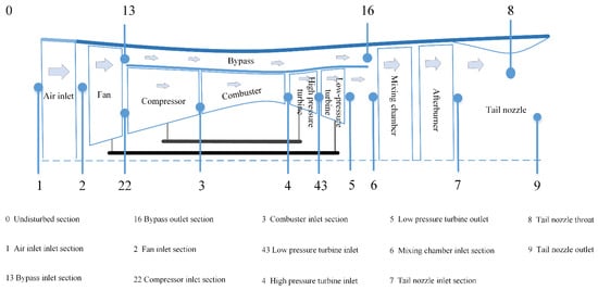
Figure 1. The cross-sectional schematic diagram of a turbofan engine.

3.1. The Structure of Aero-Engine Control System

The standard reinforcement learning setting is an infinite-horizon discounted Markov decision process (MDP), defined by a tuple $\left(\mathcal{S},\mathcal{A},\mathcal{P},r,{\rho }_0,\gamma \right)$, where $\mathcal{S}$ is the set of states, $\mathcal{A}$ the set of actions, $\mathcal{P}:\mathcal{S}\times \mathcal{A}\times \mathcal{S}\to ℝ$ the transition dynamic probability distribution, $r:\mathcal{S}\to ℝ$ the reward function, ${\rho }_0:\mathcal{S}\to ℝ$ the probability distribution of the initial state $s_0$, and $\gamma \in \left(0,1\right]$ the discounted factor determining the priority of short-term rewards. In reinforcement learning, an agent interacts with the environment and learns the reward-maximizing behavior, which is denoted as $\pi$. The policy $\pi$ maps the states to a probability distribution over the actions, i.e., $\pi :\mathcal{S}\times \mathcal{A}\to ℝ$.

The process of the agent learning in the interaction with the environment is shown in Figure 2. After the agent performs a certain action $a_t$, the environment will switch to a new state $s_{t+1}$, and the environment will generate a reward signal $r_t$ according to the new state. Subsequently, the agent executes a new action $a_{t+1}$ according to a certain policy $\pi$ and environmental feedback $s_{t+1}$. In this paper, the agent is the aero-engine controller, and the environment is the aero-engine that performs the acceleration process. Every time the controller interacts with the aero-engine, a tuple $\left(s_t,a_t,r_t,s_{t+1}\right)$ is generated and stored in the replay buffer, which will provide training sample support to optimize the policy $\pi$.

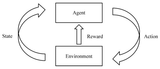
Figure 2. Reinforcement learning.

Figure 3 shows the structure of the aero-engine control system. The agent adopts the actor-critic framework, in which the actor is responsible for performing the action according to a certain policy while the critic is responsible for evaluating the quality of the action by outputting the advantage function. This process will be explained in detail in Section 4. The input of the actor is the state $s_t={\left[o_t,u_{t-1},o_{t-1},\dots ,u_{t-m+1},o_{t-m+1}\right]}^{\mathrm{T}}$, where $m$ is the depth of the trajectory and $o_t$ the observation of the environment at time $t$. If $m$ takes a larger value, which means that the current trajectory will have a longer influence of on the future. In the following simulation, the trajectory depth is selected as m = 2. The observation $o_t$ includes the states of the aero-engine $x_t$, the control error $e_t$, and the flight conditions $H,Ma$:

$$o_t={\left[x_t^{\mathrm{T}},e_t^{\mathrm{T}},H,Ma\right]}^{\mathrm{T}}$$

(2)

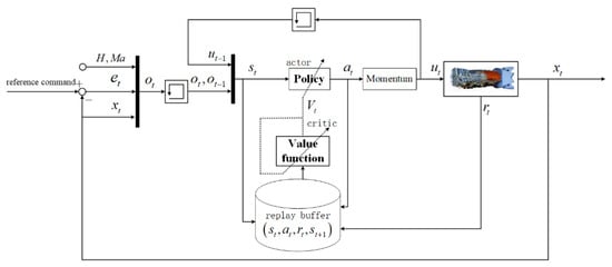
Figure 3. The aero-engine control system with deep reinforcement learning.

The state of the aero-engine is selected as $x={\left[N_{\mathrm{c},\mathrm{cor}},EPR,N_{\mathrm{f}},N_{\mathrm{c}},S_{\mathrm{mc}},S_{\mathrm{mf}},T_6\right]}^{\mathrm{T}}$, where $N_{\mathrm{c},\mathrm{cor}}$ is the corrected compressor rotor speed, $EPR$ is the engine pressure ratio, $N_{\mathrm{f}}$ is the physical fan rotor speed, $N_{\mathrm{c}}$ is the physical compressor rotor speed, $S_{\mathrm{mc}}$ is the compressor surge margin, $S_{\mathrm{mf}}$ is the fan surge margin, and $T_6$ is the high-pressure turbine outlet temperature. After the aero-engine executes the control variable vector $u_t$, the aero-engine state will shift from $x_t$ to $x_{t+1}$, and the aero-engine will output a reward signal $r_t$. The tuple $\left(s_t,a_t,r_t,s_{t+1}\right)$ constitutes a training sample, stored in the replay buffer.

3.2. Formulation of the Reward Signal

The reward $r_t$ is a very crucial signal, which is fed back to the critic from the aero-engine and contains information about the task goal. The process of formulating the reward is equivalent to the process of formulating learning goals for the agent.

The control objective is to minimize the error $e_t=\left[N_{\mathrm{c},\mathrm{cor},\mathrm{r}}-N_{\mathrm{c},\mathrm{cor},t},EP{R}_{\mathrm{r}}-EP{R}_t\right]$ between the controlled variables $\left[N_{\mathrm{c},\mathrm{cor},t},EP{R}_t\right]$ and the reference instructions $\left[N_{\mathrm{c},\mathrm{cor},\mathrm{r}},EP{R}_{\mathrm{r}}\right]$ by adjusting the input of the aero-engine $u_t=\left[W_{\mathrm{fb},\mathrm{cor},t},A_{8,t}\right]$ under different flight conditions. Due to the extreme operating environment of the aero-engines, it is necessary to ensure that the key performance parameters do not exceed the limit, including $N_{\mathrm{c}}$, $N_{\mathrm{f}}$, $S_{\mathrm{mc}}$, $S_{\mathrm{mf}}$, and $T_6$.

Based on the control objective, the reward signal can be defined as follows:

$$r_t=-p{e}_t^{\mathrm{T}}{e}_t-{{\displaystyle {\sum }_i{w}_i\left[\max \left(c_i\left(t\right)-c_{i,\mathrm{l}}\left(t\right),0\right)\right]}}^2$$

(3)

where $p$ and $w_i$ are the positive gain coefficients, $c_i\left(t\right)$ is a key performance parameter, and $c_{i,\mathrm{l}}\left(t\right)$ is the limit of the corresponding key performance parameter. The first error term $\mathrm{p}{e}_t^{\mathrm{T}}{e}_t$ on the right side of Equation (3) can ensure the tracking performance of the controller. The role of the second term on the right side of Equation (3) is to achieve restrictive protection. When the key performance parameters do not exceed the limit margin $c_i\left(t\right)\le c_{i,\mathrm{l}}\left(t\right)$, this term is equal to zero, so the control policy will not be affected when the key performance parameters do not exceed the limit. However, when the key performance parameters exceed the limit, the second term will give the agent a large negative benefit, which will drive the agent to avoid making a decision that will cause the over-limit problem.

3.3. The Structure of the Agent

As mentioned in Section 3.1, the agent is composed of the actor and the critic. The actor is a deep neural network to approximate the policy $\pi$, as shown in Figure 4. In the learning process, the agent needs to explore all the schemes in the feasible region to find the optimal policy without falling into the local optimum. Therefore, the policy learned by the actor would have some randomness. In Figure 4, the actor does not directly output the action $a_t$, but outputs the relevant parameters of the probability distribution of the action value. The normal distribution is adopted in this paper to approximate the probability distribution of the action, that is, the actor outputs the mean $\mu$ and variance $\sigma$ of the normal distribution $a_t\sim N\left(\mu ,\sigma \right)$.

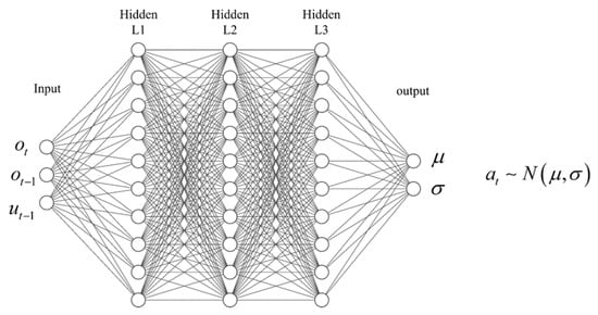
Figure 4. The structure of the actor neural network.

To prevent serious accidents such as surges and stalls caused by the randomness of the actions, a momentum term is introduced to suppress abrupt changes in the engine input, as shown in Figure 3 as follows:

$$u_t=\left(1-\epsilon \right)u_{t-1}+\epsilon a_t$$

(4)

where $\epsilon \in \left[0,1\right]$ is the momentum factor and $u_t$ the input of the aero-engine. In this way, even if $a_t$ changes abruptly, the input $u$ can remain stable when $\epsilon$ is much less than 1.

Similar to the actor, the critic is also a deep neural network the difference is that its output is the approximate state value function $V\left(s|\nu \right)$, where $\nu$ is the parameter vector of the critic network. The definition and use of $V\left(s|\nu \right)$ will be explained in Section 4.

4. Parameters Update of Actor-Critic Based on Deep Reinforcement Learning

Let $\eta \left(\pi \right)$ denote the expected discounted cumulative reward of the policy $\pi$:

$$\eta \left(\pi \right)={\mathbb{E}}_{s_0,a_0,\dots }\left({\displaystyle \sum _{t=0}^{\infty }{\gamma }^{t}r\left(s_t\right)}\right)$$

(5)

where $s_0\sim {\rho }_0\left(s_0\right)$, $a_t\sim \pi \left(a_t|s_t\right)$, $s_{t+1}\sim \mathcal{P}\left(s_{t+1}|s_t,a_t\right)$.

The aim of the agent is to learn the optimal policy ${\pi }^{\ast }$ to maximize the expected discounted cumulative rewards $\eta \left({\pi }^{\ast }\right)$. The state value function $V_{\pi }\left(s\right)$ and the action value function $Q_{\pi }\left(s,a\right)$ are defined as follows:

$$\begin{array}{c}{V}_{\pi }\left(s_t\right)={\mathbb{E}}_{a_t,s_{t+1},a_{t+1},\dots }\left({\displaystyle \sum _{k=0}^{\infty }{\gamma }^{k}r\left(s_{t+k}\right)}\right)\\ Q_{\pi }\left(s_t,a_t\right)={\mathbb{E}}_{s_{t+1},a_{t+1},\dots }\left({\displaystyle \sum _{k=0}^{\infty }{\gamma }^{k}r\left(s_{t+k}\right)}\right)\end{array}$$

(6)

where $a_t\sim \pi \left(a_t|s_t\right)$ and $s_{t+1}\sim \mathcal{P}\left(s_{t+1}|s_t,a_t\right)$.

It can be inferred from the Equation (6) that the state value function is the expectation of the action value function: $V_{\pi }\left(s_t\right)={\mathbb{E}}_{a_t\sim \pi }\left(Q_{\pi }\left(s_t,a_t\right)\right)$. The advantage function is defined as follows:

$$A_{\pi }\left(s_t,a_t\right)=Q_{\pi }\left(s_t,a_t\right)-V_{\pi }\left(s_t\right)$$

(7)

which indicates the advantage of the action $a_t$ under the state $s_t$. Ref. [21] has proved that the gap between the two expected discounted cumulative rewards $\eta \left(\pi \right)$ and $\eta \left(\tilde{\pi }\right)$ can be represented by the advantage function as follows:

$$\eta \left(\tilde{\pi }\right)=\eta \left(\pi \right)+{\mathbb{E}}_{s_0,a_0,s_1,a_1,\dots }\left({\displaystyle \sum _{t=0}^{\infty }{\gamma }^t{A}_{\pi }\left(s_t,a_t\right)}\right)$$

(8)

where $s_0\sim {\rho }_0\left(s_0\right)$, $a_t\sim \tilde{\pi }\left(a_t|s_t\right)$, $s_{t+1}\sim \mathcal{P}\left(s_{t+1}|s_t,a_t\right)$.

The second term on the right side of the Equation (8) can be expanded to the following:

$$\eta \left(\tilde{\pi }\right)=\eta \left(\pi \right)+{\displaystyle \sum _{t=0}^{\infty }{\gamma }^t{\displaystyle \sum _s{P}_{\tilde{\pi }}\left(s_t=s\right){\displaystyle \sum _a\tilde{\pi }\left(a_t=a|s_t\right)A_{\pi }\left(s_t,a_t=a\right)}}}$$

(9)

where $P_{\tilde{\pi }}\left(s_t=s\right)$ means the probability the state is $s_t$ at time $t$ when the actions are chosen according to policy $\tilde{\pi }$.

Define ${\rho }_{\pi }\left(s\right)={\displaystyle \sum _{t=0}^{\infty }{\gamma }^t{P}_{\pi }\left(s_t=s\right)}$. Equation (9) can be simplified to the following:

$$\eta \left(\tilde{\pi }\right)=\eta \left(\pi \right)+{\displaystyle \sum _s{\rho }_{\tilde{\pi }}\left(s\right)}{\displaystyle \sum _a\tilde{\pi }\left(a|s\right)}{A}_{\pi }\left(s,a\right)$$

(10)

Equation (9) implies a policy optimization method by maximizing the second term ${\displaystyle \sum _s{\rho }_{\tilde{\pi }}\left(s\right)}{\displaystyle \sum _a\tilde{\pi }\left(a|s\right)}{A}_{\pi }\left(s,a\right)$. If the policy parameterized, i.e.,${\pi }_{\theta }\left(a|s\right)$ is a differentiable function of the parameter vector $\theta$, the parameter update law can be constructed as follows:

$${\theta }_{i+1}={\theta }_i+\alpha {\nabla }_{\theta }\left({\displaystyle \sum _s{\rho }_{\tilde{\pi }}\left(s\right)}{\displaystyle \sum _a\tilde{\pi }\left(a|s\right)}{A}_{\pi }\left(s,a\right)\right)$$

(11)

where $\alpha$ is the update step size.

However, due to the complex dependency of ${\rho }_{\tilde{\pi }}\left(s\right)$ on $\tilde{\pi }$, it is impractical to optimize the policy with Equation (11) directly. A simple way to avoid this problem is to introduce a local approximation is as follows:

$$L_{\pi }\left(\tilde{\pi }\right)=\eta \left(\pi \right)+{\displaystyle \sum _s{\rho }_{\pi }\left(s\right)}{\displaystyle \sum _a\tilde{\pi }\left(a|s\right)}{A}_{\pi }\left(s,a\right)$$

(12)

where ${\rho }_{\tilde{\pi }}\left(s\right)$ is replaced by ${\rho }_{\pi }\left(s\right)$. $L_{\pi }$ matches $\eta \left(\pi \right)$ to first order. It means that for any ${\theta }_0$, there is the following:

$$\begin{array}{c}{L}_{{\pi }_{{\theta }_0}}\left({\pi }_{{\theta }_0}\right)=\eta \left({\pi }_{{\theta }_0}\right)\\ {\nabla }_{\theta }{L}_{{\pi }_{{\theta }_0}}\left({\pi }_{\theta }\right){|}_{\theta ={\theta }_0}={\nabla }_{\theta }\eta \left({\pi }_{\theta }\right){|}_{\theta ={\theta }_0}\end{array}$$

(13)

Equation (13) implies that a sufficiently small step that updates the policy ${\pi }_{{\theta }_0}\to \tilde{\pi }$ and increases $L_{{\pi }_{{\theta }_0}}$ will also lead to an increase in $\eta$. However, there is no guidance on how small the step size is to meet the requirements.

Ref. [22] has proved the following:

$$\eta \left(\tilde{\pi }\right)\ge L_{\pi }\left(\tilde{\pi }\right)-C{D}_{\mathrm{KL}}^{\max }\left(\pi ,\tilde{\pi }\right)$$

(14)

where $C=\frac{2\gamma {\max }_s{\max }_a\left|A_{\pi }\left(s,a\right)\right|}{{\left(1-\gamma \right)}^2}$, $D_{\mathrm{KL}}^{\max }\left(\pi ,\tilde{\pi }\right)=\underset{s}{\max }{D}_{\mathrm{KL}}\left[\pi \left(\cdot |s\right)\left|\right|\tilde{\pi }\left(\cdot |s\right)\right]$, and $D_{\mathrm{KL}}\left(\pi \left(\cdot |s\right)\left|\right|\tilde{\pi }\left(\cdot |s\right)\right)$ is the Kullback-Leibler Divergence.

Let

$$M_{\pi }\left(\tilde{\pi }\right)=L_{\pi }\left(\tilde{\pi }\right)-C{D}_{\mathrm{KL}}^{\max }\left(\pi ,\tilde{\pi }\right)$$

(15)

According to Equations (14) and (15), $\eta$ can be maximized by maximizing $M_{\pi }$, thus improving the policy.

The objective function needs to be transformed into an expectation representation so that it can be approximated using sampling-based methods, such as Monte Carlo simulation. Replace the sum over the actions with an importance sampling estimator the contribution of a single state $s$ to the objective function can be expressed as follows:

$${\displaystyle \sum _a{\pi }_{\theta }\left(a|s\right)A_{{\pi }_{{\theta }_0}}\left(s,a\right)={\mathbb{E}}_{a\sim q}\left[\frac{{\pi }_{\theta }\left(a|s\right)}{q\left(a|s\right)}{A}_{{\pi }_{{\theta }_0}}\left(s,a\right)\right]}$$

(16)

where $q\left(s,a\right)$ denotes the sampling distribution. In this paper, the training data are sampled according to the old policy ${\pi }_{{\theta }_0}$, so that $q\left(a|s\right)={\pi }_{{\theta }_0}\left(a|s\right)$. Further replace ${\displaystyle \sum _s{\rho }_{{\pi }_{{\theta }_0}}\left(s\right)}\left[\dots \right]$ with the expectation $E_{s\sim {\rho }_{{\pi }_{{\theta }_0}}}\left[\dots \right]$, the second term on the right side of Equation (12) is exactly equivalent to Equation (16), written in terms of expectations as follows:

$${\displaystyle \sum _s{\rho }_{{\pi }_{{\theta }_0}}\left(s\right)}{\displaystyle \sum _a{\pi }_{\theta }\left(a|s\right)}{A}_{{\pi }_{{\theta }_0}}\left(s,a\right)={\mathbb{E}}_{s\sim {\rho }_{{\pi }_{{\theta }_0}},a\sim {\pi }_{{\theta }_0}}\left[\frac{{\pi }_{\theta }\left(a|s\right)}{{\pi }_{{\theta }_0}\left(a|s\right)}{A}_{{\pi }_{{\theta }_0}}\left(s,a\right)\right]$$

(17)

The second term on the right side of Equation (15) $C{D}_{\mathrm{KL}}^{\max }\left(\pi ,\tilde{\pi }\right)$ is difficult to calculate. Actually, it can be regarded as a penalty item to reduce the update step size of the policy. In PPO, the objective is simplified to a form that is easier to implement the following:

$$J\left(\theta \right)={\mathbb{E}}_{s\sim {\rho }_{{\pi }_{{\theta }_0}},a\sim {\pi }_{{\theta }_0}}\left[\frac{{\pi }_{\theta }\left(a|s\right)}{{\pi }_{{\theta }_0}\left(a|s\right)}{A}_{{\pi }_{{\theta }_0}}\left(s,a\right)-\beta D_{\mathrm{KL}}\left[{\pi }_{{\theta }_0}\left(\cdot |s\right)\left|\right|{\pi }_{\theta }\left(\cdot |s\right)\right]\right]$$

(18)

where $\beta$ is an adaptive penalty coefficient, which will change with the average KL divergence ${\overline{D}}_{\mathrm{KL}}^{{\rho }_{{\pi }_{{\theta }_0}}}={\mathbb{E}}_{s\sim {\rho }_{{\pi }_{{\theta }_0}}}\left[D_{\mathrm{KL}}\left[{\pi }_{{\theta }_0}\left(\cdot |s\right)\left|\right|{\pi }_{\theta }\left(\cdot |s\right)\right]\right]$:

$$\beta \leftarrow \left\{\begin{array}{l}\beta /2 ,{\overline{D}}_{\mathrm{KL}}^{{\rho }_{{\pi }_{{\theta }_0}}}<D_{\mathrm{t}\arg }/\tau \\ \beta ,D_{\mathrm{t}\arg }/\tau \le {\overline{D}}_{\mathrm{KL}}^{{\rho }_{{\pi }_{{\theta }_0}}}<D_{\mathrm{t}\arg }\times \tau \\ \beta \times 2 ,{\overline{D}}_{\mathrm{KL}}^{{\rho }_{{\pi }_{{\theta }_0}}}>D_{\mathrm{t}\arg }\times \tau \end{array}\right.$$

where $\tau >1$ is a coefficient set heuristically, and $D_{\mathrm{t}\arg }$ the target value of the KL divergence. When ${\overline{D}}_{\mathrm{KL}}^{{\rho }_{{\pi }_{{\theta }_0}}}$ takes a small value, the adaptive coefficient $\beta$ will reduce the impact of the penalty term. Vice versa.

A critic neural network is built to estimate the state-value function $V_{\pi }\left(s|\nu \right)$, where $\nu$ is the parameter vector. $A_{{\pi }_{{\theta }_0}}\left(s,a\right)$ can be calculated through Equation (7), where $Q_{{\pi }_{{\theta }_0}}\left(s,a\right)$ can be approximated by $r\left(s,a\right)+\gamma V_{{\pi }_{{\theta }_0}}\left(s^{\prime }|\nu \right)$, $s^{\prime }\sim \mathcal{P}\left(s^{\prime }|s,a\right)$. Thus, Equation (18) can be updated to the following:

$$J\left(\theta \right)={\mathbb{E}}_{s\sim {\rho }_{{\pi }_{{\theta }_0}},a\sim {\pi }_{{\theta }_0}}\left[\frac{{\pi }_{\theta }\left(a|s\right)}{{\pi }_{{\theta }_0}\left(a|s\right)}{A}_{{\pi }_{{\theta }_0}}\left(s,a|\nu \right)-\beta D_{\mathrm{KL}}\left[{\pi }_{{\theta }_0}\left(\cdot |s\right)\left|\right|{\pi }_{\theta }\left(\cdot |s\right)\right]\right]$$

(19)

where $A_{{\pi }_{{\theta }_0}}\left(s,a|\nu \right)=r\left(s,a\right)+\gamma V_{{\pi }_{{\theta }_0}}\left(s^{\prime }|\nu \right)-V_{{\pi }_{{\theta }_0}}\left(s|\nu \right)$.

The aim of the critic neural network is to estimate the action-value function $Q$ accurately. With the insight of the Bellman function, its loss function can be designed as follows:

$$L\left(\nu \right)={\mathbb{E}}_{s\sim {\rho }_{{\pi }_{{\theta }_0}},a\sim {\pi }_{{\theta }_0},s^{\prime }\sim \mathcal{P}\left(s^{\prime }|s,a\right)}{\left[r\left(s,a\right)+\gamma V_{{\pi }_{{\theta }_0}}\left(s^{\prime }|\nu \right)-V_{{\pi }_{{\theta }_0}}\left(s|\nu \right)\right]}^2$$

(20)

The expectation in Equations (19) and (20), ${\mathbb{E}}_{s\sim {\rho }_{{\pi }_{{\theta }_0}},a\sim {\pi }_{{\theta }_0}}$ and ${\mathbb{E}}_{s\sim {\rho }_{{\pi }_{{\theta }_0}},a\sim {\pi }_{{\theta }_0},s^{\prime }\sim \mathcal{P}\left(s^{\prime }|s,a\right)}$, can be approximated by sampling from the replay buffer ${\mathbb{E}}_{\left(s,a,s^{\prime }\right)\sim \mathcal{R}}$, where $\mathcal{R}$ represents the replay buffer. According to $J\left(\theta \right)$, the parameter vector $\theta$ of the actor can be updated with the following gradient ascending method: $\theta \leftarrow \theta +\alpha {\nabla }_{\theta }J\left(\theta \right)$, while the parameter vector $\nu$ can be updated with the gradient descent method according to $L\left(\nu \right)$: $\nu \leftarrow \nu -\alpha {\nabla }_{\nu }L\left(\nu \right)$, where $\alpha$ is the learning rate.

5. Deep Neural Network Dynamic Prediction Model and Model-Based Reinforcement Learning

5.1. Deep Neural Network Dynamic Prediction Model

The tuple $\left(s,a,r,s^{\prime }\right)$ in the replay buffer contains the state transition information of the aero-engine, which can be used to train and identify the dynamic characteristics of the aero-engine. Therefore, a dynamic prediction model of the aero-engine based on a deep neural network is established in this section.

As shown in Figure 5, the recurrent neural network is selected as the network structure of the dynamic prediction model. The characteristic of the recurrent neural network is that the intermediate vector obtained by the operation of neurons at the last time can continue to be used as the input of neurons at the next time, which makes the relationship of input data in the time dimension reflect. The recurrent neural network can better mine a large amount of context information between training data and analyze the complex correlation between data in the time dimension. Moreover, the mechanism of recurrent neural network sharing parameter vectors for each time data can reduce the complexity of the model and the difficulty of training. As shown in Figure 5, the input layer transfers the network input, the state, and action vector pairs $\left[s,a\right]$, to the recurrent hidden layer. Through the loop connection on the recurrent hidden layer, the influence of times series samples in the future is retained, and the recurrent hidden layer vector $h$ is generated. Finally, the nonlinear ability is improved by the fully connected hidden layer, and the state prediction in the future ${\widehat{s}}^{\prime }$ is realized by the output layer. The forward propagation equation can be expressed as follows:

$$\begin{array}{c}{h}_t=\sigma \left(U{\left[s_t,a_t\right]}^{\mathrm{T}}+W{h}_{t-1}+b_1\right)\hfill \\ {\widehat{s}}_{t+1}=f_{\mathrm{full}}\left(V{h}_t+b_2\right)\hfill \end{array}$$

(21)

where $U$ is the weight matrix from the input layer to the recurrent hidden layer, $W$ is the weight matrix of the recurrent hidden layer connected in time dimension, $V$ is the weight matrix of the recurrent hidden layer to the fully connected hidden layer, while $b_1$ and $b_2$ are offset vectors, $\sigma$ is the activation function of the recurrent hidden layer, $f_{\mathrm{full}}$ is simplified to represent the whole fully connected hidden layer. ${\widehat{s}}_{t+1}$ predicted at time $t$ can be used as the network input at time $t+1$. According to the policy $a_{t+1}\sim \pi \left(\cdot |{\widehat{s}}_{t+1}\right)$, ${\widehat{s}}_{t+2}$ can be continuously predicted, and multi-step prediction can be realized by this cycle.

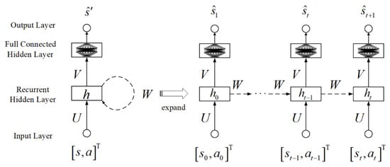
Figure 5. The network structure of the dynamic prediction model.

The tuples in the replay buffer are stored according to time to form a state-decision series chain $\left(s_0,a_0,s_1,a_1,\dots ,s_T,a_T\right)$, which is used as the training sample. The loss function related to the samples at time $t$ is the two norms of error vector between the real state $s_{t+1}$ and the predicted state ${\widehat{s}}_{t+1}$ at time $t+1$:

$${\mathcal{L}}_t={‖s_{t+1}-{\widehat{s}}_{t+1}‖}_2^2$$

(22)

While the overall loss function can be expressed as follows:

$${\mathcal{L}}_{l:T}={\displaystyle \sum _{t=l}^T{\mathcal{L}}_t}$$

(23)

where $l$ is defined as the prediction lag degree.

Finally, the gradient descent method is applied to train the network parameter vector according to the following overall loss function:

$$\varpi \leftarrow \varpi -\alpha {\nabla }_{\varpi }{\mathcal{L}}_{0:T}$$

(24)

For convenience, all the trainable parameters of the recurrent neural network are represented by parameter vector $\varpi$, including $V$, $W$, $U$, and the trainable parameters in $f_{\mathrm{full}}$.

5.2. Model-Based Method for Improving Training Efficiency

The algorithm mentioned in Section 4 is model-free, in which the transition dynamic probability distribution $\mathcal{P}$ is unnecessary. In Section 4, it is mentioned that the advantage function is calculated by the following:

$$\begin{array}{c}{A}_{{\pi }_{{\theta }_0}}\left(s_t,a_t|\nu \right)=Q_{{\pi }_{{\theta }_0}}\left(s_t,a_t\right)-V_{{\pi }_{{\theta }_0}}\left(s_t|\nu \right)\hfill \\ \hspace{1em}\hspace{1em}\hspace{1em}\hspace{1em}\hspace{1em}\hspace{1em}\approx r\left(s_t,a_t\right)+\gamma V_{{\pi }_{{\theta }_0}}\left(s^{\prime }|\nu \right)-V_{{\pi }_{{\theta }_0}}\left(s|\nu \right)\hfill \end{array}$$

where the action-value function $Q_{{\pi }_{{\theta }_0}}\left(s,a\right)$ is estimated by the following:

$$Q_{{\pi }_{{\theta }_0}}\left(s,a\right)\approx r\left(s,a\right)+\gamma V_{{\pi }_{{\theta }_0}}\left(s^{\prime }|\nu \right)$$

(25)

The first term $r\left(s,a\right)$ is the real value, while the second term $\gamma V_{{\pi }_{{\theta }_0}}\left(s^{\prime }|\nu \right)$ itself is an estimate, which will aggravate the estimation error of $Q_{{\pi }_{{\theta }_0}}\left(s,a\right)$. However, with the dynamic prediction model, the influence of $\gamma V_{{\pi }_{{\theta }_0}}\left(s^{\prime }|\nu \right)$ on the estimation error of $Q_{{\pi }_{{\theta }_0}}\left(s,a\right)$ can be weakened. Under the current state $s_t$ and action $a_t$, the prediction state-action pairs, ${\widehat{s}}_{t+1},{\widehat{a}}_{t+1},{\widehat{s}}_{t+2},{\widehat{a}}_{t+2},\dots ,{\widehat{s}}_{t+H},{\widehat{a}}_{t+H}$, can be obtained by multi-step prediction using the dynamic prediction model and policy, where $H$ is the prediction depth. According to the prediction state, the prediction reward function can be calculated: $\widehat{r}=r\left(\widehat{s},\widehat{a}\right)$.

The Equation (25) can thereby be replaced by the following:

$$Q_{{\pi }_{{\theta }_0}}\left(s_t,a_t\right)\approx Q_{{\pi }_{{\theta }_0}}^H\left(s_t,a_t|\nu \right)=r\left(s_t,a_t\right)+{\displaystyle \sum _{k=1}^H{\gamma }^{k}r\left({\widehat{s}}_{t+k},{\widehat{a}}_{t+k}\right)+{\gamma }^{H+1}{V}_{{\pi }_{{\theta }_0}}\left({\widehat{s}}_{t+H+1}|\nu \right)}$$

(26)

Because the discount factor $\gamma <1$, ${\gamma }^{H+1}$ becomes the key to reducing the influence of $V_{{\pi }_{{\theta }_0}}\left({\widehat{s}}_{t+H+1}|\nu \right)$. Although the prediction error $r-\widehat{r}$ in $H$ steps is introduced in, it also provides more information. From the empirical point of view, the convergence rate of the supervised learning of the dynamic prediction model is much faster than that of the reinforcement learning. Hence at the initial stage of the learning process, the addition of a dynamic prediction model can provide a more accurate estimation of the action value function $Q_{{\pi }_{{\theta }_0}}$, thus improving training efficiency of reinforcement learning.

Both Equations (19) and (20) can be improved to (27) and (28) with $Q_{{\pi }_{{\theta }_0}}^H$:

$$\begin{array}{c}J\left(\theta \right)={\mathbb{E}}_{s\sim {\rho }_{{\pi }_{{\theta }_0}},a\sim {\pi }_{{\theta }_0}}\left[\frac{{\pi }_{\theta }\left(a|s\right)}{{\pi }_{{\theta }_0}\left(a|s\right)}{A}_{{\pi }_{{\theta }_0}}\left(s,a|\nu \right)-\beta D_{\mathrm{KL}}\left[{\pi }_{{\theta }_0}\left(\cdot |s\right)\left|\right|{\pi }_{\theta }\left(\cdot |s\right)\right]\right]\\ A_{{\pi }_{{\theta }_0}}\left(s,a|\nu \right)=Q_{{\pi }_{{\theta }_0}}^H\left(s,a|\nu \right)-V_{{\pi }_{{\theta }_0}}\left(s|\nu \right)\end{array}$$

(27)

$$L\left(\nu \right)={\mathbb{E}}_{s\sim {\rho }_{{\pi }_{{\theta }_0}},a\sim {\pi }_{{\theta }_0},s^{\prime }\sim \mathcal{P}\left(s^{\prime }|s,a\right)}{\left[Q_{{\pi }_{{\theta }_0}}^H\left(s,a|\nu \right)-V_{{\pi }_{{\theta }_0}}\left(s|\nu \right)\right]}^2$$

(28)

This model-based reinforcement learning is summarized in Algorithm 1.

Algorithm 1

Initialize critic with $\nu$, actor with $\theta$, model network with $\varpi$, and replay buffer $\mathcal{R}$.

for $episode=1,2,\dots ,R$ do

Receive initial observation state $s_0\sim {\rho }_0$

for $t=0,1,\dots ,T$ do

$a_t\sim {\pi }_{{\theta }_0}\left(\cdot |s_t\right)$

$u_t=\epsilon a_t+\left(1-\epsilon \right)u_{t-1}$

Execute $u_t$ and observe reward $r_t$, and new states $s_{t+1}$.

Store transition $\left(s_t,a_t,r_t,s_{t+1}\right)$ in replay buffer

end for

Update $\varpi$ by minimizing the loss function with $k_1$ epochs

Update $\nu$ by minimizing the loss function with $k_2$ epochs

Update $\theta$ by maximizing the objective function with $k_3$ epochs

Initialize replay buffer

${\theta }_0\leftarrow \theta$

end for

6. Simulations and Analyses

In this paper, the digital simulation experiments are carried out based on the aero-engine component-level model. The control performance is verified by the acceleration task from the idle state to the intermediate state.

6.1. Hyperparameter Setting

There are some hyperparameters that need to be selected as follows to complete the simulation. The simulation step size is 0.02 s. The definitions and the values of some partial hyperparameters are listed in Table 1. The hyperparameters $\gamma$, $D_{\mathrm{t}\arg }$, $\tau$ are selected according to Ref. [22]. The momentum factor $\epsilon$ is introduced to prevent major accidents and model collapse in simulation, but too large a momentum factor will lead to too conservative a control algorithm. In the experiment, it is concluded that when $\epsilon$ is around 0.015, the model can run stably, and the influence on the control performance can be minimized. The key to the selection of hyperparameters $\mathrm{p}$ and ${\mathrm{w}}_i$ is that ${\mathrm{w}}_i$ is much larger than $\mathrm{p}$ to ensure the effect of limiting protection. In the experiment, the control policy of agent learning basically converges to the optimal policy within 2000 episodes, while the key parameters of the engine can be stable within 500 steps.

Table 1. Definitions and values of partial crucial hyperparameters.

Definition	Symbol	Value
Discounted factor	$\gamma$	0.99
Momentum factor	$\epsilon$	0.015
Gain coefficients of rewards	$\mathrm{p},{\mathrm{w}}_i$	100, 1000
Target value of the KL divergence	$D_{\mathrm{t}\arg }$	0.01
Threshold coefficient of target KL divergence	$\tau$	1.5
Maximum number of episodes	$R$	2000
Maximum number of simulation steps	$T$	500

The actor network has 3 fully connected hidden layers with 256, 256, and 256 units, respectively, while the critic network has 2 fully connected hidden layers with 256 and 256 units, respectively. The dynamic prediction model has a recurrent hidden layer and 2 fully connected hidden layers with 128 and 128 units, respectively. These three neural networks both use the rectified linear unit (ReLU) as the activation function for hidden layers, except that the output layer of the mean $\mu$ of the actor network is a tanh layer, the output layer of the variance $\sigma$ of the actor network is a sigmoid layer, and the recurrent layer of the dynamic prediction model is a tanh layer.

6.2. Performance of the DRL Controller

Since the essence of the DRL controller is a deep neural network estimator, estimation errors are inevitable. Such estimation errors have a great impact on the asymptotic performance of acceleration control. The steady-state error cannot be guaranteed to be zero, but it can be reduced to an acceptable range. The impact of the flight conditions on aero-engine performance is also a problem. The optimal policy learned by the agent should ensure satisfactory asymptotic performance under various flight conditions in the whole experimental flight envelope. Thousands of accelerated experiments are conducted, and training samples are collected to ensure that the trained agent learns the average optimal policy within the experimental flight envelope. Considering that the aero-engine acceleration process usually occurs at low altitudes and low Mach number, the flight conditions are set as $H\in \left[0km,\hspace{1em}4km\right]$, $Ma\in \left[0,\hspace{1em}0.5\right]$. The asymptotic performance in this paper is reflected by the steady-state error $e_{ss}=\left|\frac{N_{\mathrm{c},\mathrm{cor},\mathrm{r}}-N_{\mathrm{c}\_\mathrm{cor}}\left(\infty \right)}{N_{\mathrm{c},\mathrm{cor},\mathrm{r}}-N_{\mathrm{c}\_\mathrm{cor}}\left(t_0\right)}\right|+\left|\frac{EP{R}_{\mathrm{r}}-EPR\left(\infty \right)}{EP{R}_{\mathrm{r}}-EPR\left(t_0\right)}\right|$.

The steady-state errors in the flight envelope are shown in Figure 6. As can be seen from the results, the maximum steady-state error is 0.003542, and the average steady-state error is 0.001144, which is small enough to be negligible and will not affect aero-engine performance in practical applications.

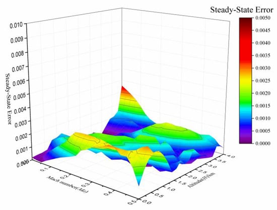
Figure 6. The steady-state error within the flight envelope.

This paper shows our controller’s dynamic performance of the complete acceleration task compared with the traditional PID controller with the min-max limit protection. The simulation results are shown in Figure 7, where the red solid lines represent the control curve of the DRL controller, the black solid lines represent the control curve of the traditional PID controller, the brown dot lines indicate the control reference instructions, and the yellow dash-dot lines indicate the limit boundary of key performance parameters. All variables in the Figure are normalized according to the design point parameters, so they are dimensionless.

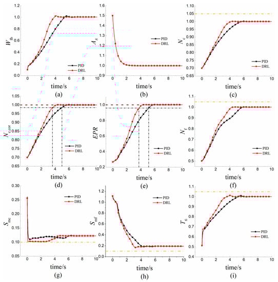
Figure 7. The acceleration process from the idle state to the intermediate state: (a) variation curve of the main fuel flow; (b) variation curve of the throat cross-sectional area; (c) response curve of the physical compressor rotor speed; (d) response curve of the corrected compressor rotor speed; (e) response curve of the engine pressure ratio; (f) response curve of the physical fan rotor speed; (g) response curve of the compressor surge margin; (h) response curve of the fan surge margin; (i) response curve of the high-pressure turbine outlet temperature.

As shown in Figure 7, the adjustment times of $N_{\mathrm{c},\mathrm{cor}}$ in the DRL controller and the PID controller are 3.62 s and 4.98 s, respectively, and the adjustment times of $EPR$ are 3.75 s and 4.98 s, respectively. The overshoots of $N_{\mathrm{c},\mathrm{cor}}$ and $EPR$ of the DRL controllers are 0.48% and 0.33%, respectively, while the overshoots of the PID controller are 0.5% and 0.5%, respectively. It can be seen from the figure that the acceleration process is mainly restricted by the surge margin of the compressor $S_{\mathrm{mc}}$. The $S_{\mathrm{mc}}$ of the DRL controller reaches the limit boundary at the first time and keeps close to it. Therefore, the dynamic process of the DRL controller’s acceleration task has reached the optimal performance under the condition of meeting the limit requirements, while the traditional PID controller is more conservative.

6.3. Performance of the Deep Neural Network Dynamic Prediction Model

This subsection will show the prediction accuracy of the dynamic prediction model from various aspects.

This subsection first focuses on the influence of the prediction lag degree on the prediction accuracy. As mentioned in Section 5.1, the training samples are multiple state-decision series chains $\left(s_0,a_0,s_1,a_1,\dots ,s_T,a_T\right)$ from time $0$ to $T$. The prediction starting time of the model is time $l$. Therefore, taking time $t$ as the prediction start time to predict ${\widehat{s}}_{t+1}$, at least $\left(s_{t-l},a_{t-l},s_{t-l+1},a_{t-l+1},\dots ,s_t,a_t\right)$ is needed. The relationship between the model prediction accuracy and the prediction lag degree is shown in Figure 8. The average value of the norm 1 of the state prediction error is applied to measure the model prediction accuracy as follows: $e_{s,1}={\displaystyle \sum _{i=1}^N\frac{{‖s_i-{\widehat{s}}_i‖}_1}{n}}$, where $N$ is the number of samples and $n$ the dimension of the state $s$. When the prediction lag degree $l=1$, $e_{s,1}=0.0228$ is the highest, while when $l=10$, $e_{s,1}=0.0045$ is the lowest. The figure shows that $e_{s,1}$ decreases roughly with the increase in the prediction lag degree $l$. However, in the case of a high prediction degree, the increase in $l$ has less and less influence on the model prediction accuracy. Because of the randomness, there may even be cases where the prediction lag is increased, but the prediction accuracy is reduced. In addition, the higher prediction lag degree means more computation in practical application. Therefore, it is necessary to make a balanced choice between the accuracy and the cost of computation. When the prediction lag degree is 4 or 5, the satisfactory prediction accuracy can be guaranteed with a low amount of computation.

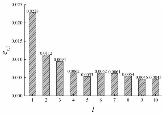
Figure 8. The relationship between the model prediction accuracy and the prediction lag degree.

The precondition of Equation (26) is to use the model to predict the future $H$-step state. Therefore, it is necessary to consider the error accumulation of multi-step rolling prediction. Figure 9 shows the relationship between the model prediction accuracy $e_{s,1}$ and the prediction depth $H$. When the prediction depth $H=1$, $e_{s,1}=0.0006$ is the lowest. With the increase in $H$, the prediction errors accumulated, but they all remained in the same order of magnitude, and all of them do not exceed 0.005. Therefore, the error accumulation of multi-step rolling prediction has negligible influence on the prediction accuracy.

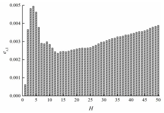
Figure 9. The relationship between the model prediction accuracy and the prediction depth.

Figure 10 compares the dynamic process simulation curves of the component-level model and the trained dynamic prediction model performing the same control task under the same control policy. Except for the same initial state, there is no data and information transmission between the component-level model, and the dynamic prediction model in the subsequent process. With the 2500 simulation steps, the prediction accuracy of the dynamic prediction model is not affected by error accumulation, and the whole simulation process has high prediction accuracy. Compared with the steady state process, the prediction accuracy of the transition state process is higher. The reason, we guess, is that the samples in the replay buffer are mostly transitional process data, which leads to more adequate training in fitting the transitional process. In Figure 10, the simulation curves of $EPR$, $S_{\mathrm{mf}}$, $T_6$ are partially enlarged. It can be clearly seen that the dynamic prediction model has a strong dynamic fitting ability, and even the slight vibration of the component-level model can be well reflected.

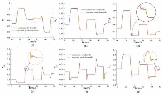
Figure 10. The comparison between the multi-step predictive control curve of the dynamic predictive model and the control curve of the component-level model: (a) simulation curve of the physical fan rotor speed; (b) simulation curve of the physical compressor rotor speed; (c) simulation curve of the engine pressure ratio; (d) simulation curve of the fan surge margin; (e) simulation curve of the compressor surge margin; (f) simulation curve of the high-pressure turbine outlet temperature.

6.4. Simulation Analysis of Model-Based Reinforcement Learning Method

The cumulative rewards of each episode in the learning process of the model-free and model-based methods are shown in Figure 11. The higher the reward, the better the control performance of the policy. Several simulation experiments are carried out to eliminate the influence of the randomness of the RL learning process. In Figure 11, the solid lines represent the average cumulative rewards in multiple experiments. The borders of the shadow region represent the maximum and minimum cumulative rewards in multiple experiments respectively. The blue part and the orange part represent the simulation results obtained from the model-based method and the model-free method, respectively. In the simulation episodes, the cumulative rewards of the two methods have an upward trend as a whole, which means that both methods can realize the optimization of the policy. The cumulative rewards of the model-free method and the model-based methods exceed −200 for the first time in the 250th episode and the 135th episode, respectively. At the beginning of the training process, the cumulative rewards have a downward trend, which is because the estimation of the value function is inaccurate, and the agent explores cluelessly. The agent in this period may output some dangerous actions. The model-based method can reduce the downward trend of the cumulative rewards in the early learning process. Consequently, compared with the model-free method, the model-based reinforcement learning method improved by using the dynamic prediction model can improve the learning efficiency, reduce the instability in the initial stage of learning, and realize the equivalent optimal policy faster.

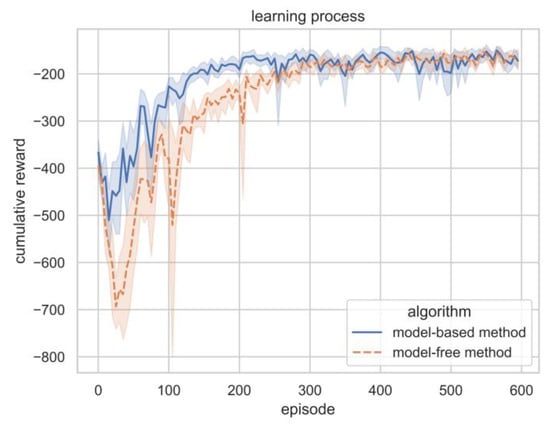
Figure 11. The cumulative rewards in learning process of model-free and model-based method.

7. Conclusions

This paper trains both the reinforcement learning controller and dynamic prediction model for the aero-engine. The proximal policy optimization algorithm is applied to train the controller, and the recurrent neural network is used as the structure of the dynamic prediction model.

The samples in the replay buffer of the reinforcement learning are used to train the dynamic prediction model, which in turn is used to improve the learning efficiency of reinforcement learning. Therefore, the combination of the two can obtain twice the result with half the effort.

The simulation results show that the deep reinforcement learning controller in this paper has satisfactory steady-state performance, and has a faster response speed than the traditional controller in the acceleration task from the idle state to the intermediate state. The dynamic prediction model itself has high prediction accuracy, and it can obviously improve the learning efficiency of reinforcement learning.

References

- Imani, A.; Montazeri-Gh, M. Improvement of Min–Max limit protection in aircraft engine control: An LMI approach. Aerosp. Sci. Technol. 2017, 68, 214–222. [Google Scholar] [CrossRef]
- Mnih, V.; Kavukcuoglu, K.; Silver, D.; Rusu, A.A.; Veness, J.; Bellemare, M.G.; Graves, A.; Riedmiller, M.; Fidjeland, A.K.; Ostrovski, G. Human-level control through deep reinforcement learning. Nature 2015, 518, 529–533. [Google Scholar] [CrossRef] [PubMed]
- Silver, D.; Lever, G.; Heess, N.; Degris, T.; Wierstra, D.; Riedmiller, M. Deterministic policy gradient algorithms. In Proceedings of the 31st International Conference on International Conference on Machine Learning, Beijing, China, 21–26 June 2014. [Google Scholar]
- Lillicrap, T.P.; Hunt, J.J.; Pritzel, A.; Heess, N.; Erez, T.; Tassa, Y.; Silver, D.; Wierstra, D. Continuous control with deep reinforcement learning. arXiv 2015, arXiv:1509.02971. [Google Scholar]
- Fujimoto, S.; Van Hoof, H.; Meger, D. Addressing function approximation error in actor-critic methods. arXiv 2018, arXiv:1802.09477. [Google Scholar]
- Barth-Maron, G.; Hoffman, M.W.; Budden, D.; Dabney, W.; Horgan, D.; Tb, D.; Muldal, A.; Heess, N.; Lillicrap, T. Distributed distributional deterministic policy gradients. arXiv 2018, arXiv:1804.08617. [Google Scholar]
- Gu, S.; Lillicrap, T.; Sutskever, I.; Levine, S. Continuous deep q-learning with model-based acceleration. In Proceedings of the International Conference on Machine Learning, New York, NY, USA, 19–24 June 2016; pp. 2829–2838. [Google Scholar]
- Schulman, J.; Wolski, F.; Dhariwal, P.; Radford, A.; Klimov, O. Proximal policy optimization algorithms. arXiv 2017, arXiv:1707.06347. [Google Scholar]
- Zheng, Q.; Jin, C.; Hu, Z.; Zhang, H. A study of aero-engine control method based on deep reinforcement learning. IEEE Access 2019, 7, 55285–55289. [Google Scholar] [CrossRef]
- Gu, S.; Holly, E.; Lillicrap, T.; Levine, S. Deep reinforcement learning for robotic manipulation with asynchronous off-policy updates. In Proceedings of the 2017 IEEE International Conference on Robotics and Automation (ICRA), Singapore, 29 May–3 June 2017; pp. 3389–3396. [Google Scholar]
- Xu, D.; Hui, Z.; Liu, Y.; Chen, G. Morphing control of a new bionic morphing UAV with deep reinforcement learning. Aerosp. Sci. Technol. 2019, 92, 232–243. [Google Scholar] [CrossRef]
- Liu, Y.; Liu, H.; Tian, Y.; Sun, C. Reinforcement learning based two-level control framework of UAV swarm for cooperative persistent surveillance in an unknown urban area. Aerosp. Sci. Technol. 2020, 98, 105671. [Google Scholar] [CrossRef]
- Ye, D.; Chen, G.; Zhang, W.; Chen, S.; Yuan, B.; Liu, B.; Chen, J.; Liu, Z.; Qiu, F.; Yu, H. Towards Playing Full MOBA Games with Deep Reinforcement Learning. In Proceedings of the 34th International Conference on Neural Information Processing Systems, Vancouver, BC, Canada, 6–12 December 2020; Volume 33. [Google Scholar]
- Feinberg, V.; Wan, A.; Stoica, I.; Jordan, M.I.; Gonzalez, J.E.; Levine, S. Model-based value estimation for efficient model-free reinforcement learning. arXiv 2018, arXiv:1803.00101. [Google Scholar]
- Buckman, J.; Hafner, D.; Tucker, G.; Brevdo, E.; Lee, H. Sample-efficient reinforcement learning with stochastic ensemble value expansion. In Proceedings of the 32nd International Conference on Neural Information Processing Systems, Red Hook, NY, USA; 2018; Volume 31, pp. 8224–8234. [Google Scholar]
- Kalweit, G.; Boedecker, J. Uncertainty-driven imagination for continuous deep reinforcement learning. In Proceedings of the Conference on Robot Learning, Mountain View, CA, USA; 2017; pp. 195–206. [Google Scholar]
- Kakade, S.; Langford, J. Approximately optimal approximate reinforcement learning. In Proceedings of the Nineteenth International Conference on Machine Learning, San Francisco, CA, USA, 8–12 July 2002; pp. 267–274. [Google Scholar]
- Schulman, J.; Levine, S.; Abbeel, P.; Jordan, M.; Moritz, P. Trust region policy optimization. In Proceedings of the International Conference on Machine Learning, Lille, France, 6–11 July 2015; pp. 1889–1897. [Google Scholar]
- Zheng, Q.; Fang, J.; Hu, Z.; Zhang, H. Aero-engine on-board model based on batch normalize deep neural network. IEEE Access 2019, 7, 54855–54862. [Google Scholar] [CrossRef]
- Zheng, Q.; Xi, Z.; Hu, C.; Zhang, H.; Hu, Z. A Research on Aero-engine Control Based on Deep Q Learning. Int. J. Turbo Jet-Engines 2022, 39, 541–547. [Google Scholar] [CrossRef]
- Yu, Z.; Lin, P.; Liu, L.; Zhu, C. A Control Method for Aero-engine Based on Reinforcement Learning. In Proceedings of the 2021 IEEE 4th International Conference on Big Data and Artificial Intelligence (BDAI), Qingdao, China, 2–4 July 2021; pp. 48–51. [Google Scholar]
- Qian, R.; Feng, Y.; Jiang, M.; Liu, L. Design and Realization of Intelligent Aero-engine DDPG Controller. J. Phys. Conf. Ser. 2022, 2195, 12056. [Google Scholar] [CrossRef]
- Singh, R.; Nataraj, P.; Maity, A. Nonlinear Control of a Gas Turbine Engine with Reinforcement Learning. In Proceedings of the Future Technologies Conference, Vancouver, BC, Canada, 28–29 October 2021; pp. 105–120. [Google Scholar]
- Hu, Q.; Zhao, Y. Aero-engine acceleration control using deep reinforcement learning with phase-based reward function. Proc. Inst. Mech. Eng. Part G J. Aerosp. Eng. 2022, 236, 1878–1894. [Google Scholar] [CrossRef]
- Gao, W.; Zhou, X.; Pan, M.; Zhou, W.; Lu, F.; Huang, J. Acceleration control strategy for aero-engines based on model-free deep reinforcement learning method. Aerosp. Sci. Technol. 2022, 120, 107248. [Google Scholar] [CrossRef]
- Tao, B.; Yang, L.; Wu, D.; Li, S.; Huang, Z.; Sun, X. Deep Reinforcement Learning-Based Optimal Control of Variable Cycle Engine Performance. In Proceedings of the 2022 International Conference on Advanced Robotics and Mechatronics (ICARM), Guilin, China, 3–5 July 2022; pp. 1002–1005. [Google Scholar]
- Zhu, Y.; Pan, M.; Zhou, W.; Huang, J. Intelligent direct thrust control for multivariable turbofan engine based on reinforcement and deep learning methods. Aerosp. Sci. Technol. 2022, 131, 107972. [Google Scholar] [CrossRef]
Disclaimer/Publisher’s Note: The statements, opinions and data contained in all publications are solely those of the individual author(s) and contributor(s) and not of MDPI and/or the editor(s). MDPI and/or the editor(s) disclaim responsibility for any injury to people or property resulting from any ideas, methods, instructions or products referred to in the content. |
© 2023 by the authors. Licensee MDPI, Basel, Switzerland. This article is an open access article distributed under the terms and conditions of the Creative Commons Attribution (CC BY) license (https://creativecommons.org/licenses/by/4.0/).