A Nonlinear Programming-Based Morphing Strategy for a Variable-Sweep Morphing Aircraft Aiming at Optimizing the Cruising Efficiency

Abstract

This work develops a morphing decision strategy to optimize the cruising efficiency for a variable-sweep morphing aircraft, and a simple and practical guidance and control system is given as well. They can work in tandem to accomplish a cruise mission effectively. To make the morphing decision accurately, we take into account the equilibrium equations of forces; the variations in airspeed, altitude, and mass and the optimal configurations for different cruise conditions are solved based on the nonlinear programming method with the objective of minimum engine thrust. Considering that a large amount of computational resources are required to solve the nonlinear programming problems, we establish an offline database of the optimal configurations and design a database-based online morphing decision process. In addition, the proposed morphing decision strategy includes an anti-disturbance mechanism, which ensures that the optimal configuration can be given accurately without chattering under fluctuating airspeed measurements. Comparative results from the simulations finally validate the effectiveness of the proposed strategy.

1. Introduction

Morphing aircraft can ensure optimal flight performance in different flight conditions by changing their shape [1]. Thus, such an aircraft has a larger flight envelope and better multi-mission capability than a fixed-geometry aircraft. However, historically, the increased weight and complexity caused by morphing mechanisms have limited the further development of morphing aircraft. In recent years, advances in aerospace materials and the pressure to expand the flight envelope have made morphing aircraft a hot research topic again [2,3,4,5,6].

Morphing brings parametric time-varying effects and additional control degrees of freedom, which pose a challenge to the design of flight control systems. In the current research on the control of morphing aircraft, most of the studies focus on the design of control laws to maintain the system’s stability and eliminate the time-varying effects and disturbances caused by morphing [7,8,9,10,11,12], for a predetermined morphing process. However, there are few works that regard morphing as a control input, and such works can be divided into two categories according to their objectives of morphing. The first category aims to minimize the tracking errors of the reference signals [13,14,15,16], and it usually requires adapting the methods of linearization and control allocation to model the aerodynamic coefficients as linear functions of the morphing parameters and to allocate control effects to each rudder surface and morphing mechanism. For instance, in [13], the aerodynamic coefficients are modeled as linear functions of wing telescopic proportions, and the sliding mode controller and control allocation method are employed to manipulate each control surface and telescopic wing. The second category aims to optimize the long-range performance of the morphing aircraft [17,18,19,20,21,22,23], which usually requires consideration of both control and optimization issues. It is clear that the optimal control method is a natural candidate [17,18]. However, the optimal control methods suffer from low flexibility and poor robustness, and they do not have the ability to make adjustments online. The scope of this paper belongs to the second category mentioned above; in more detail, it is to optimize the cruising efficiency for a variable-sweep morphing aircraft through morphing control. The morphing module should be designed with the capability to make morphing decisions to save fuel consumption and be able to coordinate with the guidance and control system of the morphing aircraft without violating the stability and flight performance.

The lift-to-drag ratio is an important parameter to determine cruising efficiency, and there have been some studies to design the morphing decision strategy with the objective of maximum lift-to-drag ratio. For instance, in [19], based on the multi-fidelity Kriging (MFK) model, the configurations with the maximum lift-to-drag ratio for different flight conditions are calculated, and the trajectory planning for optimal aerodynamic performance is performed. In [20], deep reinforcement learning is employed to determine the configuration with the largest lift-to-drag ratio to achieve the flight performance optimization of the morphing aircraft under different flight conditions. However, it should be noted that the cruise efficiency is not determined by the lift-to-drag ratio alone; this is because the fuel consumption depends on the magnitude of engine thrust, which is determined by the equations of forces balance and is not simply negatively related to the lift-to-drag ratio, but also related to altitude, aircraft mass, wind velocity, and many other factors. Currently, there still does not exist a study that can comprehensively take the above factors into account for the optimal morphing decision process of the morphing aircraft with the objective of minimum engine thrust. It is extremely important for the improvement of the cruise efficiency of the morphing aircraft to fill this gap. This was the main motive for this work.

In this paper, we first give the modeling of the inertial parameters and aerodynamic parameters of the variable-sweep morphing aircraft, then establish a 6-degree-of-freedom multi-loop cascaded morphing aircraft model, and design the flight guidance and control system based on the time-scale separation principle. Then, we establish an offline database of optimal configurations for different altitudes, Mach numbers, and aircraft masses based on nonlinear programming, and design a morphing decision process based on this offline database. The primary contributions and novelties of this paper are summarized in the following.

• Unlike previous works that aimed to optimize the lift-to-drag ratio [19,20], we optimize the engine thrust based on the force balance equations and take into account the cruise conditions at different altitudes, airspeeds, and levels of fuel reduction. Therefore, the proposed strategy can give a more accurate and reliable result for the optimal configuration.
• We take the wind effects and the measurement errors of the airspeed into account, and design a morphing decision process including an anti-disturbance mechanism, which can perform configuration optimization with fluctuating airspeed and avoid high frequency switching of the optimal configuration.
• The proposed morphing strategy was designed independently of the guidance and control system, which has high flexibility and can coordinate well with the guidance and control system to ensure the flight performance. Further, the morphing module, together with a six-degree-of-freedom cascaded morphing aircraft model and a guidance and control system, constitutes the closed-loop system (cf. Figure 1) for validating the effectiveness of the proposed morphing strategy, which contains fewer assumptions and can cover more mission scenarios.
  

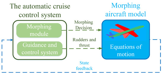  Figure 1. Closed-loop system consisting of morphing module, morphing aircraft model, and guidance and control system.

The rest of this paper is organized as follows. The variations in parameters due to morphing are presented in Section 2. The dynamic guidance and control of the morphing aircraft are described in Section 3. The morphing strategy design is depicted in Section 4. The comparative simulation studies are presented in Section 5, and the conclusion of this paper is given in Section 6.

2. Variations in Parameters Due to Morphing

The Firebee UAV [24] with the morphing concept proposed by NextGen Aeronautics [25] is used as the model of the variable-sweep morphing aircraft considered in this study. As shown in Figure 2, the shape and area of its wings vary significantly with the sweep angle $\zeta$, which ranges between 16 and 55 deg.

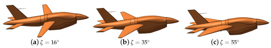
Figure 2. The configurations of the Firebee UAV.

2.1. Variations in Inertial Parameters

The inertial parameters, including static moment $\mathbf{S}$, the inertia matrix of the aircraft $\mathbf{J}$, wing area $S_{ref}$, mean aerodynamic chord $\overline{c}$, and wing span b, can be found in [8]. The values of these parameters at $\zeta ={16}^{°},{25}^{°},{35}^{°},{45}^{°},$ and ${55}^{°}$ are used to generate one-dimensional tables. Further, the values of these parameters can be interpolated from these tables. In this study, we should focus on the parameter $S_{ref}$, because it directly affects the magnitudes of lift and drag, which affect the cruising efficiency significantly.

According to Figure 3, as the sweep angle increases, $S_{ref}$ first increases, reaches a maximum at $\zeta ={45}^{°}$, and then decreases slightly. Note that both lift and drag increase linearly with $S_{ref}$ for the same angle of attack, but an increase in $S_{ref}$ also decreases the angle of attack of the aircraft in cruise conditions; this in turn leads to a decrease in drag. Therefore, there is a nonlinear relationship between $S_{ref}$ and the cruise efficiency of the aircraft.

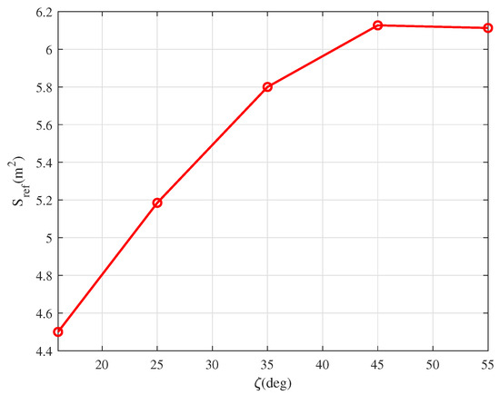
Figure 3. The variation in the $S_{ref}$ with respect to $\zeta$.

Remark 1.

In the subsequent optimization and simulation process, the inertial parameters are calculated based on the linear interpolation method. Another feasible method is the polynomial fitting method, and the difference between the results obtained by these two methods is very small.

2.2. Variation in Aerodynamic Parameters

Aerodynamic coefficients under different conditions—altitude h, airspeed V, angle of attack $\alpha$, and sweep angle $\zeta$—were obtained by DATCOM [26]. Considering the objective of optimizing cruise efficiency, we focus on the lift and drag coefficients that directly affect fuel consumption. To illustrate the aerodynamic performance under various airspeed and sweep angle conditions, the $C_L$, $C_D$, and $C_L/C_D$ under $h=7000\mathrm{m}$ are given in Figure 4, Figure 5 and Figure 6.

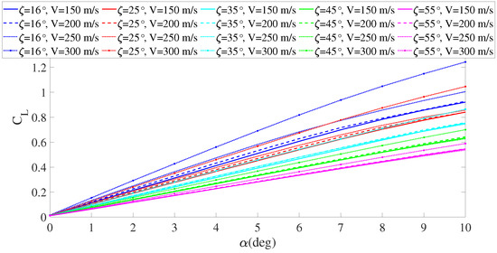
Figure 4. The lift coefficients $C_L$ for different conditions of V and $\zeta$ under $h=7000\mathrm{m}$.

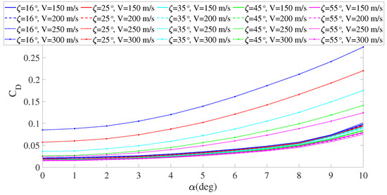
Figure 5. The drag coefficients $C_D$ for different conditions of V and $\zeta$ under $h=7000\mathrm{m}$.

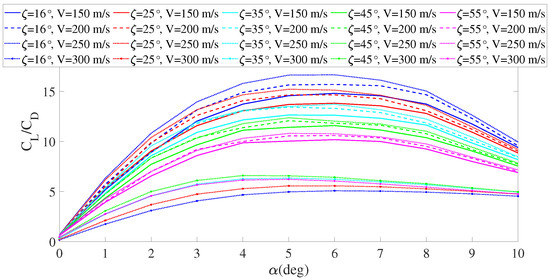
Figure 6. The lift-to-drag ratios $C_L/C_D$ for different conditions of V and $\zeta$ under $h=7000\mathrm{m}$.

It can be seen that the lift coefficient is positively correlated with the airspeed and negatively correlated with the sweep angle. Further, the drag coefficient is negatively correlated with the sweep angle $\zeta$, and it at first decreases with increasing airspeed, but as the airspeed approaches the transonic region ($V=300\mathrm{m}/\mathrm{s}$), the drag coefficient increases sharply, especially for the configurations with small sweep angles. Furthermore, when the airspeed does not reach the transonic region, the lift-to-drag ratio is negatively correlated with the sweep angle and positively correlated with the airspeed, whereas in the transonic region, the lift-to-drag ratio decreases sharply and is no longer negatively correlated with the sweep angle, and it can be observed that the configuration with $\zeta ={45}^{°}$ has the largest lift-to-drag ratio. To illustrate the effect of altitude on aerodynamic performance, the lift-to-drag ratios at different altitudes under $\alpha =2^{°}$ are given in Figure 7.

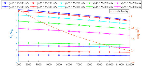
Figure 7. The variation in the $C_L/C_D$ with respect to altitude.

It can be seen in Figure 7 that the lift-to-drag ratio decreases slightly with increasing altitude. The variation in the air density with the altitude is more significant than that in the lift-drag ratio, and this relationship is estimated as $\rho \left(h\right)={\rho }_{0}exp(-h/h_s)$ [27], where ${\rho }_0=1.225$ is the nominal air density at sea level and $h_s^{-1}=9.43\times 10^{-5}$ is the air-density decay rate. Obviously, the variation in altitude causes changes in the aerodynamic coefficient and air density at the same time; among them, the latter has a more significant effect on the dynamic characteristics of the aircraft.

Remark 2.

In this study, we need to specify the flight state parameters such as altitude, Mach number, sweep angle, the position of the center of gravity, and the shape parameters of the aircraft’s fuselage and wings in the DATCOM input document. It should be noted that the wing shape parameters and center of gravity position vary with the sweep angle, and all the required parameters can be found in [8,24]. Further, we chose NASA-0010 as the airfoil section of the baseline aircraft and assumed that it does not change with morphing. In addition, we must admit that the DATCOM-based aerodynamic model may not be accurate, but it is sufficient to illustrate the morphing strategy presented in this paper, and the proposed morphing strategy can also be applied to the aerodynamic models built based on computational fluid dynamics (CFD) or wind tunnel tests without modification.

3. Dynamics, Guidance, and Control of the Morphing Aircraft

Based on the results in [24,28], we establish the equations of the motion as a cascade of the position loop, flight-path loop, attitude loop, and angular rate loop. Then, we give a guidance or control law for each loop; the guidance and control laws of all loops constitute the guidance and control system, which manipulates the rudders and engine thrust to accomplish cruise missions under shape-change conditions.

3.1. Dynamics of the Position Loop

3.1.1. Equations of the Motion of the Position Loop

The position of the aircraft is determined by longitude $\lambda$, latitude $\phi$, and altitude h, and the position state equations are

$$\begin{array}{c}\dot{h}=V_{e}sin\gamma ,\hfill \\ \dot{\lambda }=\frac{V_{e}cos\gamma cos\chi }{\left(a{\left(1-e^{2}sin\phi \right)}^{-\frac{1}{2}}+h\right)},\hfill \\ \dot{\phi }=\frac{V_{e}cos\gamma sin\chi }{\left[\left(a{\left(1-e^{2}sin\phi \right)}^{-\frac{1}{2}}+h\right)cos\phi \right]}.\hfill \end{array}$$

(1)

where $\gamma$ is the flight path angle; $\chi$ is the kinematic azimuth angle; and a and e are the semimajor axe and eccentricity of the Earth, respectively. $V_e$ is the ground speed of the aircraft, and it can be derived from the sum of the airspeed V and the wind velocity $V_w$ as

$$V_e=V+V_w.$$

(2)

3.1.2. Guidance Law of the Position Loop

To complete the cruise mission, the aircraft needs to reach the target waypoint $\left[{\lambda }_t,{\phi }_t,h_t\right]$; thus, we designed the guidance law for ${\gamma }_{des}$ and ${\chi }_{des}$ based on proportional-integral (PI) control and trigonometric methods, respectively. They can be formulated as follows:

$$\begin{array}{c}\begin{array}{c}{\gamma }_{des}=f_{sat}^{\gamma }\left(k_P^{\gamma }\left(h_t-h\right)+k_I^{\gamma }{I}_{e\gamma }\right),\hfill \\ {\dot{I}}_{e\gamma }=\left(h_t-h\right),\hfill \end{array}\\ {\chi }_{des}=\left\{\begin{array}{c}arccos\frac{-{\left({\phi }_t-\phi \right)}^2}{\sqrt{{\left({\lambda }_t-\lambda \right)}^2{cos}^2{\phi }_t+{\left({\phi }_t-\phi \right)}^2}},\left({\phi }_t-\phi \right)>0\hfill \\ arccos\frac{{\left({\phi }_t-\phi \right)}^2}{\sqrt{{\left({\lambda }_t-\lambda \right)}^2{cos}^2{\phi }_t+{\left({\phi }_t-\phi \right)}^2}},\left({\phi }_t-\phi \right)\le 0\hfill \end{array}\right..\end{array}$$

(3)

where $k_P^{\gamma }$ and $k_I^{\gamma }$ are the positive constants, $I_{e\gamma }$ is the output of the integrator, and $f_{sat}^{\gamma }$ is the saturation function for $\gamma$, which is defined as

$$f_{sat}^{\gamma }\left({\gamma }_d\right)=\left\{\begin{array}{c}{\gamma }_{max},{\gamma }_d\ge {\gamma }_{max}\hfill \\ {\gamma }_d,{\gamma }_{min}<{\gamma }_d<{\gamma }_{max}\hfill \\ {\gamma }_{min},{\gamma }_d\le {\gamma }_{min}\hfill \end{array}\right..$$

(4)

where ${\gamma }_d$ denotes the input variable of $f_{sat}^{\gamma }$; and ${\gamma }_{min}$ and ${\gamma }_{max}$ are the upper and lower bounds, respectively, of the amplitude constraint of ${\gamma }_{des}$.

3.2. Dynamics of the Flight-Path Loop

To clearly introduce the dynamics of the flight-path loop, the coordinate transformations among the flight-path coordinate system ${\mathrm{F}}_{\mathrm{H}}$, wind-axes coordinate system ${\mathrm{F}}_{\mathrm{V}}$, Earth-fixed coordinate system ${\mathrm{F}}_{\mathrm{I}}$, and body-fixed coordinate system ${\mathrm{F}}_{\mathrm{B}}$ are given in Figure 8.

Figure 8. The coordinate transformations between ${\mathrm{F}}_{\mathrm{H}}$, ${\mathrm{F}}_{\mathrm{V}}$, ${\mathrm{F}}_{\mathrm{I}}$, and ${\mathrm{F}}_{\mathrm{B}}$.

$u$ can be the position vector, velocity vector, or angular velocity vector of an arbitrary point, ${\mathbf{C}}_{\mathbf{BI}}$, ${\mathbf{C}}_{\mathbf{HI}}$, ${\mathbf{C}}_{\mathbf{VB}}$, and ${\mathbf{C}}_{\mathbf{HV}}$ are rotation matrices [29], and their expressions are given below.

$${\mathbf{C}}_{\mathbf{BI}}=\left[\begin{array}{ccc}cos\theta cos\psi & cos\theta sin\psi & -sin\theta \\ sin\varphi sin\theta cos\psi -cos\varphi sin\psi & sin\varphi sin\theta sin\psi +cos\varphi cos\psi & sin\varphi cos\theta \\ cos\varphi sin\theta cos\psi +sin\varphi sin\psi & cos\varphi sin\theta sin\psi -sin\varphi cos\psi & cos\varphi cos\theta \end{array}\right],$$

(5)

$${\mathbf{C}}_{\mathbf{VB}}=\left[\begin{array}{ccc}cos\alpha cos\beta & sin\beta & sin\alpha cos\beta \\ -cos\alpha sin\beta & cos\beta & -sin\alpha sin\beta \\ -sin\alpha & 0& cos\alpha \end{array}\right],$$

(6)

$${\mathbf{C}}_{\mathbf{IH}}=\left[\begin{array}{ccc}cos\chi cos\gamma & sin\chi cos\gamma & -sin\gamma \\ -sin\chi & cos\chi & 0\\ cos\chi sin\gamma & sin\chi sin\gamma & cos\gamma \end{array}\right],$$

(7)

$${\mathbf{C}}_{\mathbf{VH}}=\left[\begin{array}{ccc}1& 0& 0\\ 0& cos\mu & sin\mu \\ 0& -sin\mu & cos\mu \end{array}\right].$$

(8)

where $\psi$, $\theta$, and $\varphi$ denote the yaw, pitch, and roll angle, respectively; and $\alpha$, $\beta$, and $\mu$ are the angle of attack, slip, and back angle, respectively.

3.2.1. Equations of the Motion of the Flight-Path Loop

By ignoring the effect of the crosswind and applying Newton’s second law in the flight path coordinate system, the equations of motion can be obtained as

$$\left[\begin{array}{c}m{\dot{V}}_e\\ m{V}_{e}cos\gamma \dot{\chi }\\ -V\dot{\gamma }\end{array}\right]={\mathbf{C}}_{\mathbf{VH}}^{\mathbf{T}}{\mathbf{C}}_{\mathbf{VB}}\left(\left[\begin{array}{c}{f}_{\mathrm{ix}}\\ f_{\mathrm{iy}}\\ f_{\mathrm{iz}}\end{array}\right]+\left[\begin{array}{c}T\\ 0\\ 0\end{array}\right]\right)+{\mathbf{C}}_{\mathbf{VH}}^{\mathbf{T}}\left[\begin{array}{c}-D\\ 0\\ -L\end{array}\right]+{\mathbf{C}}_{\mathbf{HI}}\left[\begin{array}{c}0\\ 0\\ mg\end{array}\right].$$

(9)

where T is the engine thrust; $f_{ix}$, $f_{iy}$, and $f_{iz}$ are the components of inertia in $F_B$, and their expressions are given below [24].

$$\left[\begin{array}{c}{f}_{ix}\\ f_{iy}\\ f_{iz}\end{array}\right]=\left[\begin{array}{c}\dot{q}{S}_z-\dot{r}{S}_y+2\left(q{\dot{S}}_z-r{\dot{S}}_y\right)+q\left(p{S}_y-q{S}_x\right)-r\left(r{S}_x-p{S}_z\right)+{\ddot{S}}_x\\ \dot{r}{S}_x-\dot{p}{S}_z+2\left(r{\dot{S}}_x-p{\dot{S}}_z\right)+r\left(q{S}_z-r{S}_y\right)-p\left(p{S}_y-q{S}_x\right)+{\ddot{S}}_x\\ \dot{q}{S}_y-\dot{r}{S}_x+2\left(q{\dot{S}}_y-r{\dot{S}}_x\right)+q\left(r{S}_x-p{S}_z\right)-q\left(q{S}_z-p{S}_y\right)+{\ddot{S}}_z\end{array}\right].$$

(10)

where $S_x$, $S_y$, and $S_z$ are the components of the static moment on the x, y, and z axes of $F_B$, respectively. Further, D and L are drag and lift, and they can be formulated as

$$\begin{array}{c}D=\overline{q}{S}_{ref}\left(\zeta \right)\left(C_D^{{\alpha }^2}\left(\zeta ,V,h\right){\alpha }^2+C_D^{\alpha }\left(\zeta ,V,h\right)\alpha +C_D^0\left(\zeta ,V,h\right)\right),\hfill \\ L=\overline{q}{S}_{ref}\left(\zeta \right)\left(C_L^{\alpha }\left(\zeta ,V,h\right)\alpha +C_L^0\left(\zeta ,V,h\right)\right).\hfill \end{array}$$

(11)

where $\overline{q}=\frac{1}{2}\rho \left(h\right)V^2$ is the dynamic pressure.

3.2.2. Control Law of the Flight-Path Loop

The control objective of the flight-path loop is to steer V, $\chi$, and $\gamma$ to $V_{des}$, ${\chi }_{des}$, and ${\gamma }_{des}$ by properly designing $T_{des}$, ${\mu }_{des}$, and ${\alpha }_{des}$. Note that the dynamic characteristics of the flight-path loop are affected by the time-varying aerodynamic coefficients and additional inertial forces caused by morphing; thus, the designed control law should have good robustness. Considering the slow response of the signals in the flight-path loop, the PI control method is used to design the control law as

$$\begin{array}{c}{\mu }_{des}=f_{sat}^{\mu }\left(k_{\mu p}\left({\chi }_{des}-\chi \right)+k_{\mu I}{I}_{e\chi }\right),\hfill \\ {\dot{I}}_{e\chi }=\left({\chi }_{des}-\chi \right),\hfill \end{array}$$

(12)

$$\begin{array}{c}{\alpha }_{des}=f_{sat}^{\alpha }\left(k_{\alpha p}\left({\gamma }_{des}-\gamma \right)+k_{\alpha I}{I}_{e\gamma }\right),\hfill \\ {\dot{I}}_{e\gamma }=\left({\gamma }_{des}-\gamma \right),\hfill \end{array}$$

(13)

$$\begin{array}{c}{T}_{des}=f_{sat}^T(k_{vp}\left(V_r-V\right)+k_{vI}{I}_{ev}),\hfill \\ {\dot{I}}_{ev}=\left(V_r-V\right).\hfill \end{array}$$

(14)

where $k_{\mu p}$, $k_{\mu I}$, $k_{\alpha p}$, $k_{\alpha I}$, $k_{vp}$, and $k_{vI}$ are the positive constants. Further, $I_{e\chi }$, $I_{e\gamma }$, and $I_{ev}$ are the outputs of the integrators. Furthermore, $f_{sat}^{\mu }$, $f_{sat}^{\alpha }$, and $f_{sat}^T$ are the saturation functions for the $\gamma$, $\alpha$, and T, respectively. Their definitions are given below.

$$f_{sat}^{\mu }\left({\mu }_d\right)=\left\{\begin{array}{c}{\mu }_{max},{\mu }_d\ge {\mu }_{max}\hfill \\ {\mu }_d,{\mu }_{min}<{\mu }_d<{\mu }_{max}\hfill \\ {\mu }_{min},{\mu }_d\le {\mu }_{min}\hfill \end{array}\right.,$$

(15)

$$f_{sat}^{\alpha }\left({\alpha }_d\right)=\left\{\begin{array}{c}{\alpha }_{max},{\alpha }_d\ge {\alpha }_{max}\hfill \\ {\alpha }_d,{\alpha }_{min}<{\alpha }_d<{\alpha }_{max}\hfill \\ {\alpha }_{min},{\alpha }_d\le {\alpha }_{min}\hfill \end{array}\right.,$$

(16)

$$f_{sat}^T\left(T_d\right)=\left\{\begin{array}{c}{T}_{max},T_d\ge T_{max}\hfill \\ T_d,T_{min}<T_d<T_{max}\hfill \\ T_{min},T_d\le T_{min}\hfill \end{array}\right..$$

(17)

where ${\mu }_d$, ${\alpha }_d$, and $T_d$ denote the input variables of the saturation functions. Further, ${\mu }_{min}$, ${\alpha }_{min}$, and $T_{min}$ are the lower bounds of ${\mu }_{des}$, ${\alpha }_{des}$, and $T_{des}$, respectively. Furthermore, ${\mu }_{max}$, ${\alpha }_{max}$, and $T_{max}$ are the upper bounds of ${\mu }_{des}$, ${\alpha }_{des}$, and $T_{des}$, respectively.

3.3. Dynamics of the Attitude Loop

3.3.1. Equations of the Motion of the Attitude Loop

The equations of motion in the attitude loop are the same as those for a fixed-geometry aircraft, and they can be described as

$$\left[\begin{array}{c}\dot{\mu }\\ \dot{\alpha }\\ \dot{\beta }\end{array}\right]={\left[\begin{array}{ccc}cos\alpha cos\beta & 0& sin\alpha \\ sin\beta & 1& 0\\ sin\alpha cos\beta & 0& -cos\alpha \end{array}\right]}^{-1}\left({\mathbf{C}}_{\mathbf{VB}}^{\mathbf{T}}{\mathbf{C}}_{\mathbf{VH}}\left[\begin{array}{c}-\dot{\chi }sin\gamma \\ \dot{\gamma }\\ \dot{\chi }cos\gamma \end{array}\right]+\left[\begin{array}{c}p\\ q\\ r\end{array}\right]\right).$$

(18)

where p, q, and r, denote the roll, pitch, and yaw rate components of the aircraft angular velocity vector in ${\mathrm{F}}_{\mathrm{B}}$, respectively.

3.3.2. Control Law of the Attitude Loop

The control law for the attitude loop should steer $\mu$, $\alpha$, and $\beta$ to ${\mu }_{des}$, ${\alpha }_{des}$, and ${\beta }_{des}$ by properly designing $p_{des}$, $q_{des}$, and $r_{des}$. Note that the dynamics of the attitude loop have strong nonlinearity, but there are no external disturbances and model uncertainties; thus, we designed ${\left[\begin{array}{ccc}{p}_{des}& q_{des}& r_{des}\end{array}\right]}^{\mathrm{T}}$ based on nonlinear dynamic method [30] as Equation (19) and Figure 9.

$$\begin{gathered} \begin{array}{c}\begin{array}{c}\left[\begin{array}{c}{p}_{des}\\ q_{des}\\ r_{des}\end{array}\right]=\left[\begin{array}{ccc}cos\alpha cos\beta & 0& sin\alpha \\ sin\beta & 1& 0\\ sin\alpha cos\beta & 0& -cos\alpha \end{array}\right]\left[\begin{array}{c}{k}_{\mu p}({\mu }_{des}-\mu )+k_{\mu I}{I}_{e\mu }\\ k_{\alpha p}({\alpha }_{des}-\alpha )+k_{\alpha I}{I}_{e\alpha }\\ k_{\beta p}({\beta }_{des}-\beta )+k_{\beta I}{I}_{e\beta }\end{array}\right]\hfill \\ +{\mathbf{C}}_{\mathbf{VB}}^{\mathbf{T}}{\mathbf{C}}_{\mathbf{VH}}\left[\begin{array}{c}-\dot{\chi }sin\gamma \\ \dot{\gamma }\\ \dot{\chi }cos\gamma \end{array}\right],\hfill \end{array}\end{array} \\ {\dot{I}}_{e\mu }=({\mu }_{des}-\mu ), \\ {\dot{I}}_{e\alpha }=({\alpha }_{des}-\alpha ), \\ {\dot{I}}_{e\beta }=({\beta }_{des}-\beta ). \end{gathered}$$

(19)

where $k_{\mu p}$, $k_{\mu I}$, $k_{\alpha p}$, $k_{\alpha I}$, $k_{\beta p}$, and $k_{\beta I}$ are the positive design parameters. Further, $I_{e\mu }$, $I_{e\alpha }$, and $I_{e\beta }$ are the outputs of the integrators.

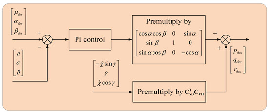
Figure 9. The control block diagram of the attitude loop.

3.4. Dynamics of the Angular Rate Loop

3.4.1. Equations of the Motion of the Angular Rate Loop

By applying the angular momentum theorem in the body-fixed coordinate system, the equations of motion can be obtained as

$$\left[\begin{array}{c}\dot{p}\\ \dot{q}\\ \dot{r}\end{array}\right]={\mathit{J}}^{-1}\left(\left[\begin{array}{c}{l}_a+l_g+l_i\\ m_a+m_g+m_i\\ n_a+n_g+n_i\end{array}\right]-\left[\begin{array}{c}p\\ q\\ r\end{array}\right]\times \mathit{J}\left[\begin{array}{c}p\\ q\\ r\end{array}\right]\right),$$

(20)

where $\mathit{J}$ is the inertia matrix of the aircraft, and

$$\left[\begin{array}{c}{l}_a\\ m_a\\ n_a\end{array}\right]=\left[\begin{array}{c}{C}_{l\beta }\beta +C_{lp}\frac{pb}{2V}+C_{lr}\frac{rb}{2V}+C_{l{\delta }_a}{\delta }_a+C_{l{\delta }_r}{\delta }_r\\ C_{m0}+C_{m\alpha }\alpha +C_{mq}\frac{q\overline{c}}{2V}+C_{m{\delta }_e}{\delta }_e\\ C_{n\beta }\beta +C_{np}\frac{pb}{2V}+C_{nr}\frac{rb}{2V}+C_{n{\delta }_a}{\delta }_a+C_{n{\delta }_r}{\delta }_r\end{array}\right]$$

(21)

is the array of the components of aerodynamic moments in $F_b$. $C_{l\beta }$, $C_{lp}$, $C_{lr}$, $C_{l{\delta }_a}$, $C_{l{\delta }_r}$, $C_{m0}$, $C_{m\alpha }$, $C_{mq}$, $C_{m{\delta }_e}$, $C_{n\beta }$, $C_{np}$, $C_{nr}$, $C_{n{\delta }_a}$, and $C_{n{\delta }_r}$ are all the aerodynamic moment coefficients. Further,

$$\left[\begin{array}{c}{l}_g\\ m_g\\ n_g\end{array}\right]=\left[\begin{array}{c}{S}_x\\ S_y\\ S_z\end{array}\right]\times \left({\mathbf{C}}_{\mathbf{B}/\mathbf{I}}\left[\begin{array}{c}0\\ 0\\ mg\end{array}\right]\right)$$

(22)

is the array of the components of moment caused by gravity in $F_b$. ${\left[\begin{array}{ccc}{l}_i& m_i& n_i\end{array}\right]}^{\mathrm{T}}$ is the array of components of the moment caused by the movement of the centroid, and its expression is given below [24].

$$\begin{array}{c}\left[\begin{array}{c}{l}_i\\ m_i\\ n_i\end{array}\right]=\left[\begin{array}{c}{S}_x\\ S_y\\ S_z\end{array}\right]\times \dot{\mathit{v}}+\left[\begin{array}{c}{S}_x\\ S_y\\ S_z\end{array}\right]\times \left(\left[\begin{array}{c}p\\ q\\ r\end{array}\right]\times \mathit{v}\right)\hfill \\ -2\int {\mathit{\rho }}_{\mathit{i}}\times \left({\mathit{\rho }}_{\mathit{i}}\times \left[\begin{array}{c}p\\ q\\ r\end{array}\right]\right)d{m}_i+\int {\mathit{\rho }}_{\mathit{i}}\times {\ddot{\mathit{\rho }}}_{\mathit{i}}d{m}_i\hfill \end{array}$$

(23)

where $\mathit{v}={\mathit{C}}_{\mathit{V}\mathit{B}}^{\mathrm{T}}{\left[\begin{array}{ccc}V& 0& 0\end{array}\right]}^{\mathrm{T}}$ denotes the components of the array of the ground speed in $F_b$, and ${\mathit{\rho }}_{\mathit{i}}={\left[\begin{array}{ccc}{\rho }_{xi}& {\rho }_{yi}& {\rho }_{zi}\end{array}\right]}^{\mathrm{T}}$ is the position vector relative to the origin of $F_b$ of each particle in the whole aircraft.

3.4.2. Control Laws for the Angular Rate Loop

The control objective for altitude loop is to steer p, q, and r to $p_{des}$, $q_{des}$, and $r_{des}$ by properly designing ${\delta }_a$, ${\delta }_e$, and ${\delta }_r$. It should be noted that the signals in the angular rate loop change rapidly, and the change in shape brings time-varying effects and disturbances. Therefore, the incremental dynamic inversion method [31] is employed to design ${\left[\begin{array}{ccc}{\delta }_a& {\delta }_e& {\delta }_r\end{array}\right]}^{\mathrm{T}}$, which is given below:

$$\begin{array}{c}\left[\begin{array}{c}\Delta {\delta }_a\\ \Delta {\delta }_e\\ \Delta {\delta }_r\end{array}\right]={\mathit{J}}^{-1}\overline{q}{S}_{ref}\left[\begin{array}{ccc}{C}_{l{\delta }_a}& 0& C_{l{\delta }_r}\\ 0& C_{m{\delta }_e}& 0\\ C_{n{\delta }_a}& 0& C_{l{\delta }_n}\end{array}\right]\hfill \\ \left(\left[\begin{array}{c}{k}_{pp}(p_{des}-p)+k_{pI}{I}_{ep}\\ k_{qp}(q_{des}-q)+k_{qI}{I}_{eq}\\ k_{rp}(r_{des}-r)+k_{rI}{I}_{er}\end{array}\right]-\left[\begin{array}{c}{\dot{p}}_0\\ {\dot{q}}_0\\ {\dot{r}}_0\end{array}\right]\right),\hfill \\ \left[\begin{array}{c}{\delta }_a\\ {\delta }_e\\ {\delta }_r\end{array}\right]=\left[\begin{array}{c}{\delta }_{a0}\\ {\delta }_{e0}\\ {\delta }_{r0}\end{array}\right]+\left[\begin{array}{c}\Delta {\delta }_a\\ \Delta {\delta }_e\\ \Delta {\delta }_r\end{array}\right],\hfill \\ {\dot{I}}_{ep}=p_{des}-p,I_{ep}\left(0\right)=0,\hfill \\ {\dot{I}}_{eq}=q_{des}-q,I_{eq}\left(0\right)=0,\hfill \\ {\dot{I}}_{er}=r_{des}-r,I_{er}\left(0\right)=0.\hfill \end{array}$$

(24)

where $k_{pp}$, $k_{pI}$, $k_{qp}$, $k_{qI}$, $k_{rp}$, and $k_{rI}$ are positive design parameters; $I_{ep}$, $I_{eq}$, and $I_{er}$ are the outputs of the integrators. $p_0$, $q_0$, $r_0$, ${\dot{p}}_0$, ${\dot{q}}_0$, ${\dot{r}}_0$, ${\delta }_{a0}$, ${\delta }_{e0}$, and ${\delta }_{r0}$ are the values of p, q, r, $\dot{p}$, $\dot{q}$, $\dot{r}$, ${\delta }_a$, ${\delta }_e$, and ${\delta }_r$, respectively, in the last control cycle as

$$\begin{array}{c}{p}_0\left(t\right)=p\left(t-d_{ct}\right),\hfill \\ q_0\left(t\right)=q\left(t-d_{ct}\right),\hfill \\ r_0\left(t\right)=r\left(t-d_{ct}\right),\hfill \\ {\delta }_{a0}\left(t\right)={\delta }_a\left(t-d_{ct}\right),\hfill \\ {\delta }_{e0}\left(t\right)={\delta }_e\left(t-d_{ct}\right),\hfill \\ {\delta }_{r0}\left(t\right)={\delta }_r\left(t-d_{ct}\right),\hfill \\ {\dot{p}}_0\left(t\right)=\dot{p}\left(t-d_{ct}\right),\hfill \\ {\dot{q}}_0\left(t\right)=\dot{q}\left(t-d_{ct}\right),\hfill \\ {\dot{r}}_0\left(t\right)=\dot{r}\left(t-d_{ct}\right).\hfill \end{array}$$

(25)

where $d_{ct}$ is the control cycle of the guidance and control system.

To make the control structure clearer and more understandable, the overall control block diagram of the angular rate loop is shown in Figure 10.

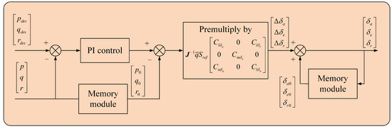
Figure 10. The control block diagram of the angular rate loop.

3.5. Dynamics of the Morphing Mechanism and Fuel Consumption

Note that the response speeds of the morphing mechanism and the engine thrust are relatively slow; thus, we model their dynamics as follows.

The actuator dynamic the morphing mechanism is modeled as a first-order dynamic system as below.

$$\dot{\zeta }=\frac{\left({\zeta }_{des}-\zeta \right)}{{\tau }_m}.$$

(26)

where ${\zeta }_{des}$ is the commanded sweep angle, $\zeta$ is the actual sweep angle, and ${\tau }_m$ is the inertia time constant of the morphing mechanism. Considering that the response speed of the morphing mechanism is much slower than that of the rudder surface (the time constant of the rudder surface is about 1/20), we set ${\tau }_m$ to 1/1.6 in this study.

Considering the hysteresis effect of fuel on the engine thrust response as a first-order dynamic system as well, we establish the following fuel consumption model.

$$\begin{array}{c}\dot{T}=\frac{\left(T_{des}-T\right)}{{\tau }_T},\hfill \\ \dot{m}=-IT.\hfill \end{array}$$

(27)

where $T_{des}$ is the commanded thrust given by the guidance and control system, T is the actual engine thrust, I is the specific impulse of the engine, and ${\tau }_T$ is the inertial time constant of the engine. By referring to some open sources and the literature [24], ${\tau }_T$ was set to 1/5.

Remark 3.

To avoid unnecessary complexity, there are some reasonable simplifications in the equations of motion of the morphing aircraft. We regard the Earth as a standard ellipsoid and neglect the effect of the Earth’s rotation. In addition, the effect of crosswind is neglected, i.e., we only consider the component of the wind in the x axis of the wind-axes coordinate system.

Remark 4.

The guidance and control system of a morphing aircraft should have stronger robustness and better environmental adaptability than that of a fixed-geometry aircraft. This is because it needs to ensure high flight performance in multiple configurations and system stability during the morphing process. The guidance and control laws given in this paper were designed based on this principle, and they can be replaced by better performance guidance and control laws that satisfy the same conditions.

4. Morphing Strategy Design

4.1. Off-Line Configuration Optimization

From Equation (27), it is clear that the objective of optimizing the cruising efficiency implies minimizing the engine thrust. In the cruising state, the thrust of the aircraft should satisfy the following equations of force balance.

$$\begin{array}{c}L-mg+Tsin\alpha =0,\hfill \\ D-Tcos\alpha =0.\hfill \end{array}$$

(28)

According to Equations (11) and (28), the value of T can be jointly determined by V, h, m, $\zeta$, and $\alpha$; among them, V, h, and m are obtained according to the cruising conditions, and $\zeta$ and $\alpha$ are set as decision variables. Then, we can construct a nonlinear optimization problem with the objective of minimizing the engine thrust as given below.

$$\begin{array}{c}{J}^{\ast }\left(V,h,m\right)=\underset{\zeta ,\alpha }{min}\frac{C_D\left(\zeta ,V,h,\alpha \right)}{cos\alpha },\hfill \\ subjecttoL-mg=\frac{tan\alpha }{2}\rho \left(h\right)V^2{S}_w\left(\zeta \right)C_D\left(\zeta ,V,h,\alpha \right),\hfill \\ {16}^{°}\le \zeta \le {55}^{°},\hfill \\ 0^{°}\le \alpha \le {10}^{°}.\hfill \end{array}$$

(29)

Remark 5.

In this study, since the specific impulse of the engine is assumed to be a constant, the optimization aiming at the minimum fuel consumption is exactly equivalent to the optimization aiming at the minimum T. In the real world, the specific impulse is affected by various factors (incoming pressure, temperature, etc.), and in fact, such matters are of less importance in the current investigation.

To save computational resources, we established a database of the optimal ${\zeta }^{\ast }$ with respect to V, h, and m by offline computation. We set the values of V, h, and m according to a three-dimensional grid. In the first dimension, we set the minimum value of V to 100 m/s, the maximum value to 300 m/s, and the value interval to 5 m/s; in the second dimension, we set the minimum value of h to 3000 m, the maximum value to 12,000 m, and the value interval to 500 m; in the third dimension, we set the minimum value of m to 750 kg, the maximum value to 1300 kg, and the value interval to 50 kg.

For each grid point i contained in the three-dimensional grid, the NPSOL [32] toolbox was applied to solve the nonlinear optimization problem, Equation (29), to get the optimal configuration ${\zeta }^{\ast i}$ and record it. We sliced the optimization results according to h and show the filled contour plot of the optimal configuration in Figure 11.

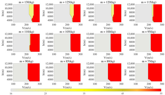
Figure 11. Filled contour plot of the optimal configuration.

Remark 6.

NPSOL is a popular nonlinear programming solver which uses sequential quadratic programming, with a positive-definite quasi-Newton approximation of the transformed Hessian of the Lagrangian function. All functionalities of the NPSOL solvers are available and changeable in the tomlab toolbox [33]. In addition, to ensure that the solver can find the optimal solution satisfying the constraint, we can change the initial solution vector several times and judge the convergence of the solution based on the output of the solver until a converged optimal solution is found. Such an approach reflects the advantage of offline computing, i.e., allowing a larger amount of computation and a certain degree of manual intervention.

As can be seen in Figure 11, the sweep angles of the optimal configurations take values of $\zeta ={16}^{°}$, ${25}^{°}$, and ${55}^{°}$ under $m\ge 110\mathrm{kg}$; and the optimal sweep angle only takes values of $\zeta ={16}^{°}$ and ${55}^{°}$ under $m<110\mathrm{kg}$. Further, it is clear that the optimal sweep angle is $\zeta ={16}^{°}$ at low airspeeds, and as airspeed increases, it switches to ${55}^{°}$, or first to ${25}^{°}$ and finally to ${55}^{°}$. Furthermore, with the increasing of altitude and decreasing of mass, ${\zeta }^{\ast }$ tends to increase—i.e., the area of the large sweep angle region increases in the filled contour map.

Remark 7.

It is worth noting that the optimal configuration of the morphing aircraft model used in this paper only takes values of $\zeta ={16}^{°}$, ${25}^{°}$, and ${55}^{°}$. Therefore, by substituting these values into Equation (28), the cruising thrust of each configuration can be solved, and the optimal configuration can be obtained directly by comparing the obtained thrust values, which greatly simplifies the computation. However, this method can only be applied to the Firebee UAV model used in this paper, whereas the nonlinear programming-based method proposed in this subsection can be easily extended to other morphing aircraft models.

4.2. Online Morphing Decision Process

Based on the established offline database, the nearest neighbor interpolation is used to determine the optimal configurations for different cruise conditions online. The Euclidean distance from the current operating state $[V,h,m]$ to each grid point is calculated as

$$d_p^i=\sqrt{{\left(V-V^i\right)}^2+{\left(h-h_{}^i\right)}^2+{\left(m-m_{}^i\right)}^2}.$$

(30)

where $\left[V^i,h^i,m^i\right]$ is the coordinate of the i-th grid point. Then, we find the grid point with the smallest $d_p^i$ and take its ${\zeta }^{\ast i}$ as the optimal configuration ${\zeta }^{\ast }$.

It should be noted that the airspeed during the cruise is affected by the wind velocity, and there are errors in the sensor measurements of airspeed. Consequently, the measured airspeed of the aircraft is a fluctuating value, which may cause the ${\zeta }^{\ast }$ to switch back and forth between several configurations, thereby compromising the stability and flight performance of the aircraft. To solve this problem, we must design a proper morphing decision process that contains an anti-disturbance mechanism to ensure the configuration optimization can be accomplished and the high-frequency switching does not occur under fluctuating airspeed measurement.

We first introduce a scoring mechanism to evaluate the score of each configuration. The offline computation was again adopted to establish a database of the scores of the configurations. For each grid point of the three-dimensional grid, by substituting $\zeta ={16}^{°},$${25}^{°},{35}^{°},{45}^{°},$ and ${55}^{°}$ into the Equation (28), the engine thrust levels $T_{16}^i$, $T_{25}^i$, $T_{35}^i$, $T_{45}^i$, and $T_{55}^i$ can be derived, and they were recorded as the baseline scores for $\zeta ={16}^{°},{25}^{°},{35}^{°},{45}^{°},$ and ${55}^{°}$. Therefore, we could derive a score database consisting of the baseline scores for each grid point. Further, the scores for the configuration with $\zeta \in \left[{16}^{°},{55}^{°}\right]$ were obtained by the linear interpolation method online.

For each control cycle, the difference between the scores of the current optimization result ${\zeta }^{\ast }\left(t\right)$ and the output of the previous time step ${\zeta }_{des}(t-d_{ct})$ is used to measure the degree of the urgency of the morphing action ${\zeta }^{\ast }\left(t\right)$. If this difference is greater than a threshold value $t_{hr}$, ${\zeta }^{\ast }\left(t\right)$ should be performed immediately; otherwise, the action should be executed based on the delayed action, rule as given below.

$$\begin{array}{c}{\zeta }_{des}\left(t\right)=\left\{\begin{array}{c}{\zeta }^{\ast }\left(t\right),ifcount\left(t\right)\ge N\hfill \\ {\zeta }_p\left(t\right),ifcount\left(t\right)<N\hfill \end{array}\right.,\hfill \\ {\zeta }_p\left(t\right)=\left\{\begin{array}{c}{\zeta }_p\left(t-d_{ct}\right),if{\zeta }^{\ast }\left(t\right)-{\zeta }^{\ast }\left(t-d_{ct}\right)<\Delta \zeta \hfill \\ {\zeta }^{\ast }\left(t\right),if{\zeta }^{\ast }\left(t\right)-{\zeta }^{\ast }\left(t-d_{ct}\right)\ge \Delta \zeta \hfill \end{array}\right.,\hfill \\ count\left(t\right)=\left\{\begin{array}{c}count\left(t-d_{ct}\right)+1,if({\zeta }^{\ast }\left(t\right)-{\zeta }^{\ast }\left(t-d_{ct}\right)<\Delta \zeta )\hfill \\ and(count\left(t\right)<N)\hfill \\ 1,{\zeta }^{\ast }\left(t\right)-{\zeta }^{\ast }\left(t-d_{ct}\right)>\Delta \zeta ,if({\zeta }^{\ast }\left(t\right)-{\zeta }^{\ast }\left(t-d_{ct}\right)\ge \Delta \zeta \hfill \\ or(count\left(t\right)\ge N)\hfill \end{array}\right.,\hfill \\ {\zeta }_{des}\left(0\right)=\zeta \left(0\right),\hfill \\ {\zeta }_p\left(t\right)=\zeta \left(0\right),\hfill \\ count\left(0\right)=1.\hfill \end{array}$$

(31)

where ${\zeta }_p$ is the memorized optimization result of the timer, $count$ is the timing’s variable, $\Delta \zeta$ is the threshold value for timer reset, and N is the number of delayed time steps.

Finally, we summarize the workflow of the proposed database-based online morphing decision process as follows (Algorithm 1):

Algorithm 1: Database-based online morphing decision process

Parameters:  threshold value for timer reset $\Delta \zeta$, threshold value for the difference of scores $t_{hr}$, control cycle $d_{ct}$, the number of delayed time steps N.

1:                     Initialize $t=0$, $count=1$, ${\zeta }_{des}\left(0\right)=\zeta \left(0\right)$, ${\zeta }_p\left(0\right)=\zeta \left(0\right)$.

2:                     $t=t+d_{ct}$

3:                     while cruise mission not over do

4:                        Calculate the Euclidean distance from the current state $[V,h,m]$ to each grid point according to Equation (30), and find the grid point i with the smallest $d_p^i$. Then, select the optimal configuration ${\zeta }^{*}$ from the grid point i

5:                        Calculate the scores $S_c\left({\zeta }^{*}\left(t\right)\right)$ and $S_c\left({\zeta }_{des}\left(t-d_{ct}\right)\right)$ of ${\zeta }^{*}\left(t\right)$ and ${\zeta }_{des}\left(t-d_{ct}\right)$ by linear interpolation from $[T_{16}^i,T_{25}^i,T_{35}^i,T_{45}^i,T_{55}^i]$.

6:                         if $S_c\left({\zeta }^{*}\left(t\right)\right)-S_c\left({\zeta }_{des}\left(t-d_{ct}\right)\right)<t_{hr}$, then

7:                             if ${\zeta }^{*}\left(t\right)-{\zeta }^{*}\left(t-d_{ct}\right)<\Delta \zeta$, then

8:                                 $count=count+1$.

9:                             else

10:                                 $count=1.$

11:                                 ${\zeta }_p={\zeta }^{*}\left(t\right)$.

12:                             end if

13:                             if $count>N$ then

14:                                 ${\zeta }_{des}\left(t\right)={\zeta }^{*}\left(t\right)$

15:                                 ${\zeta }_p\left(t\right)={\zeta }^{*}\left(t\right).$

16:                                 $count=1$.

17:                             else

18:                                 ${\zeta }_p\left(t\right)={\zeta }_p\left(t-d_{ct}\right)$

19:                                 ${\zeta }_{des}\left(t\right)={\zeta }_p\left(t\right)$

20:                             end if

21:                         else

22:                             ${\zeta }_{des}\left(t\right)={\zeta }^{*}\left(t\right)$.

23:                             ${\zeta }_p\left(t\right)={\zeta }^{*}\left(t\right)$.

24:                             $count=1.$

25:                         end if

26:                         output ${\zeta }_{des}$ to morphing mechanism.

27:                         $t=t+d_{ct}$.

28:                     end while

Remark 8.

In algorithm 1, lines 7–20 describe the proposed delayed action rule, which are the detailed implementation steps of Equation (31). As it is shown, the output ${\zeta }_{des}$ of the morphing module becomes ${\zeta }^{\ast }$ if ${\zeta }^{\ast }$ can hold for N control cycles without any change beyond $\Delta \zeta$. Otherwise, ${\zeta }_{des}$ stays at the last morphing module’s output ${\zeta }_p$.

5. Simulation

In this section, comparative simulations are presented to demonstrate the performance and effctiveness of the proposed morphing strategy. The control cycle of the guidance and control system was set to $d_{ct}$ = 0.01 s. The specific impulse of the engine was set to I = 18,000 N·s/kg. The parameter settings of the guidance and control system and morphing module are listed in Table 1.

Table 1. The parameter settings of the guidance and control system and morphing module.

Name	Value	Name	Value	Name	Value
$k_{\chi p}$	4.5	$k_{\gamma p}$	3.5	$k_{vp}$	20,000
$k_{\mu p}$	4	$k_{\alpha p}$	18	$k_{\beta p}$	8
$k_{pp}$	20	$k_{qp}$	20	$k_{rp}$	20
$k_{\chi I}$	1	$k_{\gamma I}$	0.5	$k_{vI}$	200
$k_{\mu I}$	1	$k_{\alpha I}$	1	$k_{\beta I}$	1
$k_{pI}$	2	$k_{qI}$	2	$k_{rI}$	2
${\gamma }_{max}$	${60}^{°}$	${\mu }_{max}$	${60}^{°}$	${\alpha }_{max}$	${10}^{°}$
${\gamma }_{min}$	$-{60}^{°}$	${\mu }_{min}$	$-{60}^{°}$	${\alpha }_{min}$	$-5^{°}$
$T_{max}$	$\mathrm{10,000}\mathrm{N}$	$\Delta \zeta$	$1^{°}$	$t_{hr}$	30
$T_{min}$	$500\mathrm{N}$	${\beta }_{des}$	$0^{°}$	N	200

Remark 9.

In Table 1, the parameters in rows 1–6 are the gains of the guidance and control system, which were determined by trial and error to ensure good flight performance under multiple configurations and flight conditions. Considering that the aircraft should maintain stable flight attitude during the cruise mission, we set the limitations of γ, α, μ, and T to relatively small ranges. Further, ${\beta }_{des}$ was set to zero to enable coordinated turns. Furthermore, the morphing module parameters $\Delta \zeta$, $t_{hr}$, and N were tuned based on trial and error and the numerical results of offline optimization.

5.1. Comparison with Fixed-Geometry Aircraft

In this subsection, the fuel consumption of the morphing aircraft with the proposed morphing strategy is compared with that of the fixed-geometry aircraft, which was taken to be the configuration of the Firebee UAV with $\zeta ={35}^{°}$. In addition, the extra weight brought by morphing mechanism was taken into account; the empty weight of the fixed-geometry aircraft was set to $90\%$ of that of the morphing aircraft. The cruise mission was to reach the waypoints sequentially at the specified velocity. The longitude, latitude, and cruise velocity of the waypoints are listed in Table 2, and the initial states of the morphing aircraft and the integrators were set as given in Table 3.

Table 2. Waypoint settings for Section 5.1.

Number	$\mathit{\phi }$	$\mathit{\lambda }$	h	${\mathit{V}}_{\mathit{e}}$
Point1	${50}^{°}$	${50}^{°}$	5000 m
Point2	${51}^{°}$	${50}^{°}$	5000 m	230 m/s
Point3	$53.5^{°}$	${50}^{°}$	7000 m	230 m/s
Point4	$53.5^{°}$	$51.5^{°}$	7000 m	180 m/s
Point5	$53.5^{°}$	$53.5^{°}$	6000 m	280 m/s

Table 3. Initial state settings of the morphing aircraft and the integrators in Section 5.1.

Name	Value	Name	Value	Name	Value
${\phi }_0$	${50}^{°}$	${\lambda }_0$	${50}^{°}$	$h_0$	5000 m
$V_0$	230 m/s	${\chi }_0$	$0^{°}$	${\gamma }_0$	$0^{°}$
${\mu }_0$	$0^{°}$	${\alpha }_0$	$0.73°$	${\beta }_0$	$0^{°}$
$p_0$	$0^{°}$/s	$q_0$	$0^{°}$/s	$r_0$	$0^{°}$/s
$I_{ev0}$	10	$I_{e\chi 0}$	0	$I_{e\gamma 0}$	0
$I_{e\mu 0}$	0	$I_{e\alpha 0}$	0	$I_{e\beta 0}$	0
$I_{ep0}$	0	$I_{eq0}$	0	$I_{er0}$	0
$T_0$	1430 N	$m_0$	$1250\mathrm{kg}$ (1175 kg for fixed-geometry aircraft)

According to Figure 12 and Figure 13, the morphing module selected a configuration with ${\zeta }_{des}={16}^{°}$ during the cruise between waypoints 1 and 2. Subsequently, during waypoints 2 and 3, the increase in altitude made the morphing module select a configuration with a larger sweep angle of ${\zeta }_{des}={25}^{°}$, and then the reduction in mass due to fuel consumption made the optimal sweep angle switch to ${\zeta }_{des}={55}^{°}$. Note that the cruise velocity during waypoints 3 and 4 will be lower, so the morphing mechanis m selected a configuration with ${\zeta }_{des}={16}^{°}$, and the morphing module selected a configuration with ${\zeta }_{des}={55}^{°}$ as the cruise velocity increased to 280 m/s between waypoints 4 and 5.

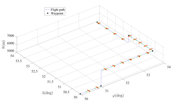
Figure 12. Flight path of the morphing aircraft with proposed morphing strategy in Section 5.1.

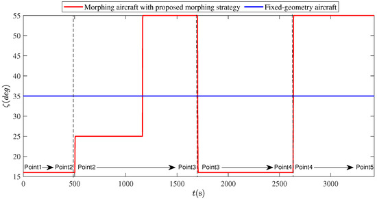
Figure 13. $\zeta$ of the comparative simulation in Section 5.1.

It can be concluded from Figure 14 and Figure 15 that despite the additional 75 kg added by the morphing mechanism, the fuel consumption of the morphing aircraft using the proposed morphing strategy is lower than that of the fixed-geometry aircraft in every cruise phase, especially in the high-speed cruise phase between waypoints 4 and 5. The fuel consumption of the morphing aircraft is 22.4% less than that of the fixed-geometry aircraft. In addition, between the waypoints 1 and 2, 2 and 3, and 3 and 4, the morphing aircraft using the proposed morphing strategy saved 1.89%, 2.16%, and 3.67% of fuel consumption, respectively, compared to the fixed-geometry aircraft.

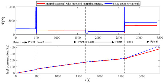
Figure 14. Engine thrust and fuel consumption of the comparative simulation in Section 5.1.

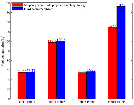
Figure 15. Fuel consumption for each cruise phase of the comparative simulation in Section 5.1.

As seen in Figure 16, the guidance and control system given in this paper can ensure the completion of the cruise mission, and all signals are always stable and bounded. Further, the morphing control module can work well with the guidance and control system and will not affect the stability and flight performance.

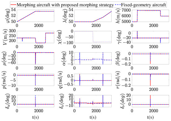
Figure 16. The states and rudder sufaces of the comparative simulation in Section 5.1.

5.2. Comparison with the Strategy Aiming at Optimizing the $C_L/C_D$

In this subsection, the proposed morphing strategy is compared with the morphing strategy aiming at optimizing the lift-to-drag ratio as in [19]. We set up the cruise mission as shown in Table 4, and the initial states of the morphing aircraft and the integrators as shown in Table 5.

Table 4. Waypoint settings in Section 5.2.

Number	$\mathit{\phi }$	$\mathit{\lambda }$	h	${\mathit{V}}_{\mathit{e}}$
Point1	${50}^{°}$	${50}^{°}$	6000 m
Point2	${50}^{°}$	${51}^{°}$	6000 m	210 m/s
Point3	$51.5^{°}$	${51}^{°}$	7000 m	230 m/s
Point4	${53}^{°}$	${51}^{°}$	7000 m	240 m/s
Point5	$53.5^{°}$	$52.5^{°}$	7000 m	270 m/s

Table 5. Initial state settings of the morphing aircraft and the integrators in Section 5.2.

Name	Value	Name	Value	Name	Value
${\phi }_0$	${50}^{°}$	${\lambda }_0$	${50}^{°}$	$h_0$	6000 m
$V_0$	210 m/s	${\chi }_0$	$0^{°}$	${\gamma }_0$	$0^{°}$
${\mu }_0$	$0^{°}$	${\alpha }_0$	$0.{73}^{°}$	${\beta }_0$	$0^{°}$
$p_0$	$0^{°}$/s	$q_0$	$0^{°}$/s	$r_0$	$0^{°}$/s
$I_{ev0}$	10	$I_{e\chi 0}$	0	$I_{e\gamma 0}$	0
$I_{e\mu 0}$	0	$I_{e\alpha 0}$	0	$I_{e\beta 0}$	0
$I_{ep0}$	0	$I_{eq0}$	0	$I_{er0}$	0
$T_0$	1430 N	$m_0$	$1250\mathrm{kg}$

It can be seen in Figure 17 and Figure 18 that the proposed morphing strategy first gives the morphing decision ${\zeta }_{des}={16}^{°}$, and then switches to ${\zeta }_{des}={25}^{°}$, and finally to ${\zeta }_{des}={55}^{°}$. It should be noted that there are significance differences between the decisions given by the proposed morphing strategy and the morphing strategy aiming at optimizing the $C_L/C_D$. Between waypoints 1 and 4, the morphing strategy aiming at optimizing the lift-to-drag ratio selected a configuration with ${\zeta }_{des}={16}^{°}$, whereas for cruising between waypoints 4 and 5, a configuration with ${\zeta }_{des}={45}^{°}$ was selected.

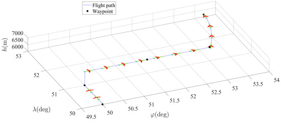
Figure 17. Flight path of the morphing aircraft with the morphing strategy proposed in Section 5.2.

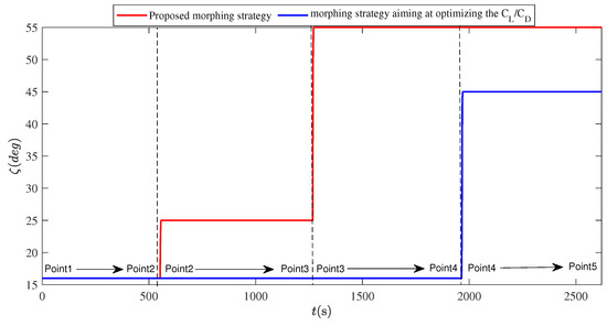
Figure 18. $\zeta$ of the comparative simulation in Section 5.2.

As seen in Figure 19 and Figure 20, between the waypoints 2 and 5, the fuel consumption of the proposed method is lower than that of the strategy aiming at optimizing lift-to-drag ratio. By comparing these two methods, the proposed method saves 2.48% in fuel consumption throughout the cruise mission. The reasons lie in two aspects: one is that the proposed strategy fully considers the variation in cruise conditions and equilibrium equations of forces, and it directly takes the engine thrust as the optimization target; thus, it can achieve more accurate morphing optimization to save fuel consumption; the other one is that the optimization of the lift-to-drag ratio under the current angle of attack is not rigorous enough, because the cruise angle of attack varies with the configurations, as can be seen in Figure 21, There is a significant difference between the cruise angles of attack between waypoints 3 and 5 for the configurations with $\zeta ={16}^{°}$ and $\zeta ={55}^{°}$. Therefore, although the $\zeta ={16}^{°}$ configuration has a larger lift-to-drag ratio, it still needs more thrust to overcome the drag at a larger cruise angle of attack.

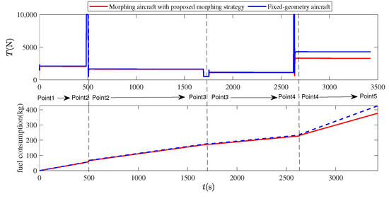
Figure 19. Engine thrust and fuel consumption of the comparative simulation in Section 5.2.

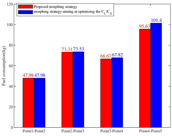
Figure 20. Fuel consumption for each cruise phase of the comparative simulation in Section 5.2.

Figure 21. Cruise angle of attack of the comparative simulation in Section 5.2.

5.3. Comparison with Morphing Decision Process without the Anti-disturbance Mechanism

In this subsection, the effectiveness of the proposed anti-disturbance mechanism is demonstrated; thus, we compare the proposed morphing strategy with the strategy that removes the anti-disturbance mechanism, i.e., directly making ${\zeta }_{des}={\zeta }^{\ast }$. Set the cruise mission as shown in Table 6 and the initial states of the morphing aircraft and the integrators as shown in Table 7. Consider a scenario wherein the morphing aircraft suffers from a fluctuating headwind $V_w$ and an airspeed measurement error d, where the magnitude of $V_w$ satisfies a Gaussian distribution with a mean of 10 and variance of 4, and d also satisfies a Gaussian distribution with a mean of 0 and variance of 2.

Table 6. Waypoint settings in Section 5.3.

Number	$\mathit{\phi }$	$\mathit{\lambda }$	h	${\mathit{V}}_{\mathit{e}}$
Point1	${40}^{°}$	${40}^{°}$	4000 m
Point2	$40.5^{°}$	${40}^{°}$	4000 m	270 m/s
Point3	$41.5^{°}$	${40}^{°}$	6000 m	220 m/s

Table 7. Initial state settings of the morphing aircraft and the integrators in Section 5.3.

Name	Value	Name	Value	Name	Value
${\phi }_0$	${40}^{°}$	${\lambda }_0$	${40}^{°}$	$h_0$	4000 m
$V_0$	270 m/s	${\chi }_0$	$0^{°}$	${\gamma }_0$	$0^{°}$
${\mu }_0$	$0^{°}$	${\alpha }_0$	$0.{73}^{°}$	${\beta }_0$	$0^{°}$
$p_0$	$0^{°}$/s	$q_0$	$0^{°}$/s	$r_0$	$0^{°}$/s
$I_{ev0}$	10	$I_{e\chi 0}$	0	$I_{e\gamma 0}$	0
$I_{e\mu 0}$	0	$I_{e\alpha 0}$	0	$I_{e\beta 0}$	0
$I_{ep0}$	0	$I_{eq0}$	0	$I_{er0}$	0
$T_0$	1430 N	$m_0$	$1250\mathrm{kg}$

As seen in Figure 22 and Figure 23, the proposed method selects a configuration with $\zeta ={55}^{°}$ between waypoints 1 and 2 and $\zeta ={16}^{°}$ between waypoints 2 and 3; the morphing strategy that does not include an anti-disturbance mechanism induces the chattering of $\zeta$ between waypoints 2 and 3. This is because the fluctuating airspeed measurements lead to high-frequency switching of ${\zeta }^{\ast }$.

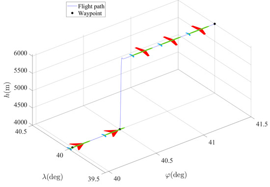
Figure 22. Flight path of the morphing aircraft with the proposed morphing strategy in Section 5.3.

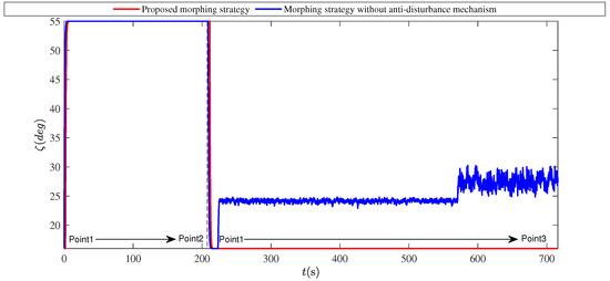
Figure 23. $\zeta$ of the comparative simulation in Section 5.3.

As seen in Figure 24, the chattering of $\zeta$ causes high-frequency oscillations in $\alpha$, q, and ${\delta }_e$, which are not allowed in engineering practice. Based on the above analysis, we can conclude that it is effective and necessary to introduce an anti-disturbance mechanism in the morphing decision process.

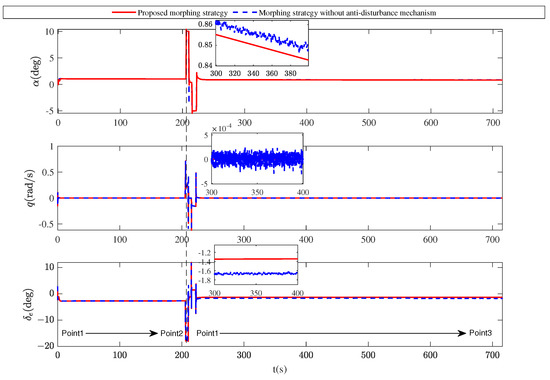
Figure 24. $\alpha$, q, and ${\delta }_e$ of the comparative simulation in Section 5.3.

6. Conclusions

We have considered the morphing decision problem for morphing aircraft with the objective of optimizing cruise efficiency. The following conclusions can be drawn:

• We propose a morphing decision strategy to optimize the cruising efficiency for a variable-sweep morphing aircraft, which consists of a nonlinear programming-based offline database and a database-based online morphing decision process. This strategy takes into account the variations in cruise airspeed, altitude, total mass, and the cruise angles of attack; thus, it can give the morphing decisions reasonably and accurately.
• In engineering practice, the effects of wind velocity and sensor errors lead to fluctuating airspeed measurements, which may cause high-frequency switching of the optimal configuration. To solve this problem, we introduce an anti-disturbance mechanism in the morphing decision process, which ensures that the optimized morphing decision can be given correctly and the high-frequency switching does not occur under fluctuating airspeed measurement conditions.
• The effectiveness of the proposed strategy has been validated by simulation. The results demonstrate that even after taking into account the additional of 75 kg caused by the morphing mechanism, the morphing aircraft with the proposed morphing strategy still has higher cruise efficiency than the fixed-geometry aircraft, especially in high-speed cruise conditions, where 22.4% of fuel consumption is saved. Further, the results show that the fuel consumption by the proposed strategy is 2.48% lower than that of the morphing strategy that aims at optimizing the lift-to-drag ratio. Furthermore, the proposed method demonstrably has a certain anti-disturbance ability for fluctuating airspeed measurements.

In the future, we will focus on designing a high-performance, online morphing decision strategy with a small computational burden and a strong anti-disturbance capability, and it does not require the support of an offline database. Another potential direction for the future work is the cruising efficiency optimization for the morphing aircraft model with more degrees of freedom for shape change.

References

- Li, D.C.; Zhao, S.W.; Da Ronch, A.; Xiang, J.W.; Drofelnik, J.; Li, Y.C.; Zhang, L.; Wu, Y.N.; Kintscher, M.; Monner, H.P.; et al. A review of modelling and analysis of morphing wings. Prog. Aerosp. Sci. 2018, 100, 46–62. [Google Scholar] [CrossRef]
- Barbarino, S.; Bilgen, O.; Ajaj, R.M.; Friswell, M.I.; Inman, D.J. A Review of Morphing Aircraft. J. Intell. Mater. Syst. Struct. 2011, 22, 823–877. [Google Scholar] [CrossRef]
- Guo, T.; Feng, L.; Zhu, C.; Zhou, X.; Chen, H. Conceptual Research on a Mono-Biplane Aerodynamics-Driven Morphing Aircraft. Aerospace 2022, 9, 380. [Google Scholar] [CrossRef]
- Mills, J.; Ajaj, R. Flight Dynamics and Control Using Folding Wingtips: An Experimental Study. Aerospace 2017, 4, 19. [Google Scholar] [CrossRef]
- Chen, M.H.; Liu, J.C.; Skelton, R.E. Design and control of tensegrity morphing airfoils. Mech. Res. Commun. 2020, 103, 103480. [Google Scholar] [CrossRef]
- Sahin, H.; Kose, O.; Oktay, T. Simultaneous autonomous system and powerplant design for morphing quadrotors. Aircr. Eng. Aerosp. Technol. 2022, 94, 1228–1241. [Google Scholar] [CrossRef]
- Yan, B.; Li, Y.; Dai, P.; Xing, M. Adaptive Wing Morphing Strategy and Flight Control Method of a Morphing Aircraft Based on Reinforcement Learning. J. Northwestern Polytech. Univ. 2019, 37, 656–663. [Google Scholar] [CrossRef]
- Yan, B.B.; Li, Y.; Dai, P.; Liu, S.X. Aerodynamic Analysis, Dynamic Modeling, and Control of a Morphing Aircraft. J. Aerosp. Eng. 2019, 32, 04019058. [Google Scholar] [CrossRef]
- Xu, W.; Li, Y.; Lv, M.; Pei, B. Modeling and switching adaptive control for nonlinear morphing aircraft considering actuator dynamics. Aerosp. Sci. Technol. 2022, 122, 107349. [Google Scholar] [CrossRef]
- Wang, Q.; Gong, L.; Dong, C.Y.; Zhong, K.W. Morphing aircraft control based on switched nonlinear systems and adaptive dynamic programming. Aerosp. Sci. Technol. 2019, 93, 105325. [Google Scholar] [CrossRef]
- Cheng, H.Y.; Dong, C.Y.; Jiang, W.L.; Wang, Q.; Hou, Y.Z. Non-fragile switched H-infinity control for morphing aircraft with asynchronous switching. Chin. J. Aeronaut. 2017, 30, 1127–1139. [Google Scholar] [CrossRef]
- Gao, L.; Zhu, Y.; Liu, Y.; Zhang, J.; Liu, B.; Zhao, J. Analysis and Control for the Mode Transition of Tandem-Wing Aircraft with Variable Sweep. Aerospace 2022, 9, 463. [Google Scholar] [CrossRef]
- Yue, T.; Zhang, X.Y.; Wang, L.X.; Ai, J.Q. Flight dynamic modeling and control for a telescopic wing morphing aircraft via asymmetric wing morphing. Aerosp. Sci. Technol. 2017, 70, 328–338. [Google Scholar] [CrossRef]
- Guo, J.; Wu, L.; Zhou, J. Compound Control System Design for Asymmetric Morphing-Wing Aircraft. J. Astronaut. 2018, 39, 52–59. [Google Scholar] [CrossRef]
- Dong, C.Y.; Lu, Y.; Wang, Q. Tracking Control Based on Control Allocation with an Innovative Control Effector Aircraft Application. Math. Probl. Eng. 2016, 2016, 5037678. [Google Scholar] [CrossRef]
- Liu, C.S.; Zhang, S.J. Novel robust control framework for morphing aircraft. J. Syst. Eng. Electron. 2013, 24, 281–287. [Google Scholar] [CrossRef]
- Gong, C.; Chi, F.; Gu, L.; Fang, H. Optimal control method for distributed morphing aircraft based onKarhunen-Loeve expansion. Acta Aeronaut. Astronaut. Sin. 2018, 39, 121518. [Google Scholar]
- Wang, J.; Chen, X.; Hong, H.; Li, C.; Gong, C.; Fu, J. Trajectory optimization of morphing aircraft based on multi-fidelity model. J. Northwestern Polytech. Univ. 2022, 40, 618–627. [Google Scholar] [CrossRef]
- Chen, X.Y.; Li, C.N.; Gong, C.L.; Gu, L.X.; Da Ronch, A. A study of morphing aircraft on morphing rules along trajectory. Chin. J. Aeronaut. 2021, 34, 232–243. [Google Scholar] [CrossRef]
- Wen, N.; Liu, Z.; Zhu, L.; Sun, Y. Deep Reinforcement Learning and Its Application on Autonomous Shape Optimization for Morphing Aircrafts. J. Astronaut. 2017, 38, 1153–1159. [Google Scholar] [CrossRef]
- Sang, C.; Guo, J.; Tang, S.; Wang, X.; Wang, Z. Autonomous deformation decision making of morphing aircraft based on DDPG algorithm. J. Beijing Univ. Aeronaut. Astronaut. 2022, 48, 910–919. [Google Scholar] [CrossRef]
- Li, R.Z.; Wang, Q.; Liu, Y.A.; Dong, C.Y. Morphing Strategy Design for UAV based on Prioritized Sweeping Reinforcement Learning. In Proceedings of the 46th Annual Conference of the IEEE-Industrial-Electronics-Society (IECON), Singapore, 18–21 October 2020; pp. 2786–2791. [Google Scholar] [CrossRef]
- Kose, O.; Oktay, T. Simultaneous quadrotor autopilot system and collective morphing system design. Aircr. Eng. Aerosp. Technol. 2020, 92, 1093–1100. [Google Scholar] [CrossRef]
- Seigler, T. Dynamics and Control of Morphing Aircraft. Ph.D. Thesis, Virginia Tech., Blacksburg, VA, USA, 2005. [Google Scholar]
- Love, M.; Zink, S.; Stroud, R.; Bye, D.; Chase, C. Impact of Actuation Concepts on Morphing Aircraft Structures. In Proceedings of the AIAA/ASME/ASCE/AHS/ASC Structures, Structural Dynamics and Materials Conference, Palm Springs, CA, USA, 19–22 April 2004. [Google Scholar] [CrossRef]
- Sooy, T.J.; Schmidt, R.Z. Aerodynamic predictions, comparisons, and validations using missile DATCOM (97) and aeroprediction 98 (AP98). J. Spacecr. Rocket. 2005, 42, 257–265. [Google Scholar] [CrossRef]
- Fiorentini, L.; Serrani, A. Adaptive restricted trajectory tracking for a non-minimum phase hypersonic vehicle model. Automatica 2012, 48, 1248–1261. [Google Scholar] [CrossRef]
- Lu, P.; van Kampen, E.J.; de Visser, C.; Chu, Q.P. Aircraft fault-tolerant trajectory control using Incremental Nonlinear Dynamic Inversion. Control Eng. Pract. 2016, 57, 126–141. [Google Scholar] [CrossRef]
- Stevens, B.L.; Lewis, F.L. Aircraft Control and Simulation: Vol. 76, Aircraft Engineering and Aerospace Technology; Wiley: New York, NY, USA, 2003. [Google Scholar]
- Snell, S.A. Nonlinear Dynamic-Inversion Flight Control of Supermaneuverable Aircraft. Ph.D. Thesis, University of Minnesota, Minneapolis, MN, USA, 1991. [Google Scholar]
- Sieberling, S.; Chu, Q.P.; Mulder, J.A. Robust Flight Control Using Incremental Nonlinear Dynamic Inversion and Angular Acceleration Prediction. J. Guid. Control Dyn. 2010, 33, 1732–1742. [Google Scholar] [CrossRef]
- Gill, P.E. User’s Guide for NPSOL Version 4.0; Report; Department of Operations Research, Stanford University: Stanford, CA, USA, 1986. [Google Scholar]
- Holmstrom, K.; Goran, A.O.; Edvall, M.M. User’s Guide for TOMLAB 4.5; Report; Tomlab Optimization Inc.: Seattle, WA, USA, 2004. [Google Scholar]
Disclaimer/Publisher’s Note: The statements, opinions and data contained in all publications are solely those of the individual author(s) and contributor(s) and not of MDPI and/or the editor(s). MDPI and/or the editor(s) disclaim responsibility for any injury to people or property resulting from any ideas, methods, instructions or products referred to in the content. |
© 2023 by the authors. Licensee MDPI, Basel, Switzerland. This article is an open access article distributed under the terms and conditions of the Creative Commons Attribution (CC BY) license (https://creativecommons.org/licenses/by/4.0/).