Review

Decadal Patterns of Westerly Winds, Temperatures, Ocean Gyre Circulations and Fish Abundance: A Review

1
Graduate School of Oceanography (GSO), University of Rhode Island (URI), Narragansett, RI 02882, USA
2
Your Ocean Consulting, LLC, 9924 Rainbow Dr., Knoxville, TN 37921, USA
3
RPS ASA, 55 Village Square Drive, South Kingston, RI 02879, USA
4
National Oceanic and Atmospheric Administration, National Marine Fisheries Service, Northeast Fisheries Science Center, Narragansett Laboratory, 28 Tarzwell Drive, Narragansett, RI 02882, USA
*
Author to whom correspondence should be addressed.
Climate 2015, 3(4), 833-857; https://doi.org/10.3390/cli3040833
Submission received: 20 July 2015 / Revised: 10 September 2015 / Accepted: 15 September 2015 / Published: 20 October 2015

Abstract

:
The purpose of this review is to describe the global scope of the multidecadal climate oscillations that go back at least, through several hundred years. Literature, historic data, satellite data and global circulation model output have been used to provide evidence for the zonal and meridional jet stream patterns. These patterns were predominantly zonal from the 1970s to 1990s and switched since the 1990s to a meridional wind phase, with weakening jet streams forming Rossby waves in the northern and southern hemispheres. A weakened northern jet stream has allowed northerly winds to flow down over the continents in the northern hemisphere during the winter period, causing some harsh winters and slowing anthropogenic climate warming regionally. Wind oscillations impact ocean gyre circulation affecting upwelling strength and pelagic fish abundance with synchronous behavior in sub Arctic gyres during phases of the oscillation and asynchronous behavior in subtropical gyres between the Atlantic and Pacific oceans.

Preface

This paper does not present rigorous statistics evaluating hypotheses and relies on qualitative descriptions and comparisons between relatively short time series. The hypotheses simplify the complexity of meteorological, oceanographic and fisheries processes seeking broad patterns. Observations of zonal and meridional wind patterns have been necessarily limited to 1.7 cycles since about 1900. This implies that the discussion of warm and cold or zonal and meridional patterns focuses on three or four data points. Proxies of past cycles can not be supported by the unobserved decadal variability in global winds. With roughly four data points, statistical power of any comparisons are very low, especially given the instances of mismatches by a decade or more are not considered important. Ultimately with continuation of global observing systems, with the use of coupled atmosphere-ocean general circulation models (which do not rely on observational data) such patterns may be revealed. In this review we strive to address questions which connect current findings on ocean basins’ climate interactions over a global scale: Do output from these models support global synchrony in atmospheric wind patterns, oceanic gyre circulations, and vertical velocities in the ocean? Does the ecology of fish populations reveal underlying global wind process? We hope the following discussion provides a holistic view that ties together multidisciplinary information in a succinct fashion that is constructive and thought provoking for future work.

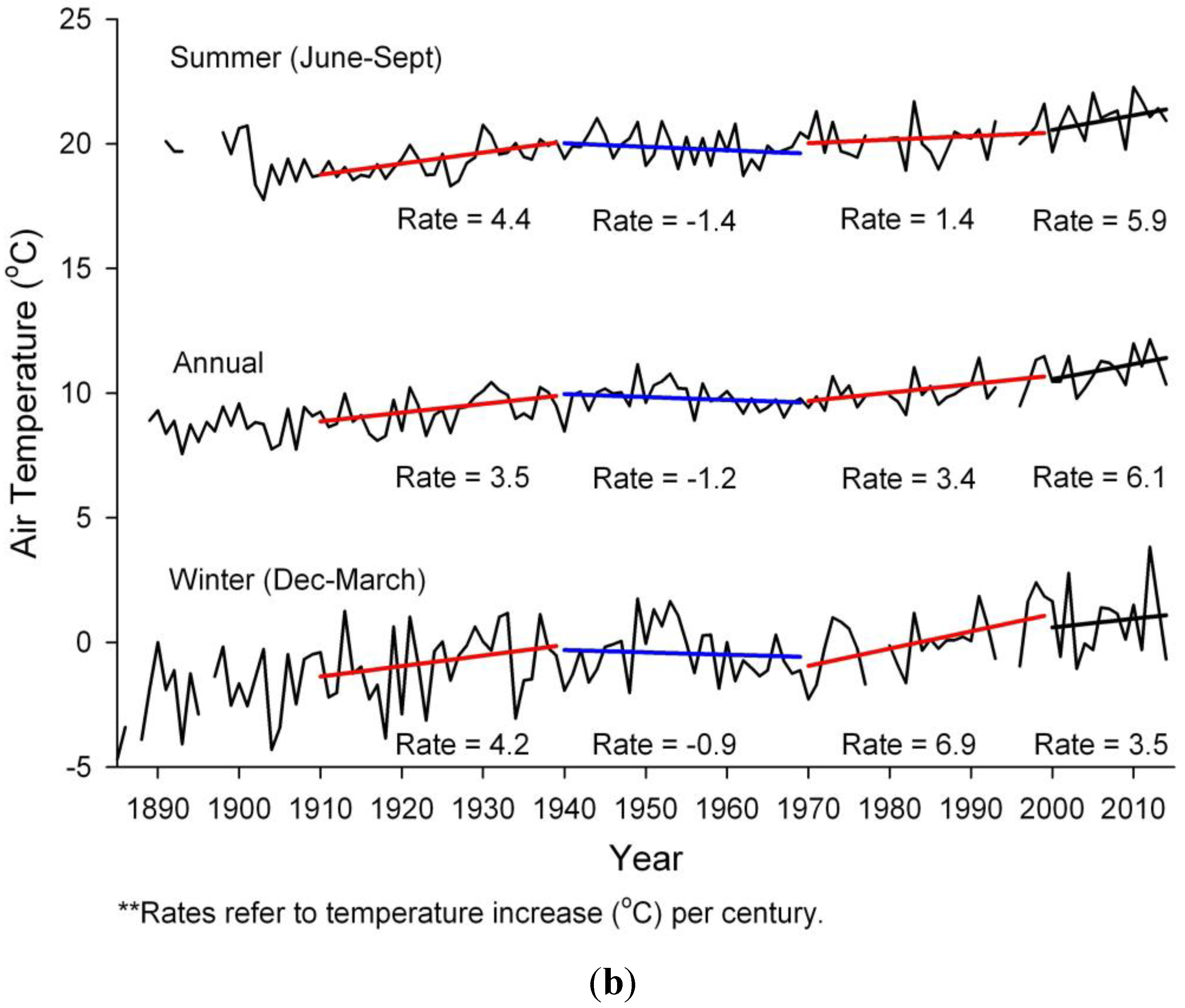
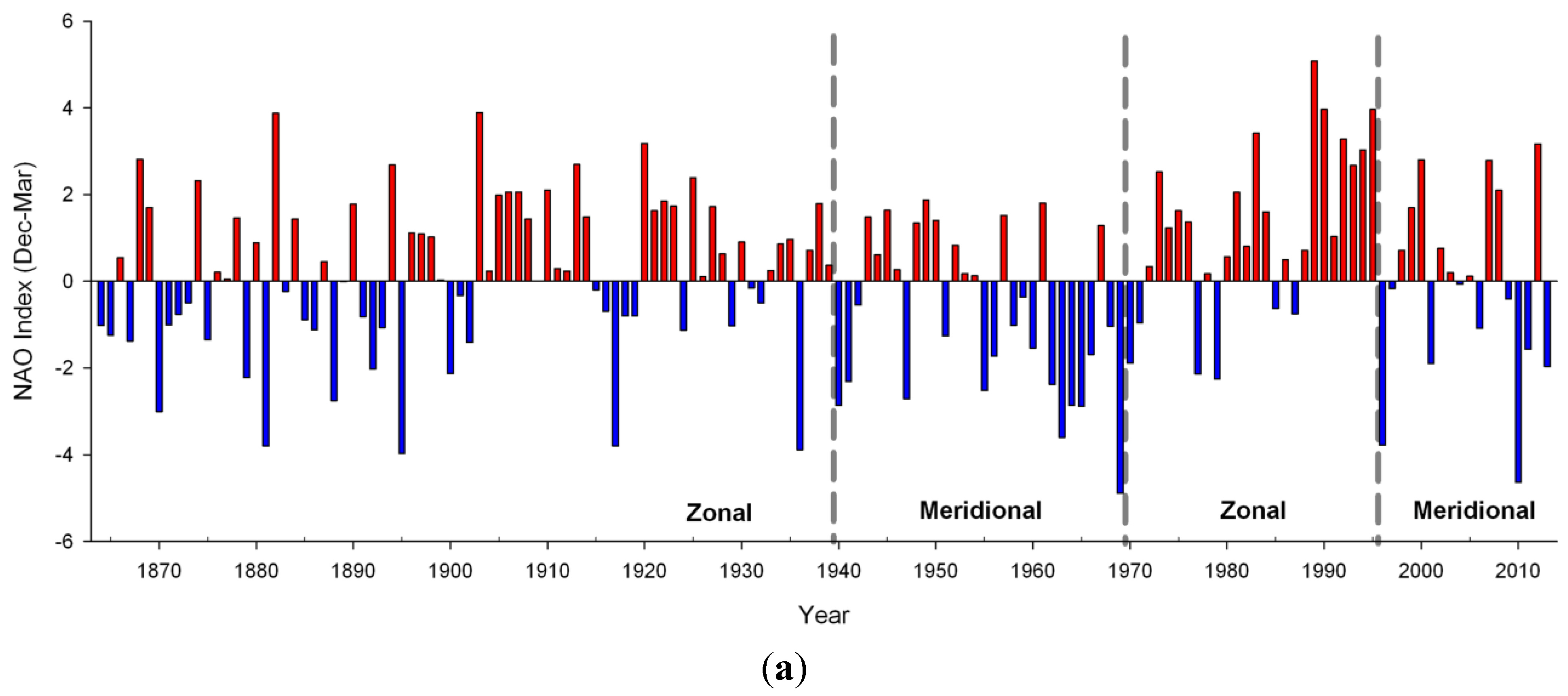
1. The Decadal Oscillation

During the 1990s, the global climate began to switch to a meridional wind or regionally cool cycle. Evidence of this switch was observed across climate indices, such as the North Atlantic Oscillation (NAO, Figure 1), the Arctic Oscillation (AO), the pattern of sea level pressure variation north of 20°N, and the Northern and Southern Annular Modes (NAM and SAM). Each of these indices represent different measures of jet stream behavior in the North Atlantic, northern hemisphere and the southern hemisphere, respectively. The NAO is defined by sea level pressure differences between the low pressure cell around Iceland and the high pressure cell around the Azores [1]. A positive NAO index indicates a large pressure difference between Iceland and the Azores, whereas a negative index indicates a small pressure difference [1]. The NAO is essentially a measure of the variability of the zonal flow with strong zonal flow during the positive cycle and meridional Rossby wave blocking north-south patterns during the negative cycle [2]. Mann and Lazier [3] have taken the work of Klyashtorin [4], Beamish et al. [5] and other earlier researchers to recognize the relationship between the above indices and many other climate indices including the Southern Ocean Index, the Pacific Decadal Oscillation, the Aleutian Low Pressure Index, the Atmospheric Circulation Index, the Pacific Circulation Index, and the Length of Day Index to reveal the similarity in patterns over the 20th century and correlations with fish abundances. All of these indices indicate zonal wind patterns in the early 20th century were succeeded by meridional patterns in the mid century and zonal patterns in the latter 20th century [3] (Figure 1). Several workers report decadal climate variability for particular ocean areas with similar phases to those presented in Figure 1. Similar phases are exhibited in the North Pacific Index (NPI) or the Pacific Decadal Oscillation (PDO) index [6] and correspond to shifts in salmon production in the North Pacific Ocean [7]. During the positive 20th century NAO periods, temperatures tend to increase, particularly in winter while during the negative period 1940 to1970 temperatures decrease (Figure 1b). During the late 1990s an apparent hiatus in decadal-scale warming occurred at mid-latitudes of the Northern Hemisphere. This observed stall in average surface-temperature increase was consistent with the mid-20th century behavior associated with a reversal of large-scale wind patterns, from zonal winds to meridional winds. The multidecadal component of climate variability is distinct from the secular-scale one, which is presumed to be of anthropogenic origin and apparently gaining strength in the 20th century (Figure 1). Interaction between these two components of climate variability remains an active topic of research. An important hypothesis in this review is that the changes in atmospheric circulation indicated by these indices result in changes in ocean gyre circulation over multidecadal time scales.

2. Objective: To Reveal The Connections Between The Decadal Oscillation of Atmospheric Wind Patterns and Ocean GRYRE Circulation

In this review a large literature supports the hypothesized components of interacting global wind pattern and ocean gyre circulation and reveals the decadal oscillation operates at a global system level. These decadal climate variations are not just characteristic of recent decades and the indices for these variations can be extended back through the centuries using proxy temperature records (Figure 2). Naturally occurring atmospheric jet stream and oceanic circulation cycles have occurred over at least the past 1500 years as evidenced in temperature proxy measurements that indicate warm to cool temperature cycles that occur on multidecadal time scales, such as tree rings, ocean sediment cores and coral bands [8,9]. The increasing error of proxy records in more distant centuries are acknowledged in uncertainty analyses for all data [8] and are shown here as best estimates (Figure 2). Decadal changes in the strength of jet stream westerly winds in both hemispheres alter ocean gyre circulations and together with trade winds, the upwelling intensity off continental margins.
Figure 1. (a) Winter (December, January, February and March) NAO indices from 1864–2013. The indices highlight the cool/warm phase shifts over the past century. Winter NAO indices were obtained from the Climate and Global Dynamics Division of the National Center for Atmospheric Research [10]. (b) Annual, summer and winter average air temperatures observed at Providence, Rhode Island (41.7°N, 71.4°W) from 1900–2014. Overlaid on these data are trend lines of temperature during each of the NAO oscillation cycles (positive: 1910–1940; negative: 1940–1970; positive: 1970–1995); negative 2000–2014 with a red line indicating a positive oscillation phase, and a blue line indicating a negative oscillation phase. Data were accessed through the Goddard Institute for Space Studies, National Aeronautics and Space Administration [11]. General adjusted surface temp data is provided to GISS monthly by NOAA/NCEI in the form of GHCNv3 data with SCAR temps to account for Antarctic regions. While changes have been made in the adjustment algorithms since 2011/2012 (it used to be GHCNv2), the changes have been to increase accuracy and therefore GHCNv3 data are most accurate. Temperatures continue to increase, with winter rates increasing markedly during the two warm periods. During the current incomplete negative oscillation period 2000–2014 temperature increases are still all positive but less so during the winter; the regression line is colored black to acknowledge that cooling is not evident. The positive/negative trends with lower magnitude are revealed for the all proxy annual temperature for the northern hemisphere [8]: 1910–1940, 1940–1970, 1970–2000 with 1.87, −0.48, 1.83 °C per 100 years, respectively.
Climate 03 00833 g001aClimate 03 00833 g001b
Support for the hypothesized wind/ocean gyre circulation interaction resides in the relationship whereby global decadal westerly wind and gyre circulations have a mirrored impact in upwelling ecology. As suggested by many researchers the variation in upwelling intensity can change the dominance of fish species populations. The dominant fish caught oscillate on decadal time scales between strong and weak upwelling preferring species. Klyashtorin [4] proposed a global connection between the hemispheric strength of the zonal versus meridional westerly winds and global landings of different fish stocks, although alterations in fish stocks have been observed for decades [12]. The biological responses to natural climate variability may be even more sensitive and predictable than the physical indicators [7].
Figure 2. (a) Mann Temperature anomalies (where the mean temperature is set to zero and differences from the mean are plotted) from all-proxy record for the Northern Hemisphere from 500 to 2006 indicate an increase in temperature from the 1800s on, adapted from the Mann et al. [8]. Trends in the record like the Little Ice Age and Global Warming have been removed by providing only the differences in adjacent maximum and minimum ranges (peaks and valleys) of temperatures and not the actual temperature. The difference between successive maximum and minimum were plotted from the zero line. The average cycle peak to peak from 500–2006 is 75 years. (b) The Mann temperature anomalies (red) and the Atlantic Multidecadal Oscillation from ship and satellite measurements: AMO smoothed from Kaplan Sea Surface Temperature version 2 calculated at NOAA/ESRL/PSD1 accessed July 2014 [13].
Climate 03 00833 g002

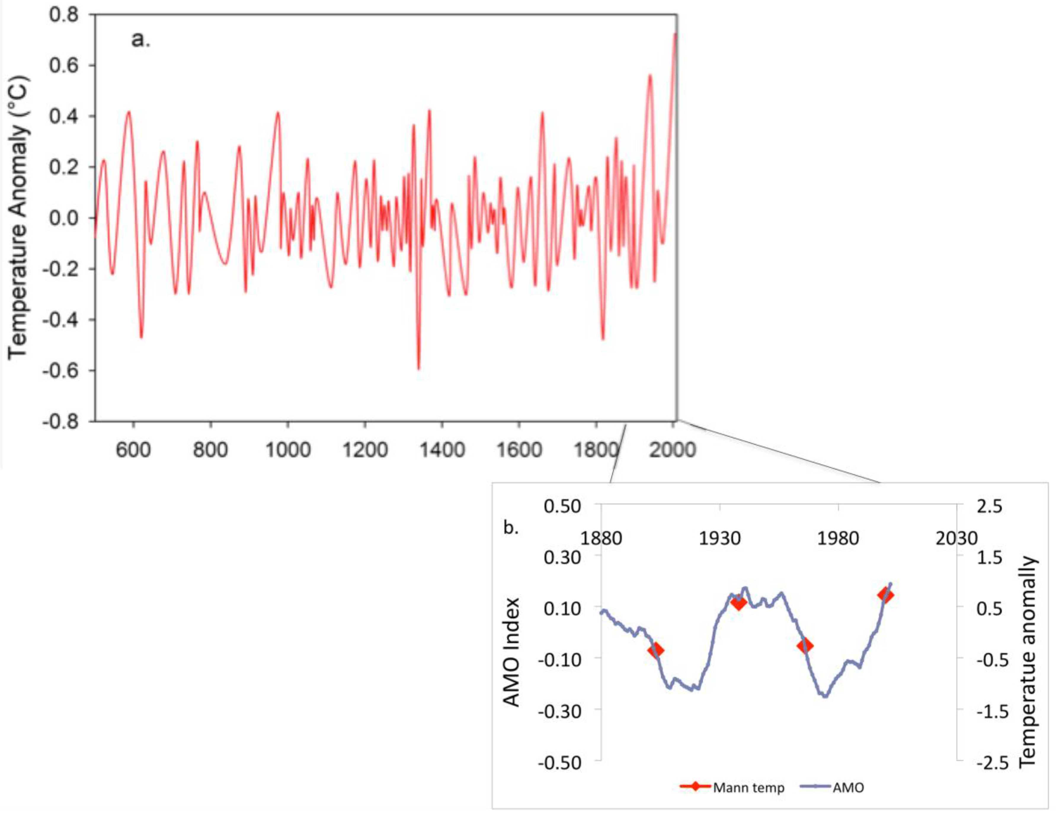
3. Causes for the Global Oscillation

Hypotheses to explain the decadal shifts are not mutually exclusive and include: (1) atmospheric-ocean interaction dynamics; (2) the rate of Atlantic meridional overturning circulation; and (3) a statistical combination of climate indices and Arctic sea ice variability. To date an accepted causation is uncertain for any of these proposals.
Figure 3. Global wind and gyre circulation changes hypothesized to be associated with multidecadal (a) warm and (b) cool phases of the North and South Hemispheres. White arrows indicate regions of enhanced wind and black arrows indicate areas of enhanced gyre circulation. The blue patches indicate the sinking waters in the North Atlantic. The zonal warm phase occurred from the 1910s to 1940s and 1970s to 1990s and is characteristic of strong westerly winds in the northern and southern hemisphere. North Pacific and North Atlantic subarctic gyre circulations enhance with sinking waters associated with the northern North Atlantic winter. In the Atlantic subtropical gyre circulations also enhance. Some surface waters travel from the Indian Ocean to the south Atlantic and join the Gulf Stream in the North Atlantic. The meridional cool phase occurring from the 1940s to 1970s and 1990s to present consists of equatorward winds over the continents and poleward winds over the subarctic and sub-antarctic oceans, resulting as Rossby wave formations. Intensified circulation in subtropical gyre systems enhances upwelling and productivity in the California and Peru systems. Strengthened easterly trade winds increase equatorial current circulation in the Pacific. The background global chlorophyll is from Yoder et al. [14].
Climate 03 00833 g003
Atmospheric scientists have maintained that winter NAO anomalies owe their existence to atmospheric processes [15]. They suggest that hemispheric winds of the NAM and SAM reflect dynamic processes that transcend land-sea geometry and the distribution and character of continents of a particular hemisphere. The NAO was thought to be a symptom of a broader fluctuation in the atmospheric mass between the entire Arctic Basin and the surrounding zonal ring [15]. In this way sea level pressure is described as a hemispheric scale seesaw of atmospheric mass between polar latitudes and the centers in the North Pacific and North Atlantic. The southern hemisphere has an identical low pressure polar area and high pressure zonal ring [15]. Generally the sea level pressure seesaw has a strong winter signature in the northern hemisphere [15] but is less seasonal in the southern hemisphere [16].
While NAO pressure centers represent mainly a winter index, the NAO signature is the dominant mode of the atmosphere throughout the year [17]. On a decadal scale a strong zonal jet stream has been associated with positive NAO anomalies and a weaker meridional jet stream with hemispheric Rossby waves has been associated with negative NAO anomalies (Figure 3). Thompson et al. [15] indicated that the polar vortex of westerly jet winds is hemispheric with zonal or meridional patterns simultaneously in northern and southern hemispheres (to observe similarity in northern hemisphere and southern hemisphere wind behavior patterns see: http://squall.sfsu.edu/crws/jetstream.html). During a cool/meridional phase, the westerly jet stream winds weaken forming moving wave patterns (Rossby waves). Three or four hemispheric waves form moving toward the equator over the continents and poleward over the oceans resulting in enhanced north-south, wind patterns in both hemispheres [3]. Some researchers have suggested that the recent switch to meridional winds, Rossby waves and severe winter weather was caused by Arctic ice melt and a reduced hemispheric temperature gradient [18]. This idea, however, has not been supported by other observational analyses or theory although it is still under review [19]. Weaker westerly winter winds cause the northern North Atlantic to become warmer as warm air is pushed northward over the ocean, and the Northern Hemisphere continents to become colder in winter as the Arctic winds are pushed south over the continents [1].
Evidence is slowly building to suggest that the North Atlantic ocean may have a significant impact on the atmosphere, specifically the stratosphere and multidecadal variation of the winter NAO. Scaife et al. [20] have revealed a strong correlation between stratospheric westerly winds and the NAO as well as between stratospheric and tropospheric westerly winds from 1965 to 1995. In the North Atlantic the Gulf Stream causes atmospheric variability in the form of wind divergence and convergence on the cold and warm boundaries, respectively, causing an upward motion across the Gulf Stream which extends into the upper troposphere [21]. The resulting upper tropospheric divergence may be important in generating stationary Rossby waves that produce remote responses. During winter months tropospheric wave forcing from ocean heat flux may enter the stratosphere, and with persistent anomalies on multidecadal time scales of 40 to 60 years, cause increased frequencies of sudden stratospheric warming according to coupled atmosphere-ocean global climate models [22]. An enhanced sudden stratospheric warming frequency may be connected to multidecadal negative NAO. Whether the NAO changes can be forced by ocean heat flux is controversial and global climate models of the stratosphere are apparently too limited in height to predict the interaction well. Supporting this connection, however, Omrani et al. [23] found that large scale Atlantic warming of the AMO apparently drove stratospheric warming resulting in a negative troposphere NAO in late winter since the mid 1990s. Thus their results suggest that the atmosphere does respond to ocean variability and that the potential exists for a self-maintaining oscillatory mode of internal ocean-atmospheric variability.
While this ocean-atmospheric feedback may explain westerly wind variability in the northern hemisphere, it does not explain the concurrent fluctuations of westerly winds in the southern hemisphere. Existing evidence does suggest some form of atmospheric communication from the northern hemisphere NAM to the southern hemisphere SAM. It is revealing that annular modes extend deep into the tropics and subtropics of the opposing hemisphere [24]. This signature is associated with respective winter seasons but stronger with the NAM. The NAM and the SAM have both exhibited high index polarity from 1979 to 1999 and particularly, the NAM contributed to climate trends in the tropics with a 0.1 K cooling of the tropical troposphere [24]. Building on this connection Fogt et al. [25] have found that SAM variability reconstruction displayed decadal peaks of at least 2 y duration, particularly in the austral spring and summer, in the1930s and 1960s which are not captured in global climate model comparisons. In SAM indices based on instrumental data and reanalysis data, Yuan and Yonekura [26] find another positive anomaly in the late 1990s with the amplitude of the this anomaly and the one in the 1960s, equivalent to the total change of the long-term trend from the 1950s to 1990s. A possible mechanism for these peaks could be strong NAM forcing of regime shifts through remote influences from the tropical troposphere-stratosphere.
A complication, is that wind indices, whether zonal or meridional, have temporally and spatially varied positions due to complicated dynamics and asymmetry of continents and mountain ranges in the northern hemisphere. Thus, measures of wind velocity, and particularly direction, like the annual Atmospheric Circulation Index (ACI) and the winter Pacific Circulation Index (PCI) have the same pattern with a time lag in the peak position of the PCI [2]. These indices are anomaly trends of winter wind-flow regimes and not real-time indices. The ACI originated from Russian workers Vangenheim [27,28] based on the long-term temperature and ice break-up forecasting over the North Atlantic, Europe and Asia, and Girs [5,29] based on number of days with wind patterns classified to three types, zonal, meridional, easterly (like meridional but opposite in phase) and adapted by Kylashtorin [4]. The PCI is derived from the same technique as the ACI but includes the atmosphere over the North Pacific and western North America for the winter period [3]. Climate indices not based on wind measures may fail to be statistically correlated between ocean basins [30].
Just as some hypotheses are related mainly to the atmosphere, others involve ocean circulation. Several authors interpret decadal variability as coupled atmosphere/ocean interactions over the North Atlantic [31]. One proposal is based on the rate at which surface North Atlantic waters sink during winter to form North Atlantic deep water, or the Atlantic Meridional Overturning Circulation (AMOC). Over decadal time scales, the latitudinal temperature gradient of the North Atlantic intensifies or decreases, presumably depending on the rate of the winter water sinking. These temperature changes have been recorded by ship and satellite sensors and summarized as the Atlantic Multidecadal Oscillation [32,33,34]. The AMO may be described as the time integrated effect of the NAO on ocean currents that results in an out of phase surface cool pool/warm pool in the North Atlantic during positive/negative NAO. The transition from warm pool to cool pool apparently occurs as the salty warm water, cools and sinks to thermocline depth mixing the heat into the deeper waters and cooling the surface waters of the North Atlantic, resulting in the recent regional stasis in global warming [35]. This mixing does not occur in other oceans except for the deeply mixed southern ocean [35]. In past cold glacial periods, ice prevented North Atlantic water from sinking; during glacial and early interglacial periods, ice sheets and/or great melt water lakes burst into the North Atlantic and prevented water from sinking, resulting in the return of glacial cold conditions [36]. These cold periods were followed by rapid North Atlantic water sinking and an increasingly warm climate [36]. Many researchers have suggested that the abrupt climate change in the glacial era associated with deep-water formation on/off is now in the current late interglacial era a decadal waxing and waning of deep-water formation as surface waters decrease in stratification/increase in stratification with fresh melt waters [37]. Knight et al. [32] has simulated the thermohaline circulation in the North Atlantic over the past 1400 years and predicts the waxing and waning of the surface circulation over the past centuries. While, deep Atlantic current measurements have so far not established a connection with North Atlantic deep-water formation and the NAO or AMO [38], the RAPID current array at 26.5°N over the period of 2004 to 2012 has indicated a decline of ~0.5 Sv·y−1 in the AMOC which exceeds the rate of decline due to climate warming of ~0.05 Sv·y−1 and may be due to decadal change [39].
A large literature discusses the movement of surface water and heat to the polar region of strongest deep-water formation, from the opposite pole, which is termed “heat piracy” [40,41]. The strength of the “piracy” depends upon the degree of balance in the formation of deepwater at the respective poles. While most of this literature is paleoceanographic, “piracy” is an active area of research in the modern ocean [42,43]. Broecker et al. [44] using chemical proxies have speculated about the north-south hemisphere seesaw slow down of Antarctic Bottom Water (AABW) formation in the Southern Hemisphere during the 20th century period compared to the meridional period of the Little Ice Age. According to their recent World Ocean Circulation Experiment and earlier current measurements, Ganachaud and Wunsch [45] find no such slow down in AABW formation in the late 20th century. This controversy continues with a recent publication suggesting that like the decrease in AABW formation, apparently due to excessive melt-water, during the last interglacial, a slowdown in AABW has occurred recently, as evidenced by the absence of polynya formation in the Weddell Sea, in the late 20th century during the zonal period of rapid North Atlantic Deep Water formation [46].
A new hypothesis for the northern hemisphere natural climate warming/cooling, centers on the oscillation of sea ice extent in the Arctic [47]. The multivariate “stadium wave” analysis incorporates the collective interaction of all major climate indices including new indices of sea ice in the Arctic. Multiple dynamics related to climate signal communication include migration of the Inter Tropical Convergence Zone, basin scale wind patterns, western boundary current dynamics and Arctic sea ice processes. The main mechanism, apparently controlling the oscillation of sea ice, is the Atlantic Ocean’s constructive/destructive influence on the Arctic halocline which is responsible for the winter time ice cover. A strong halocline promotes sea ice formation by preventing warmer deep waters from mixing to the surface and vice versa. Processes, which regulate Arctic freshwater balance, act continually to reverse the “stadium wave”. A strong halocline and extensive ice cover introduce a warm regime and vice versa. During the current cool regime the authors expect ice to increase in the Greenland, Barents and Kara Seas and the Arctic Seas of Siberia including Laptev, East Siberian and Chukchi Seas [47]. Kravtsov et al. [28] have further developed the stadium wave analysis, countered the criticism that this work represents a statistical artifact and urged an improved agreement between observations and simulations by a state of the art climate model.

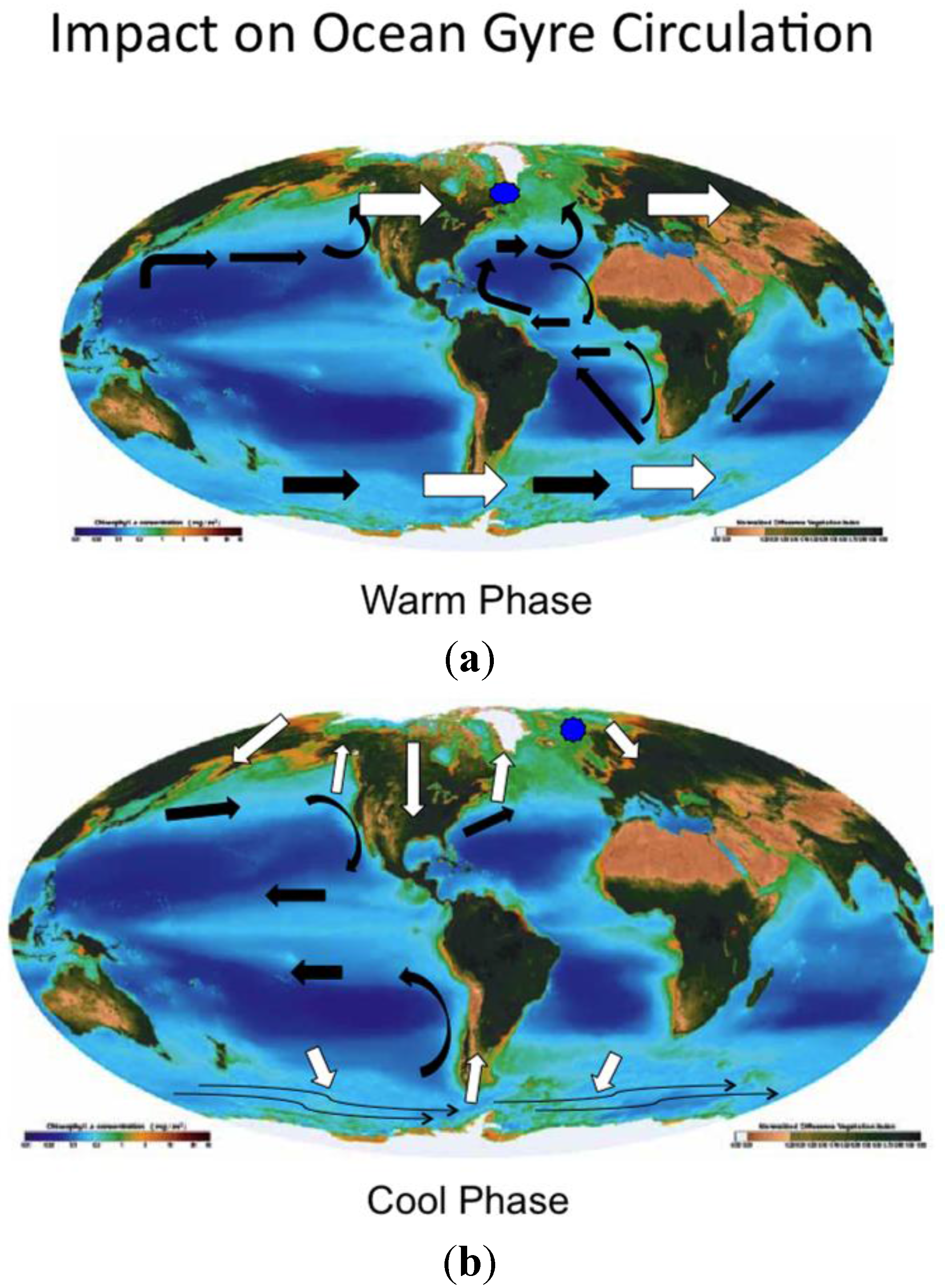
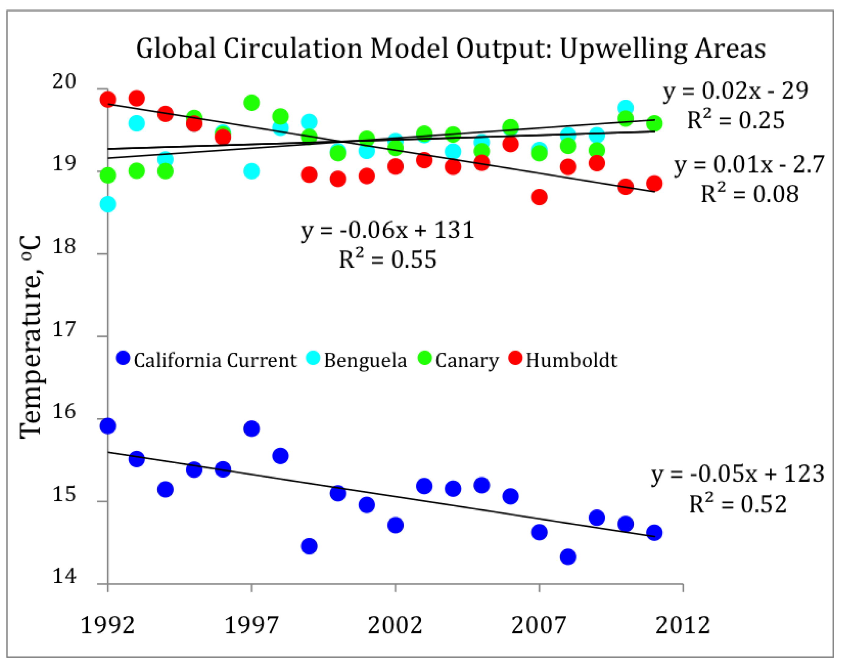
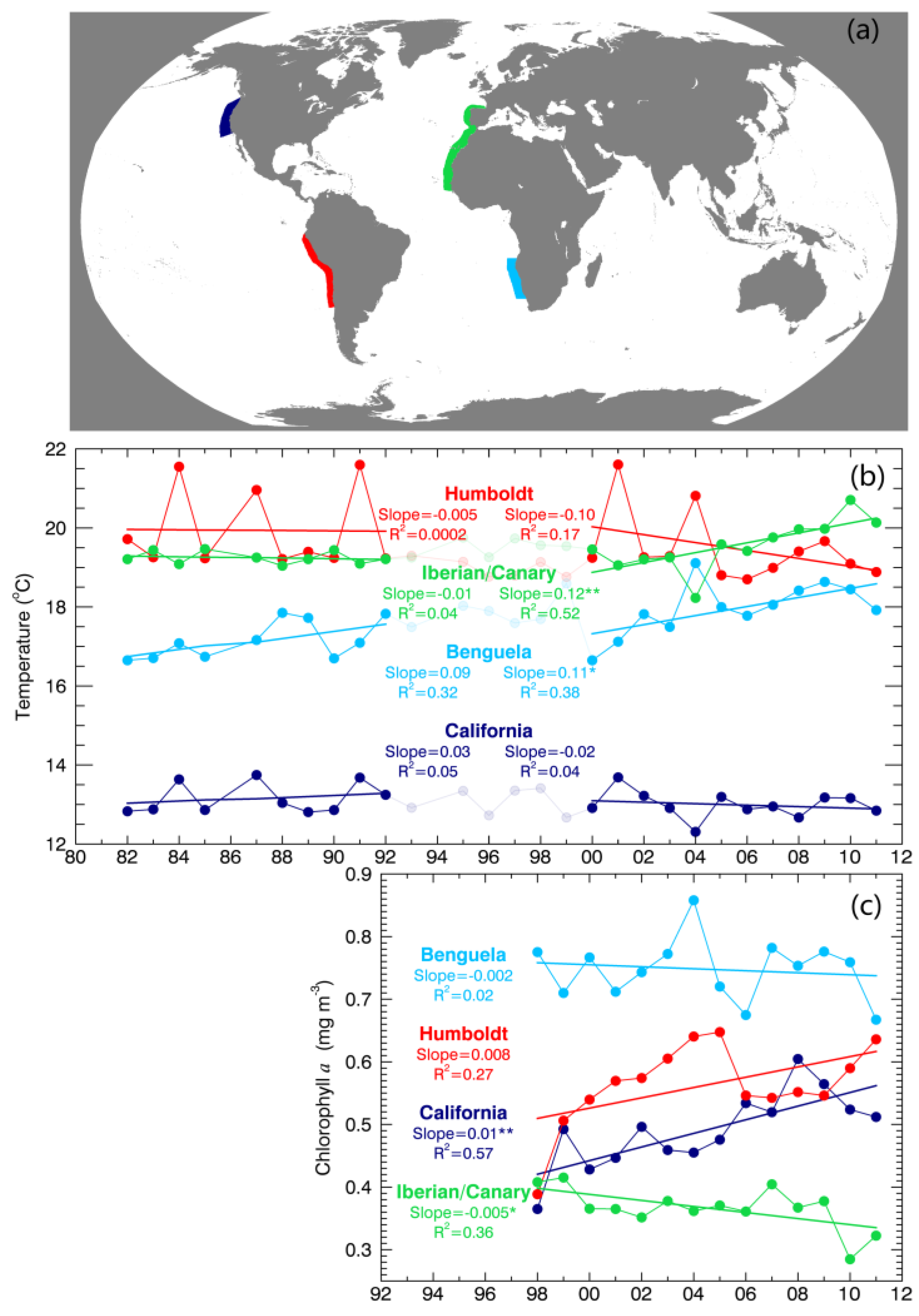
4. Oscillations in Gyre Circulation and Upwelling

For this review we have hypothesized changes in ocean gyre circulation and upwelling strength based on the literature, satellite data and a global ocean circulation model (Figure 3, Table 1). New ocean observation arrays will eventually provide data to document more fully changes in gyre circulations. During both decadal phases synchronous behavior occurs for the subarctic gyres but contrary to expectation, synchronous behavior apparently fails to occur for subtropical gyres. During the warm/zonal phase, the strength of the subarctic gyre circulation increases in the Atlantic and Pacific [48]. As subarctic gyres surge, subtropical gyres relax in the Pacific, but not in the Atlantic (Figure 3). In the North Atlantic, both subarctic and northern hemisphere subtropical gyre circulations increase [17]. Atlantic southern hemisphere subtropical gyre circulation may also increase but instrumental records are too short to test the hypothesis for a pan-Atlantic decadal oscillation [49]. The result would be out of phase circulations in subtropical gyres between the Pacific and Atlantic oceans. There is evidence during zonal phase of the Atlantic northeast tropical trade winds increasing, likely due to the location of the central east Atlantic high-pressure area [1,15]. In the tropical Atlantic, cross equatorial transport from the South Atlantic to the North Atlantic increased in the late 1970s to 89% compared to 32% in the late 1960s due to increased northern trade winds and Ekman transport (Figure 3) [42]. The out of phase circulation between subtropical gyres in the Atlantic and Pacific may be due to the thermohaline circulation of the Atlantic versus the lack of this circulation in the Pacific or to the smaller ocean mass relative to the greater land masses around the Atlantic compared to the Pacific or other unknown factors.
Table 1. Summary of upwelling wind speed trends over time (slope, mean, standard deviation (SD) and tendency), temperature tendency, chlorophyll tendency for early 2000s. n.d: no data.
Wind Speed-2 Degrees Latitude by 2 Degrees Longitude *
UpwellingSlopeMeanSDTendencyTemperature1Chlorophyll1
Location2 ms−1y−1ms−1ms−1°Cgm−3
Oyashio−0.0728.614.08slowingn.d.n.d.
California0.0268.063.97increasingcoolingincreasing
Humboldt0.0376.712.06increasingcoolingincreasing
Canary−0.0126.492.45slowingwarmingdecreasing
Benguela−0.0025.943.00slowingwarmingdecreasing
*Satellite microwave scatterometer 1999–2009, Jet Propulsion Laboratory data at http://oceanmotion.org/html/resources/wind.htm; 1 From Figure 4 and Figure 5; 2 Oyashio [158°E–160°E, 46°N–48°N], California [126°W–124°W, 38°N–40°N], Humboldt [80°W–78°W, 16°S–14°S], Canary [12°W–10°W, 32°N–34°N], Benguela [14°E–16°E, 30°S–28°S].
Observational atmospheric pressure and current data over the last 50 years in the North Atlantic indicate surging of both the North Atlantic subarctic and subtropical gyres during the warm/zonal, positive NAO phase [50]. The literature provides evidence of significant surface water winter sinking and movements of deep Atlantic water within the subarctic gyre, as well as between subarctic and subtropical gyres [50]. The North Atlantic current, the southward deep interior flows of the subarctic, and the southward deep interior flow of the subtropical gyre were also strong [50]. Further, the western far North Atlantic stayed cold, during this time period, as strong westerly winds isolated northern regions like the Labrador Sea, causing convective sinking in that region [51]. The westerly winds that isolate the cold to the north kept the more southerly North Atlantic and Western Europe warm. Annual average temperatures in the eastern and western Atlantic at temperate latitudes increased by 1 °C over the annual cycle and up to 2 °C during the winter period [52], (Figure 1). The overall subarctic Atlantic gyre circulation increased (~15%) with increasing westerlies in the latter twentieth century and subsequently relaxed in the mid 1990s to present [53,54]. The meridional regime has led to weaker Atlantic Ocean gyres notably since the 1990s [55].
Instrument records have been too short to reveal correlated multidecadal subtropical gyre circulation changes in the South Atlantic and North Atlantic (Figure 3) [49]. At shorter time scales South Atlantic subtropical gyre circulation has been observed to fluctuate at similar frequencies with the North Atlantic [56], and southern tropical Atlantic sea surface temperature have been correlated at decadal time scales [49]. There has been not-too-convincing evidence of mutidecadal changes in wind intensity in the south subtropical Atlantic. A St Helena Climate index, which apparently reflects the intensity of the southeasterly trades in the South Atlantic, shows strengthening from 1900 to the 1930s, weakening to stable conditions to the 1970s and then a weak strengthening from the 1980s to 2000 [57]. Despite the apparently weak St Helena Climate trends, upwelling intensity followed the expected patterns. The 1960 were characterized by weak upwelling favorable winds [58]; during the 1970s to 1990s, an increase in upwelling was observed along the Luderitz at ~26° off the west coast of Africa resulting in colder water temperatures, increased nutrients and chlorophyll concentrations close to the coast [57,58,59,60]. In the 1990s decreased wind stress, upwelling and increasing temperatures were observed along the northern Benguela current system [58,59,61]. It is perhaps, indicative that 3 Benguela Ninos occurred from 1960s to 1990 period and that 4 Benguela Ninos occurred during the 1990s [56] suggesting a weakening of the Southeast Trades in the latter decade compared to earlier decades. Good evidence does support the strengthening/weakening of the South Atlantic sub-polar gyre during strong/weak westerlies in the southern hemisphere on multidecadal time scales [62].
By contrast to the Atlantic, in the Pacific subtropical gyres, circulation and easterly trade winds have been observed to decrease during the warm/zonal phase of the oscillation [48,63] and El Nino becomes more frequent and intense in the tropical south Pacific [64]. A reconstruction of variability in the southeast Pacific from the late Holocene has shown that during strong zonal wind and Antarctic Circumpolar Current speed, strong upwelling of Antarctic Intermediate water develops and flows toward the equatorial Pacific [65]. The temperature contrast and mixing in equatorial thermocline waters modulates El Nino activity. After the late 1970s regime shift a high positive Southern Annular Mode dominated resulting in strong zonal winds [66]. Upwelling anomalies from the South Pacific perturbed the equatorial thermocline seven years later resulting in a series of strong El Nino events in the late 20th century [67]. As a result of the decreased equator-ward winds (northerly winds in the northern hemisphere and southerly winds in the southern hemisphere) and due to the weakened easterly trade winds in the tropics, upwelling off the western margins of continents decreases [17,63]. Prior to the mid 1970s the upwelling in the California current system was deeper; while during post mid 1970s the upwelling was shallower with more horizontal entrainment of surface waters from the north [68]. In the North Pacific the Pacific Decadal Oscillation (PDO—defined as the first empirical orthogonal function (EOF)/principal component (PC) of both sea surface temperature (SST) and sea surface height (SSH)) an atmospheric index of climate, gives different correlations with physical and biological parameters than the North Pacific Gyre Oscillation (NPGO—defined as the second EOF/PC of SST and SSH) Index representing an oceanic climate index [69]. The NPGO variability is statistically separate from the PDO and explains salinity and nutrient variability that the PDO does not and may be a better indicator of planktonic ecosystem dynamics. The NPGO may be a better index of upwelling along the southern California coast although the PDO appears to be better north of 38°N [69].
Figure 4. (a) Global map showing upwelling regions and (b) year versus annual sea surface temperature (based on satellite data) in upwelling regions (color coded) of the Benguela, Humboldt and California currents. An upward trend suggests slowing upwelling, no trend suggests steady upwelling and a downward trend suggests increased upwelling; and (c) SeaWiFS and MODIS annual surface chlorophyll concentration in upwelling areas in Benguela, Humboldt, California and Iberia/Canary. Oyashio data quality too questionable to present. For this figure Satellite derived (AVHRR Pathfinder [70]) and chlorophyll (SeaWiFS and MODIS [71]) data were compiled from upwelling regions (Table 2). Pathfinder data were provided by GHRSST and the US National Oceanographic Data Center (http://pathfinder.nodc.noaa.gov). This project was supported in part by a grant from the NOAA Climate Data Record (CDR) Program for satellites.
Climate 03 00833 g004
Figure 5. The Massachusetts Institute of Technology (MIT) global circulation model temperature for upwelling zones in Figure 4a. Slopes of linear regression lines indicate coherence with Figure 4b and are positive for Canary and Benguela and negative for California and Humboldt currents for available model output period 1992 to 2012. The state estimates were provided by Estimating the Circulation and Climate of the Ocean, Phase II (ECCO2) Consortium for Estimating the Circulation and Climate of the Ocean funded by the National Oceanographic Partnership program (NOPP).
Climate 03 00833 g005
As the westerly winds weaken and north-south winds and trade winds strengthen during the cold/meridional phase in both hemispheres of the Pacific, subtropical gyre circulations are observed to increase [48,63,72]. In the North Pacific the NPGO was observed to strengthen since 1993 [69]. Intensified circulation in subtropical gyre systems and intensified trade winds enhances upwelling and productivity in the California and Humboldt systems [73,74,75]. Gyre circulation in the South Pacific has intensified by 20% at 1000 m since the 1990s [76].
Table 2. Latitude and longitude location of corners of color code areas for Figure 4a.
SubareaUL_LONUL_LATUR_LONUR_LATLL_LONLL_LATLR_LONLR_LAT
California Current128.8047.94−119.2247.94−128.8032.39−119.2232.39
Humboldt Curent−82.66−4.35−70.00−4.35−82.66−33.09−70.00−33.09
Iberian Canary Current−20.5244.96−1.5444.96-20.5211.73−1.5411.73
Benguela Current8.04−14.1117.09-14.118.04−29.7517.09−29.75

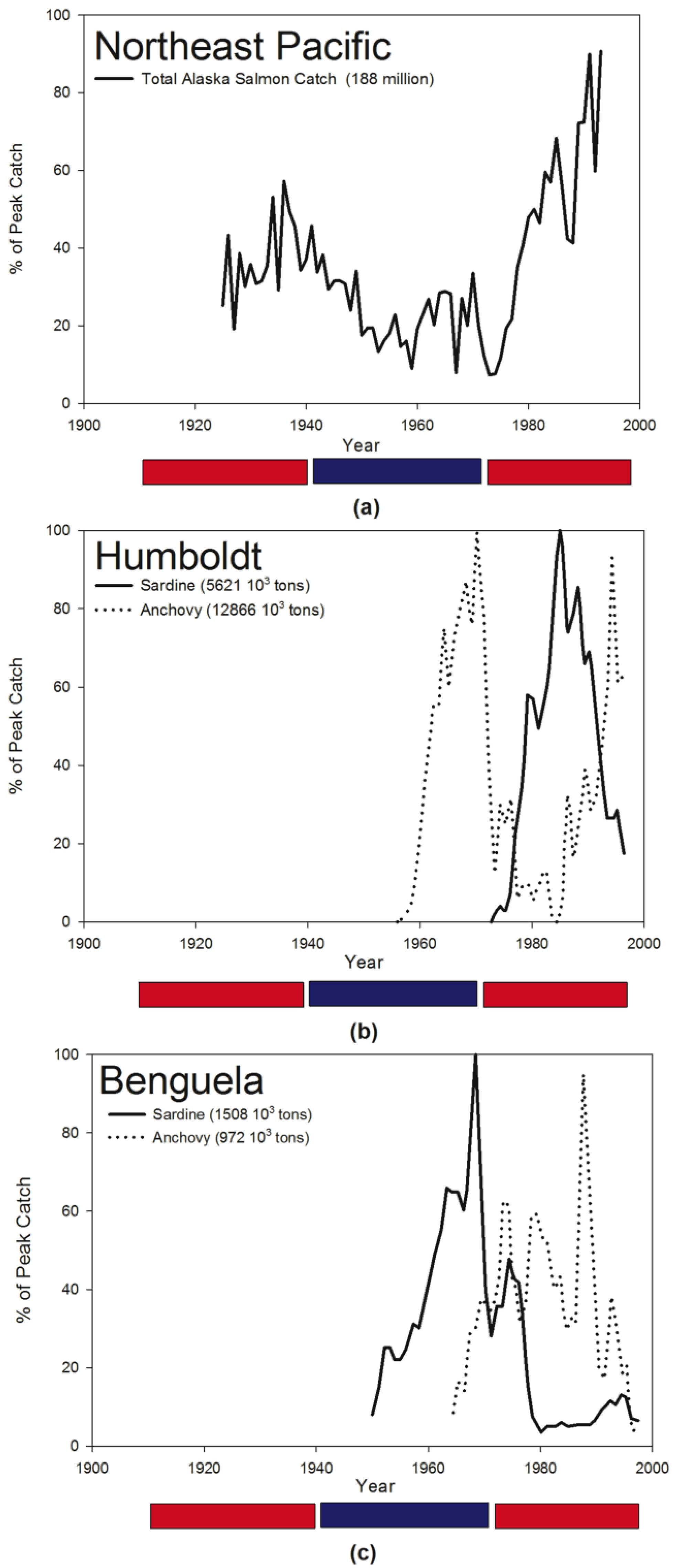
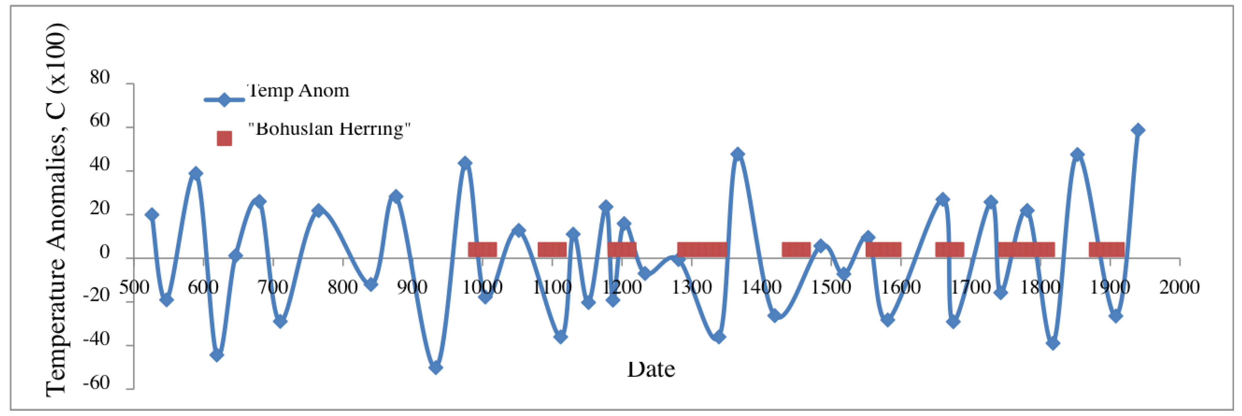
5. Alternations in Fish Populations

Along continental margins of the subtropical gyres, changes in upwelling and the resulting temperature and chlorophyll concentrations set the stage for alternating abundances of weak and strong upwelling phase preferring fish species (Figure 4). In the meridional phase, equator-ward wind and upwelling increase and temperatures decrease in the Pacific (Table 1). By contrast, in the Atlantic wind and upwelling decrease and temperatures warm (Table 1). Satellite derived sea surface temperature in the Humboldt and California upwelling areas cooled after 2000, suggesting enhanced upwelling (Figure 4a,b), consistent with the speeding up of Pacific subtropical gyre circulation in the meridional phase. Additionally during that time in those areas, chlorophyll concentrations increased (Figure 4c). By contrast where gyre circulations slowed in the Atlantic after 2000, temperatures warmed and chlorophyll concentration decreased in the Iberia/Canary and Benguela regions (Figure 4). The NASSA funded Massachusetts Institute of Technology (MIT) global ocean circulation model temperature output for the period of 1992 to 2012 showed the same pattern of warming in the Canary and Benguela Currents and cooling in the California and Humboldt Currents as the observed temperatures indicated (Figure 5). Satellite wind data from upwelling areas showed consistent trends with temperature and chlorophyll in early 2000s data (Table 1). Oyshio wind data indicated a slowing trend consistent with slowing subpolar gyre circulation.
Fish populations from landings records appear to exhibit the cycles associated with natural decadal jet stream westerly wind change, alternating gyre circulations and the alternating intensity of upwelling off continental margins although they have also been impacted by intense harvest pressures over the past 100 years (Figure 3, Figure 4, Figure 5 and Figure 6). During the zonal wind periods, subarctic gyre fish populations switch from cool to warm species in the northeast Atlantic [9,34,77] and all species of salmon increase in abundance in the Pacific Aleutian gyre [5] (Figure 6a). In the northwest Pacific anchovy and sardine regime shifts occur with anchovies growing depending on optimal temperatures [78]. Also during the zonal phase as Pacific subtropical gyre circulation relaxes, upwelling relaxes off the western margins of continents and warm species of fish like sardines replace cool species like anchovies. Temperature preference may be more of a correlation where certain prey may be available for sardine during weak upwelling, with usually warmer temperatures and for anchovy during strong upwelling, with usually cooler temperatures off the western margin of continents. In other regions with weaker upwelling like the Northwestern Pacific Oyashio and South Africa Agulhas extension regions, sardines and their favored prey of sardines occur during cooler conditions and anchovy and their favored prey of anchovy occur during warmer conditions [79,80]. The alternation in dominance of small pelagic species is consistent with the flow hypothesis of MacCall [81] in which periods of weak boundary current flow favor sardines and periods of strong flow and stronger upwelling favor anchovies. The best evidence of the ecological impact of phase changes in gyre circulations and upwelling intensities comes from salmon fisheries and small pelagic fish (Figure 6).
The increased sheer in the Gulf of Alaska gyre or Aleutian gyre after the mid 1970s mixed nutrients to the surface stimulating phytoplankton growth and subsequently zooplankton abundances. The ecological changes included an increase in ground fish and pollock recruitment and Pacific salmon catches in the Gulf of Alaska Gyre (Figure 6a). Due to increased predation from these fish, pandalid shrimp and capelin forage fish declined and correlated with a crash in piscivorous sea bird and marine mammal populations [82]. During this zonal wind, warming phase and the warming phase from the 1910s to the 1940s, landings from all species of salmon increased in the Aleutian gyre system to 1997 [5] (Figure 6a). These oscillating changes in salmon landings have been recorded in sediment data for hundreds of years [83].
As more water is pulled into the Gulf of Alaska Gyre during the zonal phase, increasing circulation, less wind blows down the California Current, decreasing its upwelling. Evidence of decreased upwelling during the zonal phase after the 1970s was observed as water in the California current warmed and freshened with reduced mixing [84]. Primary production, zooplankton, pelagic fish and seabirds all decreased, with zooplankton decreasing by 80% [85]. By contrast and as expected with decreased upwelling, the Pacific sardine population increased off California from 1977 to the early 1990s [48,86]. Counts of seabirds only began after 1987 but declined 90% from the few early records available. Since the late 1990s despite expectation of stronger upwelling along California, no strong evidence of an increased abundance of zooplankton or anchovy has been revealed in surveys [87,88].
During the zonal phase in the Humboldt Current, sardine catches increased and anchovy catches decreased [4,48] (Figure 6b). Increases of sardines occurred simultaneously in the Humboldt, California and Japan-Kuroshio-Oyashio in the 1930s and after the 1970s, indicating global correlations of abundance [3]. In the Humboldt Current, Alheit and Hagen [89] identified two sardine phases (1930s to 1950s, 1970s to 1990s) and three cool anchovy phases (1920s to 1930s, 1950s to1970s, 1990s to present), corresponding to shifts in the global oscillation.
In the Benguela current off South Africa, the relative dominance of anchovies and sardines are out of phase compared to Pacific upwelling areas [4,90] (Figure 6). The out of phase shifting in fish species between the subtropical Atlantic and Pacific provide evidence supporting the out of phase subtropical gyre circulations. The northern Benguela current was a sardine dominated system from the 1950s to the mid 1960s and peaked in 1962 with 11 million tons; the regime shifted to an anchovy dominated system until the early 1990s when the anchovy stock declined [58,80,89]. Since severe harvest pressures in the 1960s northern sardines have failed to recover and show no evidence of expected dominance in the early 2000s meriodional mode [58]. Currently both sardine and anchovy stocks remain low in the northern Benguela current.
Most of the fish landing data shown above come from short data sets from the mid 20th century. Thus mechanistic links between gyre circulation and fish species must be cautiously interpreted particularly in the light of lack of correlation for some species and areas due to perhaps, harvest pressure. One example to illustrate correlations for the long term is the Bohuslän Herring in the North Atlantic subpolar oscillation. The seine fishery for Bohuslän Herring from the North Sea off the south coast of Sweden was recorded from about the year 1000 to 1900 [91]. This unique data set of the cold preferring herring species displays maximum abundances generally during the cool portion of the cycles (Figure 7).
Figure 6. Fish landings of: (a) salmon in the Northeast Pacific; (b) sardines and anchovies in the Humboldt; and (c) anchovies and sardines in the Benguela current systems. Fish catch are given as the percent of peak catch of the time series, region specific. Values in figure legends represent the maximum landings of the fish catch over the time periods. The blue/red bars indicate the cool/warm phases over the last century. Data were adapted from Hare and Francis [92] (a), de Young et al. [93] (b,c). Species’ dominances are shown to change with the warm and cool phases. Species’ dominances are shown to change with the warm and cool phases which have been originally labeled NAO for Atlantic stocks and PDO/ Inderdecadal Pacific Oscillation (IPO) for Pacific stocks.
Climate 03 00833 g006
Figure 7. Temperature anomalies, °C, as in Figure 2 (×100) displayed with maximum abundances of Swedish Herring (arbitrary units) adapted from Alheit and Hagen [91].
Climate 03 00833 g007

6. The Future: Anthropogenic Climate Change

Several authors have indicated how wind oscillations may be altered as anthropogenic gases heat the earth’s troposphere, or deplete ozone, and as atmospheric water vapor concentrations change [94,95,96,97,98]. For example, as the greenhouse gases CO2 and CH4 accumulate in the troposphere and trap heat, the stratosphere is cooled, intensifying the westerly winds at both poles [94]. Global warming due to greenhouse gases apparently intensifies the positive phase of the cycle [95,96,97,98]. The recent zonal phase, of the westerly winds in the northern hemisphere from the 1970s to the 1990s, was the strongest NAO oscillation in the recorded record [17]. Freshening waters at the poles, warming of Atlantic intermediate waters, a warming, spreading Atlantic-derived sub-layer across the Arctic Eurasian basin, an increased Arctic ice efflux through the western Fram Strait over the same NAO period were deemed consistent with climate model predictions of the processes of global change [17]. Surface westerly winds in the southern hemisphere have shifted poleward and also intensified in the austral summer with the Antarctic ozone hole representing one possible explanation for the shift [96,97]. The westerly winds in the southern hemisphere have increased more than those in the northern hemisphere due possibly to ozone depletion [98]. The loss of ozone would cool the cold air over Antarctica increasing the thermal gradient between the pole and the tropics making the southern westerlies stronger. A poleward shift in the westerly winds whether due to a warming climate, increased ozone or natural fluctuation may decrease global warming and anthropogenic carbon dioxide increase in the atmosphere [99]. Russell et al. [100] suggest that the strength and latitude of the southern westerlies, that have shifted poleward and increased by 20% during the zonal period, have a large effect on the ability of the southern ocean to take up heat and carbon. The authors propose that strong westerly winds when more aligned with the Antarctic circumpolar current may slow rates of stratification, thereby increasing the storage of heat through increased mixing and slowing anthropogenic carbon dioxide through dilution with older, lower carbon dioxide released in upwelled waters [99,100]. Heat sequestration and atmospheric carbon dioxide dilution act as negative feedbacks on climate warming and form an active area of current research [35]. Solomon et al. [98] proposed that stratospheric water vapor is also a driver or maybe, reflects, decadal global surface climate change. These authors use a combination of observations and models to suggest that stratospheric water vapor was correlated to climate warming between 1980 and 2000 and to the flattening of global warming since early 2000s. The intensity of the recent switch to a meridional wind phase has also been attributed to enhanced Arctic warming. The darker surface waters of the melting Arctic region absorb more heat leading to a decreased latitudinal temperature gradient and a weakened polar vortex of westerly winds characterizing the meridional wind phase [101].
The popular media reports on the scientists’ prediction in the Intergovernmental Panel on Climate Change (IPCC) [102] tend to project smooth trends for temperature increase over time when regionally at least, variable rates of increase would be more accurate. The actual IPCC report details the more complex relationship between regional climate change and global mean change [102]. During the recent zonal wind phase, temperatures increased dramatically over northern temperate continents [8]. Global air temperatures increased 0.61 ºC overall during the 20th century [103], but during zonal wind periods, the temperatures increased 1 to 2 ºC (Figure 2). During the current meridional phase, regional temperatures have stayed high but the rate of winter increase has slowed (Figure 1). The oscillating regional temperature patterns may cause oscillatory behavior in the intensity of upwelling in eastern boundary currents, ice melt, sea level rise, patterns of droughts and floods, storm intensity, agricultural productivity, etc. Due to the westerly winds, heating of the oceans has not taken place uniformly along the latitudinal gradient. While the subarctic Atlantic has cooled in the last half of the twentieth century consistent with isolation by the westerly winds, the subtropical Atlantic has warmed [104]. The natural variability of the westerly winds may make regional anthropogenic warming apparently slow in the present meridional wind phase as some news articles have recently suggested [105,106].

7. Summary

The relationship of decadal jet stream wind patterns to gyre circulation in this review should be considered as hypotheses to be tested (Figure 3). In the 20th century the global scope of multidecadal climate oscillations are revealed in instrumented data and through proxy data, for several previous centuries. The objective of this review of natural climate oscillations was to describe possible linkages between jet stream winds, gyre circulations, upwelling and fish abundance. Several hypotheses, which address causes of the oscillation, were described although none have been fully accepted by the scientific community. A large literature supports the framework of climate variations in specific oceanic areas described here. Data, particularly satellite data, and model output support gyre circulations inferred from the literature. Oceanic pieces of the puzzle are being synthesized and it is becoming more common to consider whole gyres and comparisons of parallel areas in different oceans [34,48,107]. The literature, reviewed for many researchers over the past 50 years, has suggested that the climate and fish populations in upwelling regions oscillate between two states (Figure 3 and Figure 6). Oscillation changes in the wind and intensity of upwelling off the western margins of continents in subtropical gyres may help explain asynchronous sardine abundances in the northern Benguela Current and anchovy abundances in the Humboldt Current although harvest pressures have recently disrupted patterns in the Benguela Current [58]. The evidence suggests that secular-scale regional anthropogenic climate trends may act to enhance the zonal phase of the global oscillation and in turn, may mute the meridional phase. The recognition of gyre scale changes in ecology should improve the management of fisheries particularly in upwelling areas, stimulate the further development of ocean observing systems and the search for other large scale ecological patterns.

Acknowledgments

LS and MCM received partial support from the National Oceanic and Atmospheric Association (grant NA05NOS4781201). We thank Shuwen Zhang for providing the MIT global circulation model temperature output from 1992 to 2012. Several colleagues including Barbara Sullivan Watts, Caroline Rogers and Aimee Keller provided comments on the manuscript. We thank several outside reviewers for the enormous effort, detailed comments and literature expertise that clarified much of the information presented.

Author Contributions

Candace Oviatt wrote the article and is responsible for any incorrect materials. Leslie Smith prepared the materials on the North Atlantic Oscillation and Rhode Island air temperature graphs and provided expert editing. M. Conor McManus provided the figures on the Mann temperature variations and fish abundance and provided expert editing. Kim Hyde provided the figures with satellite data on upwelling areas, and temperature and chlorophyll trends in these areas.

Conflicts of Interest

The authors declare no conflicts of interest.

References

  1. Hurrell, J.W.; Dickson, R.R. Climate variability over the North Atlantic. In Marine Ecosystems and Climate Variation: The North Atlantic: A Comparative Perspective; Stenseth, N.C., Ottersen, G., Hurrell, J.W., Belgrano, A., Eds.; Oxford University Press: New York, NY, 2004; pp. 15–32. [Google Scholar]
  2. Woollings, T.; Hoskins, B.; Blackburn, M.; Berrisford, P. A new rossby wave—Breaking interpretation of the North Atlantic Oscillation. J. Atmos. Sci. 2008, 65, 609–626. [Google Scholar] [CrossRef]
  3. Mann, K.; Lazier, J.R.N. Variability in ocean circulation: Its biological consequences. In Dynamics of Marine Ecosystems: Biological-Physical Interactions in the Oceans, 3rd ed.; Wiley-Blackwell: Hoboken, NJ, USA, 2006; pp. 337–389. [Google Scholar]
  4. Klyashtorin, L.B. Climate Change and Long-Term Fluctuations of Commercial Catches—The Possibility of Forecasting; FAO Fisheries: Rome, Italy, 2001. [Google Scholar]
  5. Beamish, R.J.; Noakes, D.J.; McFarlane, G.A.; Klyashtorin, L.; Ivanov, V.V.; Kurashov, V. The regime concept and natural trends in the production of Pacific salmon. Can. J. Fish. Aquat. Sci. 1999, 56, 516–526. [Google Scholar] [CrossRef]
  6. Deser, C.; Phillips, A.S.; Hurrell, J.W. Pacific interdecadal climate variability: Linkages between the tropics and the North Pacific during boreal winter since 1900. J. Climate 2004, 17, 3109–3124. [Google Scholar] [CrossRef]
  7. Mantua, N.J.; Hare, S.R.; Zhang, Y.; Wallace, J.M.; Francis, R.C. A Pacific interdecadal climate oscillation with impacts on salmon production. Bull. Amer. Meteor. Soc. 1997, 78, 1069–1079. [Google Scholar] [CrossRef]
  8. Mann, M.E.; Zhang, Z.; Rutherford, S.; Bradley, R.S.; Hughes, M.K.; Shindell, D.; Ammann, C.; Faluvegi, G.; Ni, F. Global signatures and dynamical origins of the little ice age and the medieval climate anomaly. Science 2009, 326, 1256–1260. [Google Scholar] [CrossRef] [PubMed]
  9. Marshall, J.; Kushnir, Y.; Battisti, D.; Chang, P.; Czaja, A.; Dickson, R.; Hurrell, J.; McCartney, M.; Saravanan, R.; Visbeck, M. North Atlantic climate variability: Phenomena, impacts and mechanisms. Int. J. Climatol. 2001, 21, 1863–1898. [Google Scholar] [CrossRef] [Green Version]
  10. Climate and Global Dynamics Division of the National Center for Atmospheric Research. Available online: http://www.cgd.ucar.edu/cas/jhurrell/indices.html (accessed on 5 October 2015).
  11. Cushing, D.H. Climate and Fisheries; Academic Press: New York, NY, USA, 1982; p. 373. [Google Scholar]
  12. National Aeronautics and Space Administration. Datasets and Imagines. Available online: http://data.giss.nasa.gov/ (accessed on 5 August 2015).
  13. AMO (Atlantic Multidecadal Oscillation) Index. Available online: http://www.esri.noaa.gov/psd/data/timeseries/AMO/index.html (accessed on 5 October 2015).
  14. Yoder, J.A.; Doney, S.C.; Siegel, D.A.; Wilson, C. Study of marine ecosystems and biogeochemistry now and in the future: Examples of unique contributions from space. Oceanography 2010, 23, 104–117. [Google Scholar] [CrossRef]
  15. Thompson, D.W.J.; Lee, S.; Baldwin, M.P. Atmospheric processes governing the Northern Hemisphere Annular Mode/North Atlantic Oscillation. In The North Atlantic Oscillation—Climatic Significance and Environmental Impact; Hurrell, J.W., Kushnir, Y., Ottersen, G., Visbeck, M., Eds.; American Geophysical Union: Washington, DC, USA, 2003; pp. 81–112. [Google Scholar]
  16. Hall, A.; Visbeck, M. Synchronous variability in the southern hemisphere atmosphere, sea ice, and ocean resulting from the annular mode. J. Climate 2002, 15, 3043–3057. [Google Scholar] [CrossRef]
  17. Dickson, R.R.; Hurrell, J.; Bindoff, N.; Wong, A.; Arbic, B.; Owens, W.B.; Imawaki, S.; Yashayaev, I. The world during WOCE. In Ocean Circulation and Climate—Observing and Modeling the Global Ocean; Siedler, G., Church, J., Gould, J., Eds.; Academic Press: New York, NY, USA, 2001; pp. 557–583. [Google Scholar]
  18. Francis, J.A.; Vavrus, S.J. Evidence linking Arctic amplification to extreme weather in mid-latitudes. Geophys. Res. Lett. 2012, 39. [Google Scholar] [CrossRef]
  19. Wallace, J.M.; Held, I.M.; Thompson, D.W.J.; Trenberth, K.E.; Walsh, J.E. Global warming and winter weather. Science 2014, 343, 729–730. [Google Scholar] [CrossRef] [PubMed]
  20. Scaife, A.A.; Knight, J.R.; Vallis, G.K.; Folland, C.K. A stratospheric influence on the winter NAO and North Atlantic surface climate. Geophys. Res. lett. 2005. [Google Scholar] [CrossRef]
  21. Minobe, S.; Kuwano-Yoshida, A.; Komori, N.; Xie, S.; Small, R.J. Influence of the Gulf Stream on the troposphere. Nature Lett. 2008, 452, 206–209. [Google Scholar] [CrossRef] [PubMed]
  22. Schimanke, S.; Korper, J.; Spangehl, T.; Cubasch, U. Multidecadal variability of sudden stratospheric warmings in the AOGCM. Geophys. Res. Lett. 2011, 38. [Google Scholar] [CrossRef]
  23. Omrani, N.; Keenlyside, N.; Bader, J.; Manzini, E. Stratosphere key for wintertime atmospheric response to warm Atlantic decadal conditions. Climate Dyn. 2014, 42, 649–663. [Google Scholar] [CrossRef]
  24. Thompson, D.W.J.; Lorenz, D.J. The signature of the annular modes in the tropical troposphere. J. Climate 2004, 17, 4330–4324. [Google Scholar] [CrossRef]
  25. Fogt, R.L.; Perlwitz, J.; Monaghan, A.J.; Bromwich, D.H.; Jones, J.M.; Marshall, G.J. Historical SAM variability. Part II: Twentieth-century variability and trends from reconstructions, observations, and IPCC AR4 models. J. Climate 2009, 22, 5346–5365. [Google Scholar] [CrossRef]
  26. Yuan, X.; Yonekura, E. Decadal variability in the southern hemisphere. J. Geophys. Res. 2011, 116. [Google Scholar] [CrossRef]
  27. Vangenheim, G. The long-term temperature and ice break-up forecasting. Proc. State Hydrol. Inst. Issue 1940, 10, 207–236. (In Russian) [Google Scholar]
  28. Kravtsov, S.; Wyatt, M.G.; Curry, J.A.; Tsonis, A.A. Two contrasting views of multidecadal climate variability in the twentieth century. Geophys. Res. Lett. 2014, 41, 6881–6888. [Google Scholar] [CrossRef]
  29. Girs, A.A. Multiyear Oscillations of Atmospheric Circulation and Long-term Meteorological Forecasts; Gidrometeroizdat: Moskva, Russia, 1971; p. 480. (In Russian) [Google Scholar]
  30. Overland, J.E.; Alheit, J.; Bakun, A.; Hurrell, J.W.; Mackas, D.L.; Miller, A.J. Climate controls on marine ecosystems and fish populations. J. Mar. Syst. 2010, 79, 305–315. [Google Scholar] [CrossRef]
  31. Hurrell, J. North Atlantic oscillation. In Climate and Oceans—A Derivative of the Encyclopedia of Ocean Sciences, 2nd ed.; Steele, J., Thorpe, S., Turekian, K., Eds.; Elsevier: New York, NY, USA, 2010; pp. 33–40. [Google Scholar]
  32. Knight, J.R.; Folland, C.K.; Scarife, A.A. Climate impacts of the Atlantic Multidecadal Oscillation. Geophys. Res. Lett. 2006, 33. [Google Scholar] [CrossRef]
  33. Mann, M.E. The Hockey Stick and the Climate Wars: Dispatches from the Front Lines; Columbia University Press: New York, NY, USA, 2012. [Google Scholar]
  34. Nye, J.A.; Baker, M.R.; Bell, R.; Kenny, A.; Kilbourne, K.H.; Friedland, K.D.; Martino, E.; Strachura, M.M.; Van Houtan, K.S.; Wood, R. Ecosystem effects of the Atlantic Multidecadal Oscillation. J. Mar. Syst. 2013, 133, 103–116. [Google Scholar] [CrossRef]
  35. Chen, X.; Tung, K.-K. Varying planetary heat sink led to global-warming slowdown and acceleration. Science 2014, 345, 897–903. [Google Scholar] [CrossRef] [PubMed]
  36. Broeker, W. The Great Ocean Conveyor: Discovering the Trigger for Abrupt Climate Change; Princeton University Press: Princeton, NJ, USA, 2010. [Google Scholar]
  37. Manabe, S.; Stouffer, R.J. Two stable equilibria of a coupled ocean-atmosphere model. J. Climate 1988, 1, 841–866. [Google Scholar] [CrossRef]
  38. Lozier, M.S. Deconstructing the conveyor belt. Science 2012, 328, 1507–1511. [Google Scholar] [CrossRef] [PubMed]
  39. Srokosz, M.A.; Bryden, H.L. Observing the Atlantic meridional overturning circulation yields a decade of inevitable surprises. Science 2015, 348. [Google Scholar] [CrossRef] [PubMed]
  40. Seidov, D.; Haupt, B.J.; Barron, E.J.; Maslin, M. Ocean bi-polar seesaw and climate: Southern versus northern meltwater impacts. In The Oceans and Rapid Climate Change: Past Present and Future; Seidov, D., Haupt, B.J., Maslin, M., Eds.; AGU: Washington, DC, USA, 2001; pp. 169–197. [Google Scholar]
  41. Rahmstorf, S. Ocean circulation and climate during the past 120,000 years. Nature 2002, 419, 207–214. [Google Scholar] [CrossRef]
  42. Kilbourne, K.H.; Quinn, T.M.; Guilderson, T.P.; Webb, R.S.; Taylor, F.W. Decadal- to interannual-scale source water variations in the Caribbean Sea recorded by Puerto Rican coral radiocarbon. Climate Dyn. 2007, 29, 51–62. [Google Scholar] [CrossRef]
  43. Garzoli, S.; Matano, R. The South Atlantic and the Atlantic meridional overturning circulation. Deep Sea Res. Part II Top.Stud. Oceanogr. 2011, 1158, 1837–1847. [Google Scholar] [CrossRef]
  44. Broecker, W.S.; Sutherland, S.; Peng, T. A possible 20th century slowdown of southern ocean deep water formation. Science 1999, 286, 1132–1135. [Google Scholar] [CrossRef] [PubMed]
  45. Ganachaud, A.; Wunsch, C. Improved estimates of global ocean circulation, heat transport and mixing from hydrographic data. Lett. Nature 2000, 408, 453–457. [Google Scholar] [CrossRef] [PubMed]
  46. Hayes, C.T.; Marinez-Garcia, A.; Hasenfratz, A.P.; Jaccard, S.L.; Hodell, D.A.; Sigman, D.M.; Haug, G.H.; Anderson, R.F. A stagnation event in the deep South Atlantic during the last interglacial period. Science 2014, 346, 1514–1516. [Google Scholar] [CrossRef] [PubMed] [Green Version]
  47. Wyatt, M.G.; Curry, J.A. Role for Eurasian Arctic shelf sea ice in a secularly varying hemispheric climate signal during the 20th century. Climate Dyn. 2014, 42, 2763–2782. [Google Scholar] [CrossRef]
  48. Chavez, F.P.; Ryan, J.; Lluch-Cota, S.E.; Niquen, M. From anchovies to sardines and back: Multidecadal change in the Pacific Ocean. Science 2003, 299, 217–221. [Google Scholar] [CrossRef] [PubMed]
  49. Xie, S.-P.; Carton, J.A. Tropical Atlantic variability: Patterns, mechanisms, and Impacts. In Earth Climate: The Ocean-Atmosphere Interaction Geophysical Monograph; Wang, C., Xie, S.P., Carton, J.A., Eds.; AGU: Washington, DC, USA, 2004; pp. 121–142. [Google Scholar]
  50. Curry, R.G.; McCartney, M.S. Ocean gyre circulation changes associated with the North Atlantic Oscillation. J. Phys. Oceanogr. 2001, 31, 3374–3400. [Google Scholar] [CrossRef]
  51. Yashayaev, I.; Dickson, B. Transformation and fate of overflows in the Northern North Atlantic. In Arctic-Subarctic Ocean Fluxes; Dickson, R.R., Meincke, J., Rhines, P., Eds.; Springer: Dordrecht, The Netherlands, 2008; pp. 505–526. [Google Scholar]
  52. Oviatt, C. The changing ecology of temperate coastal waters during a warming trend. Estuaries 2004, 27, 895–904. [Google Scholar] [CrossRef]
  53. Visbeck, M.; Chassignet, E.; Curry, R.; Delworth, T.; Dickson, R.; Krahmann, G. The ocean’s response to North Atlantic Oscillation variability. In The North Atlantic Oscillation: Climatic Significance and Environmental Impact; Hurrell, J.W., Kushnir, Y., Ottersen, G., Visbeck, M., Eds.; American Geophysical Union: Washington, DC, USA, 2003; pp. 113–145. [Google Scholar]
  54. Hakkinen, S.; Hatun, H.; Rhines, P. Satellite evidence of change in the northern gyre. In Arctic-Subarctic Ocean Fluxes Defining the Role of the Northern Seas in Climate; Dickson, R., Meincke, J., Rhines, P., Eds.; Springer: Dordrecht, The Netherlands, 2008; pp. 551–567. [Google Scholar]
  55. Häkkinen, S.; Rhines, P.B.; Worthen, D.L. Atmospheric blocking and Atlantic multidecadal ocean variability. Science 2011, 334, 655–659. [Google Scholar] [CrossRef] [PubMed]
  56. Venegas, S.; Mysak, L.; Straub, D. Evidence for interannual and interdecadal climate variability in the South Atlantic. Geophys. Res. Lett. 1996, 23, 2673–2676. [Google Scholar] [CrossRef]
  57. Emeis, K.-C.; Struck, U.; Leipe, T.; Ferdelman, T.G. Variability in upwelling intensity and nutrient regime in the coastal upwelling system offshore Namibia: Results from sediment archives. Int. J. Earth Sci. 2009, 98, 309–326. [Google Scholar] [CrossRef]
  58. Kreiner, A.; Yemane, D.; Stenevik, E.; Moroff, N. The selection of spawning location of sardine (Sardinops sagax) in the northern Benguela after changes in stock structure and environmental conditions. Fish. Oceanogr. 2001, 20, 560–569. [Google Scholar] [CrossRef]
  59. Hutchings, L.; van der Lingen, C.D.; Shannon, L.J.; Crawford, R.J.M.; Verheye, H.M.S.; Bartholomae, C.H.; van der Plas, A.K.; Louw, D.; Kreiner, A.; Ostrowski, M.; et al. The Benguela Current: An ecosystem of four components. Prog. Oceanogr. 2009, 83, 15–32. [Google Scholar] [CrossRef]
  60. Verheye, H.M. Decadal-scale trends across several marine trophic levels in the southern Benguela upwelling system off South Africa. AMBIO A J. Hum. Environ. 2000, 29, 30–34. [Google Scholar] [CrossRef]
  61. Daskalov, G.; Boyer, D.; Roux, J. Relating sardine Sardinops sagax abundance to environmental indices in northern Benguela. Prog. Oceanogr. 2003, 59, 257–274. [Google Scholar] [CrossRef]
  62. Wainer, I.; Venegas, S. South Atlantic multidecadal variability in the climate system model. J. Climate. 2002, 15, 1408–1420. [Google Scholar] [CrossRef]
  63. Clarke, A.; Lebedev, A. Remotely driven decadal and longer changes in the coastal Pacific waters of the Americas. J. Phys. Oceanogr. 1999, 29, 828–835. [Google Scholar] [CrossRef]
  64. McPhaden, M.; Zebiak, S.; Glantz, M. ENSO as an integrating concept in earth science. Science 2006, 314, 1740–1745. [Google Scholar] [CrossRef] [PubMed]
  65. Euler, C.; Ninnemann, U. Climate and Antarctic intermediate water coupling during the late Holocene. Geology 2010, 38, 647–650. [Google Scholar] [CrossRef]
  66. O’Kane, T.J.; Risbey, J.S.; Franzke, C.; Horenko, I.; Monselesan, D.P. Changes in the metastability of the midlatitude Southern Hemisphere circulation and the utility of nonstationary cluster analysis and split-flow blocking indices as diagnostic tools. J Atmos. Sci. 2013, 70, 824–842. [Google Scholar] [CrossRef]
  67. O’Kane, T.J.; Matear, R.J.; Chamberlain, M.A.; Oke, P.R. ENSO regimes and the late 1970’s climate shift: The role of synoptic weather and South Pacific ocean spiciness. J. Comput. Phys. 2014, 271, 19–38. [Google Scholar] [CrossRef]
  68. Chhak, K.; Di Lorenzo, E. Decadal variations in the California current upwelling cells. Geophys. Res. Lett. 2007, 34. [Google Scholar] [CrossRef]
  69. Di Lorenzo, E.; Schneider, N.; Cobb, K.; Franks, P.; Chhak, K.; Miller, A.; McWilliams, J.; Bograd, S.; Arango, H.; Curchitser, E.; et al. North Pacific gyre oscillation links ocean climate and ecosystem change. Geophys. Res. Lett. 2008, 35. [Google Scholar] [CrossRef]
  70. Casey, K.S.; Brandon, T.B.; Cornillon, P.; Evans, R. The past, present and future of the AVHRR pathfinder SST program. In Oceanography from Space; Barale, V., Gower, J.F.R., Alberotanza, L., Eds.; Springer: Dordrecht, The Netherlands, 2010; pp. 273–287. [Google Scholar]
  71. OceanColor Web. Available online: http://oceancolor.gsfc.nasa.gov/cms/ (accessed on 15 July 2015).
  72. Chavez, F.; Messier, M. A comparison of eastern boundary upwelling ecosystems. Prog. Oceanogr. 2009, 83, 80–96. [Google Scholar] [CrossRef]
  73. Curry, P.; Shannon, L. Regime shifts in upwelling ecosystems: Observed changes and possible mechanisms in northern and southern Benguela. Prog. Oceanogr. 2004, 60, 223–243. [Google Scholar] [CrossRef]
  74. Alheit, J.; Niqven, M. Regime shifts in the Humboldt Current ecosystem. Prog. Oceanogr. 2004, 60, 201–222. [Google Scholar] [CrossRef]
  75. Field, D.; Baumgartner, T.; Ferreira, V.; Gutierrez, D.; Lozano-Montes, H.; Salvatteci, R.; Soutar, A. Variability from scales in marine sediments and other historical records. In Climate Change and Small Pelagic Fish; Checkley, D.M., Jr., Alheit, J., Oozeki, Y., Roy, C., Eds.; Cambridge University Press: Cambridge, UK, 2009; pp. 45–63. [Google Scholar]
  76. Roemmich, D.; Gilson, J.; Davis, R.; Sutton, P.; Wijffels, S.; Riser, S. Decadal spin up of the South Pacific substropical gyre. J. Phys. Oceanogr. 2007, 37, 162–173. [Google Scholar] [CrossRef]
  77. Drinkwater, K.; Belgrano, A.; Borja, A.; Conversi, A.; Edwards, M.; Greene, C.; Ottersen, G.; Pershing, A.; Walker, H. The response of marine ecosystems to climate variability associated with the North Atlantic oscillation. In The North Atlantic Oscillation—Climatic Significance and Environmental Impact; Hurrell, J., Kushnir, Y., Ottersen, G., Visbeck, M., Eds.; American Geophysical Union: Washington, DC, USA, 2003; pp. 211–234. [Google Scholar]
  78. Takasuka, A.; Oozed, Y.; Aoki, I. Optimal growth temperature hypothesis: Why do anchovy flourish and sardine collapse or vice versa under the same ocean regime? Can. J. Fish. Aquat. Sci. 2007, 64, 768–776. [Google Scholar] [CrossRef]
  79. Takasuka, A.; Oozeki, Y.; Kubota, H.; Lluch-Cota, S. Contrasting spawning temperature optima: Why are anchovy and sardine regime shifts synchronous across the North Pacific? Prog. Oceanogr. 2008, 77, 225–232. [Google Scholar] [CrossRef]
  80. van der Lingen, C.; Hutchings, L.; Merkle, D.; van der Westhuizen, J.; Nelson, J. Comparative spawning habitats of anchovy (Engraulis capensis) and sardine (Sardinops sagax) in the southern Benguela upwelling ecosystem. In Spatial Processes and Management of Marine Populations; Kruse, G., Bez, N., Booth, T., Dorn, M., Hills, S., Lipcius, R., Pelletier, D., Roy, C., Smith, S., Witherell, D., Eds.; University of Alaska Sea Grant: Fairbanks, AK, USA, 2001; pp. 185–209. [Google Scholar]
  81. MacCall, A. Mechanisms of low-frequency fluctuations in sardine and anchovy populations. In Climate Change and Small Pelagic Fish; Checkley, D., Jr., Alheit, J., Oozeki, Y., Roy, C., Eds.; Cambridge University Press: Cambridge, UK, 2009; pp. 285–299. [Google Scholar]
  82. Anderson, P.; Piatt, J. Community reorganization in the Gulf of Alaska following ocean climate regime shift. Mar. Ecol. Prog. Ser. 1999, 189, 117–123. [Google Scholar] [CrossRef]
  83. Gregory-Eaves, I.; Selbie, D.; Sweetman, J.; Finney, B.; Smol, J. Tracking sockeye salmon population dynamics from lake sediment cores: A review and synthesis. Am. Fish. Soc. Symp. 2009, 69, 379–393. [Google Scholar]
  84. McGowan, J.; Cayan, D.; Dorman, L. Climate-ocean variability and ecosystem response in the Northeast Pacific. Science 1998, 281, 210–217. [Google Scholar] [CrossRef] [PubMed]
  85. Roemmich, D.; McGowan, J. Climate warming and the decline of zooplankton in the California current. Science 1995, 267, 1324–1326. [Google Scholar] [CrossRef] [PubMed]
  86. King, J.; Agostini, V.; Harvey, C.; McFarlane, G.; Foreman, M.; Overland, J.; Di Lorenzo, E.; Bond, N.; Aydin, K. Climate forcing and the California Current ecosystem. ICES J. Mar. Sci. 2011, 68, 1199–1216. [Google Scholar] [CrossRef]
  87. Lavaniegos, B.E.; Ohman, M.D. Coherence of long-term variations of zooplankton in two sectors of the California Current System. Prog. Oceanogr. 2007, 75, 42–69. [Google Scholar] [CrossRef]
  88. Ralston, S.; Field, J.C.; Sakuma, K.M. Long-term variation in a central California pelagic forage assemblage. J. Mar. Syst. 2015, 146, 26–37. [Google Scholar] [CrossRef]
  89. Alheit, J.; Hagen, E. The effect of climatic variation on pelagic fish and fisheries. In History and Climate—Memories of the Future; Jones, P., Ogilvie, A., Davies, T., Briffa, K., Eds.; Kluwer Academic/Plenum Publishers: New York, NY, USA, 2001; pp. 247–265. [Google Scholar]
  90. Lluch-Belda, D.; Schwartzlose, R.; Serra, R.; Parrish, R.; Kawasaki, T.; Hedgecock, D.; Crawford, R. Sardine and anchovy regime fluctuations of abundance in four regions of the world oceans: A workshop report. Fish. Oceanogr. 1992, 1, 339–347. [Google Scholar] [CrossRef]
  91. Alheit, J.; Hagen, E. Long-term climate forcing of European herring and sardine populations. Fish. Oceanogr. 1997, 6, 130–139. [Google Scholar] [CrossRef]
  92. Hare, S.R.; Francis, R.C. Climate change and salmon production in the Northeast Pacific Ocean. In Climate Change and Northern Fish Populations; Beamish, R.J., Ed.; NRC Research Press: Ottawa, ON, Canada, 1995; pp. 357–372. [Google Scholar]
  93. de Young, B.; Harris, R.; Alheit, J.; Beaugrand, G.; Mantua, N.; Shannon, L. Detecting regime shifts in the ocean: Data considerations. Prog. Oceanogr. 2004, 60, 143–164. [Google Scholar] [CrossRef]
  94. Shindell, D.; Schmidt, G.; Miller, R.; Rind, D. Northern Hemisphere winter climate response to greenhouse gas, volcanic, ozone and solar forcing. J. Geophys. Res. 2002, 106, 7193–7210. [Google Scholar] [CrossRef]
  95. Knutson, T.; Manabe, S. Assessment of decadal variability and trends in the tropical Pacific Ocean. J. Climate. 1998, 11, 2273–2296. [Google Scholar] [CrossRef]
  96. Lee, S.; Feldstein, S. Detecting ozone- and greenhouse gas-driven wind trends with observational data. Science 2013, 339, 563–567. [Google Scholar] [CrossRef] [PubMed]
  97. Waugh, D.; Primeau, F.; DeVries, T.; Holzer, M. Recent changes in the ventilation of the Southern Ocean. Science 2013, 339, 568–570. [Google Scholar] [CrossRef] [PubMed]
  98. Solomon, S.; Rosenlof, K.; Portmann, R.; Daniel, J.; Davis, S.; Sanford, T.; Plattner, G.K. Contributions of stratospheric water vapor to decadal changes in the rate of global warming. Science 2010, 327, 1219–1223. [Google Scholar] [CrossRef] [PubMed]
  99. Toggweiler, J.; Russell, J. Ocean circulation in a warming climate. Nature 2008, 451, 286–288. [Google Scholar] [CrossRef] [PubMed]
  100. Russell, J.; Dixon, K.; Gnanadesikan, A.; Stouffer, R.; Toggweiler, J. The Southern Hemisphere Westerlies in a warming world: Propping open the door to the deep ocean. J. Climate 2006, 19, 6382–6390. [Google Scholar] [CrossRef]
  101. Greene, C.; Monger, B. An Arctic wild card in the weather. Oceanography 2012, 25, 7–9. [Google Scholar] [CrossRef]
  102. Intergovernmental Panel on Climate Change (IPCC). Summary for policy makers. In Climate Change 2007: Impacts, Adaptation and Vulnerability. Contribution of Working Group II to the Fourth Assessment Report of the Intergovernmental Panel on Climate Change; Parry, M.L., Canziani, O.F., Palutikof, J.P., van der Linden, P.J., Hanson, C.E., Eds.; Cambridge University Press: Cambridge, UK, 2007; pp. 7–22. [Google Scholar]
  103. Folland, C.; Karl, T.; Salinger, M. Observed climate variability and change. Weather 2002, 57, 269–278. [Google Scholar] [CrossRef]
  104. Lozier, M.; Leadbetter, R.; Williams, S.; Roussenov, V.; Reed, M.; Moore, N. The spatial pattern and mechanisms of heat content change in the North Atlantic. Science 2008, 319, 800–803. [Google Scholar] [CrossRef] [PubMed]
  105. Kerr, R. What happened to global warming? Scientists say just wait a bit. Science 2009, 326, 28–29. [Google Scholar] [CrossRef] [PubMed]
  106. Trenberth, K. Has there been a hiatus? Internal climate variability masks climate-warming trends. Science 2015, 349, 691–692. [Google Scholar] [CrossRef] [PubMed]
  107. Sydeman, W.; Garcia-Reyes, M.; Scoheman, D.; Rykaczewski, R.; Thompson, S.; Black, B.; Bograd, S. Climate change and wind intensification in coastal upwelling ecosystems. Science 2014, 345, 77–80. [Google Scholar] [CrossRef] [PubMed]

