Abstract
Evapotranspiration (ET) and sensible heat (H) flux play a critical role in climate change; micrometeorology; atmospheric investigations; and related studies. They are two of the driving variables in climate impact(s) and hydrologic balance dynamics. Therefore, their accurate estimate is important for more robust modeling of the aforementioned relationships. The Bowen ratio energy balance method of estimating ET and H diffusions depends on the assumption that the diffusivities of latent heat (KV) and sensible heat (KH) are always equal. This assumption is re-visited and analyzed for a subsurface drip-irrigated field in south central Nebraska. The inequality dynamics for subsurface drip-irrigated conditions have not been studied. Potential causes that lead KV to differ from KH and a rectification procedure for the errors introduced by the inequalities were investigated. Actual ET; H; and other surface energy flux parameters using an eddy covariance system and a Bowen Ratio Energy Balance System (located side by side) on an hourly basis were measured continuously for two consecutive years for a non-stressed and subsurface drip-irrigated maize canopy. Most of the differences between KV and KH appeared towards the higher values of KV and KH. Although it was observed that KV was predominantly higher than KH; there were considerable data points showing the opposite. In general; daily KV ranges from about 0.1 m2∙s−1 to 1.6 m2∙s−1; and KH ranges from about 0.05 m2∙s−1 to 1.1 m2∙s−1. The higher values for KV and KH appear around March and April; and around September and October. The lower values appear around mid to late December and around late June to early July. Hourly estimates of KV range between approximately 0 m2∙s−1 to 1.8 m2∙s−1 and that of KH ranges approximately between 0 m2∙s−1 to 1.7 m2∙s−1. The inequalities between KV and KH varied diurnally as well as seasonally. The inequalities were greater during the non-growing (dormant) seasons than those during the growing seasons. During the study period, KV was, in general, lesser than KH during morning hours and was greater during afternoon hours. The differences between KV and KH mainly occurred in the afternoon due to the greater values of sensible heat acting as a secondary source of energy to vaporize water. As a result; during the afternoon; the latent heat diffusion rate (KV) becomes greater than the sensible heat diffusion rate (KH). The adjustments (rectification) for the inequalities between eddy diffusivities is quite essential at least for sensible heat estimation, and can have important implications for application of the Bowen ratio method for estimation of diffusion fluxes of other gasses.
1. Introduction
Accurate estimation of evapotranspiration (ET) is an essential as well as challenging task to scientists, researchers, and water managers. Bowen Ratio Energy Balance (BREB) and Eddy Covariance (EC) methods are probably most widely used to quantify in-field ET rates for a variety of vegetated and non-vegetated surfaces in research settings [1]. Similar to other procedures, BREB and EC methods also function based on some assumptions. For example, EC method depends on the turbulent mixing of atmospheric gases while BREB method depends on two major assumptions—(i) equality between eddy diffusivities of sensible heat and latent heat; and (ii) complete closure of terrestrial energy balance equation. However, depending on environmental factors, including the physical, biophysical, and boundary layer characteristics of the evaporating surface and the surrounding environment, the similarity assumption may not always be valid. In this study, the dynamics involved only with the first assumption was investigated.
The Bowen ratio method [2] is a practical application of Fick’s law of diffusion. In Fick’s law, the diffusivities of sensible heat (KH) and that of latent heat (KV) appear as proportionality constants. To avoid the practical difficulties of measuring actual values of KV and KH, the Bowen ratio method assumes that they are numerically equal to each other all the time. The theoretical aspects of the Bowen ratio method will be discussed later. The assumption of equality between KV and KH is an application of similarity hypothesis [3], which assumes that since both sensible heat and latent heat are carried out by the same parcel of air, the diffusivities can be considered to be equal. However, the application of similarity hypothesis of Monin and Obukov or the assumption KV = KH in the Bowen ratio theory may not hold for some conditions [1,4,5,6,7,8,9,10,11,12,13] and violating this assumption may result in errors in the estimated ET rates. The comparative analysis between KV and KH for various surfaces is a continuous topic of research among scientists. For example while some scientists have argued that KH is higher than KV [1,7,11,13], others have argued the opposite [5,9,14]. From their theoretical analyses, authors in [12] reported that the equality between KV and KH depends heavily on the correlation between the fluctuations of air temperature and humidity. A similar result was observed experimentally by [9], who theoretically showed that the ratio of KH to KV is simply the ratio of flux Bowen ratio (estimated by eddy covariance method) to gradient Bowen ratio (estimated by Bowen ratio energy balance method). The latter concept has been used by other researchers [6,7,8]. The authors in [9] also pointed out that advection might cause KV to substantially differ from KH. The authors in [6] used the later concept and estimated the ratio of KV to KH by separating the source of advective and non-advective fluxes. The authors in [15] showed that the ratio of KV to KH can be estimated by considering the sum and the difference of latent heat and sensible heat as the two separate energy variables, diffusing as proportional to the sum and difference, respectively, of moisture gradient and temperature gradient. The authors in [7] argued that difference between KV and KH are caused by several physical and atmospheric factors, small and large scale disturbances below and above the boundary layer. The authors in [8] empirically estimated the ratio of KV to KH using several micrometeorological variables as the regressors. More recently, two diffusivities were empirically estimated as a function of Richardson number [1].
An assumption of equality between KV and KH may, most likely, produce some errors in ET estimations. Nevertheless, often BREB system, which assumes the equality between KV and KH, is used in water management practices because of its cost effectiveness and ease of maintenance. While it is shown that the equality assumption may not hold for different vegetation surfaces under various microclimatic-surface-boundary layer interactions, justifying further investigation, the inequalities in energy coefficients for subsurface drip-irrigated maize canopy have not been studied. Irrigation and other management conditions can be particularly important and influential to the equality dynamics between KV and KH as the diffusivities and the equality assumptions could be affected by the degree and type of surface wetting (irrigation regime, i.e., sprinkler irrigation versus subsurface drip irrigation). Sprinkler irrigation systems wet both plant and soil surface resulting in increased soil evaporation and altering the microclimate of the plant and soil community, which in turn, can influence the relationship between KV and KH, especially in the lower canopy profile [16]. The main objective with this research is to further investigate the dynamics involved in the inequality between KV and KH for a subsurface drip irrigated and non-stressed maize (Zea mays L.) canopy and to develop a rectification procedure for the errors introduced by the inequalities.
2. Theoretical Synopses
2.1. Law of Turbulent Diffusion
The Bowen ratio method of estimating ET [2] is basically a modification of the law of turbulent diffusion. The law quantifies the amount of diffusion flux of an entity in the perpendicular direction a plane as proportional to the gradient of that same entity on both sides of the plane. Therefore, ET or moisture flux in a vertical direction can be expressed as:
where,
is ET represented in units of energy
is the coefficient of latent heat for water vapor),
is the moisture gradient in the vertical direction (z), and
is the eddy diffusivity for latent heat. Similarly, sensible heat (H) diffusion in a vertical direction can be written as:
where,
is the specific temperature gradient in the vertical direction and
is the eddy diffusivity for sensible heat. The negative signs in both Equations (1) and (2) represent directions, which means when the concentration increases in a vertically downward direction the positive diffusion flux is directed vertically upward. Also, from Equation (1) it is evident that
can be defined as the latent heat diffusion rate per unit moisture gradient. Similarly, from Equation (2) it is evident that
can be defined as the sensible heat diffusion rate per unit of temperature gradient.
2.2. Theory of Bowen Ratio
Author in [2] intended to develop a procedure to estimate water loss by evaporation from lakes using some easily measurable micrometeorological parameters. He primarily estimated the ratio of sensible heat to latent heat and used that ratio in an equation similar to the energy balance equation to estimate
or H. He first established that specific latent heat is directly proportional to the difference of vapor pressure between the two heights, and specific sensible heat is directly proportional to the difference of specific temperature between the two heights. By applying these concepts to the diffusion Equation (Equations (1) and (2)), with an assumption that the wind speed is a function of height, he developed the following partial differential equations for the latent heat flux and sensible flux diffusions:
where, θ and φ represent specific sensible and specific latent heat per unit volume, respectively, and f(z) is the wind speed as a function of height z.
In the field environment it is extremely difficult to estimate KV and KH accurately. Therefore, Bowen ratio method bypasses this difficulty by estimating the ratio of H to
(Bowen ratio) from relatively easily measureable atmospheric variables and substituting the ratio into the energy balance equation (Equation (5)). The most commonly used practical equations for estimating
and H fluxes in the vertical direction, using Bowen ratio method, are given in Equations (6) and (7), respectively:
where, Rn is net radiation, G is soil heat flux, P is air pressure, Cp is thermal heat capacity of air,
is air density,
is temperature gradient in a vertical direction, and
is the vapor pressure gradient in a vertical direction. The equality assumption assumes that the ratio (KH/KV) is equal to unity.
2.3. Theory of Eddy Covariance Method
The eddy covariance method is considered to be a direct approach of estimating sensible or latent heat diffusion. Originally developed by [17], eddy covariance approach relies on turbulent mixing of atmospheric gases. During turbulent transport, the transport of heat takes place through rapidly circulating air masses, known as eddies. Eddies can vary in dimensions with smaller eddies generated by small scale regions and larger eddies generated by larger areas. In general, the eddy covariance method relies on the concepts of instantaneous fluctuations of atmospheric variables inside a parcel of air or an eddy, and on the concepts of the heat flow through an isobaric surface. The author in [18] slightly advanced this concept to make it more applicable for the practical purpose, and gave a first instrumental demonstration of practical application of eddy covariance method. The modern day eddy covariance λE and H estimation procedures basically follow Swinbank’s approach. The latent heat and sensible heat, respectively, can be estimated by eddy covariance method as:
where
is the latent heat (in units of energy),
is the instantaneous fluctuation of vertical wind speed,
is the instantaneous fluctuation of atmospheric vapor pressure, and rest of the symbols bear the same meaning. Equations (8) and (9) are the basic working equations of the eddy covariance method used in this study. In general, an eddy covariance system most commonly collects data at a high frequency (10–20 Hz) and averages over 30 min to an hour [19,20].
3. Methodology
3.1. Site Description
This experiment was conducted in a subsurface drip-irrigated experimental agricultural field (16 ha) located near Clay Center, Nebraska (40°34′N and 98°08′W with an elevation of 552 m above mean sea level). In subsurface drip irrigation, row crops are irrigated using polyethylene drip lines that are buried about 0.40–0.45 m below the soil surface. Thus, while the soil surface can be extremely dry (i.e., soil moisture can be very close to wilting point during hot, dry, and windy summer months), plants do not experience any water stress and transpire at a potential rate when practicing proper irrigation management strategies. This creates a different microclimate conditions just above the soil surface and within the crop canopy profile. Thus, the subsurface drip irrigation method alters that surface conditions and is a very different irrigation method than other surface and sprinkler irrigation methods. Since surface soil evaporation is minimized or eliminated with subsurface drip irrigation, plants can respond differently to microclimate than they do under sprinkler irrigation due to differences in soil heat and sensible heat exchange within the canopy. Thus, subsurface drip irrigation systems create an environment where ET’s primary function is transpiration [16].
The field is equipped with a BREB system (Radiation and Energy Balance Inc., Bellevue, WA, USA) and an EC system (Campbell Scientific Inc., Logan, UT, USA), located side by side in the center of the field. From the center of the field, the field is 520 m long on both sides along the N-S direction and 280 m long on both sides along the E-W direction. The prevailing wind direction at the site is south-southwest. Thus, the BREBS measurement heights were considered to be within the boundary layer over the vegetation surface with adequate fetch distance. With the BREB system the incoming and outgoing shortwave radiation were measured using a REBS model THRDS7.1 (Radiation and Energy Balance Systems, REBS, Inc., Bellevue, WA, USA) double-sided total hemispherical radiometer that is sensitive to wavelengths from 0.25 to 60 μm. Net radiation (Rn) was measured using a REBS Q*7.1 net radiometer (Radiation and Energy Balance Systems, REBS, Inc., Bellevue, WA, USA) that was installed approximately 4.5 m above the soil surface. Temperature and relative humidity gradients were measured using two platinum resistance thermometers (REBS Models THP04015) and monolithic capacitive humidity sensors (REBS Models THP04016), respectively. The BREBS used an automatic exchange mechanism that physically exchanged the temperature and humidity sensors every 15 min at two heights above the canopy to minimize the impact of any bias in the top and bottom exchanger sensors on Bowen ratio calculations [21]. Soil heat flux was measured using three REBS HFT-3.1 heat flux plates and three soil thermocouples. Each soil heat flux plate was placed at a depth of 0.06 m below the soil surface. Three REBS STP-1 soil thermocouple probes were installed in close proximity to each soil heat flux plate. Measured soil heat flux values were adjusted to soil temperature and soil water content as measured using three REBS SMP1R soil moisture probes at a depth of approximately 0.05 m. Rainfall was recorded using a Model TR-525 rainfall sensor (Texas Electronics, Inc., Dallas, TX, USA). Wind speed and direction at 3-m height were monitored using a Model 034B cup anemometer (Met One Instruments, Grant Pass, OR, USA). All variables were sampled every 60 sec, averaged and recorded on an hourly basis using a Model CR10X datalogger and AM416 Relay Multiplexer (Campbell Scientific, Inc., Logan, UT, USA) [16,19,20,21,22]. During the growing seasons the lowest exchanger tube was positioned at a height 1 m above the crop canopy, and during the dormant seasons it was maintained at a height of 3 m above the surface. Hourly averages for every hour were used as the final dataset [21].
An open path eddy covariance (EC) system (all components manufactured by Campbell Scientific Inc., Logan, UT, USA) was used to estimate latent heat and sensible heat. With the open path EC system the sensible heat, sonic temperature, and turbulent fluctuations of horizontal and vertical wind were measured using a CSAT3 three dimensional sonic anemometer. From the covariance from the vertical winds and scalars, sensible heat is directly measured. The CSAT3 measures wind speed and the speed of sound on three non-orthogonal axes. The sonic anemometer also provides upper and lower transducers that are separated by a vertical distance of 0.10 m and are oriented 60 degrees from horizontal. From the turbulent wind fluctuations, momentum flux and friction velocity are calculated. The sensible heat is also calculated from the temperature fluctuations that are measured with a fine wire thermocouple that has a 60 µV/°C output. It is a type-E thermocouple with 1.27 × 10⁻⁵ m in diameter. The fine wire thermocouple was installed to the side of the CSAT3 sonic anemometer in the mid distance from the upper and lower arms of the sonic sensors. The latent heat flux is measured directly using a highly sensitive KH20 krypton hygrometer that determines the rapid fluctuations in atmospheric water vapor. It has a 100 Hz frequency response. With the EC system, all variables are sampled with a 10 Hz frequency and averaged and recorded on an hourly basis using a CR5000 datalogger (Campbell Sci., Inc., Logan, UT, USA). The KH20, CSAT3, and the HMP45C were positioned at 3 m above the ground during the dormant season and 1 m above the vegetation surface during the growing season (at the same heights as the BREBS) [21].
3.2. Data Collection and Modifications
In this research, a large dataset, from carefully maintained ECS and BREBS, from two consecutive years, 2005 and 2006 were used. The field site was cultivated with maize during the growing seasons of both years and the analyses were concentrated for both growing and dormant seasons.
and
data from the eddy covariance system that were estimated using Equations (8) and (9), respectively, were used.
and
data were processed through several stages of rectifications before actually using them in the analysis. The rectifications were applied for: coordinate rotation [23], corrections for moisture effect in the temperature probe of the sonic anemometer [24,25], water vapor density (oxygen) correction for KH20 [26], frequency response correction [27], Webb-Pearman-Leunning (WPL) correction, and frequency correction [28,29].
- (I)
- Coordinate rotation: as mentioned during the theoretical analyses, the eddy covariance method relies on the movement of a parcel of air through an isobaric surface and the conservation of mass principle inside that parcel of air. The procedure assumes homogeneity of the properties of air (i.e., air temperature, vapor pressure, etc.) inside a parcel of air. To accommodate the two aforementioned assumptions in the calculations, it is often necessary to measure or estimate the flow of material fluxes across each surface of the parcel, and the most convenient way to make such estimations are by assuming Cartesian coordinate system. The shape of the parcel of air depends on the coordinate systems used. For example, in Cartesian coordinate system the shape is rectangular. Therefore, if for a Cartesian coordinate system the X–axis is aligned along the mean wind vector, or in other words, the mean wind speeds along the Y and Z axes are equaled to zero, that essentially eliminates the effect of any long-term (longer than the averaging period) fluctuations of atmospheric variables [23]. The coordinate rotation corrections were applied to the eddy covariance data.
- (II)
- Moisture correction: the CSAT3 sonic anemometer functions based on the properties of sound propagation in the air. The sonic anemometer consists of two transducers separated by a specified distance, and each transducer consists of one sound emitter and one sound receiver. In general, the two transducers are installed along Z-direction. The time taken by the sound wave to travel from one emitter to a receiver is a function of vertical distance between the two transducers, the speed of sound wave in the zero wind speed, the vertical wind speed and the angular deviation of the sound wave, from a vertical direction, caused by the horizontal wind [24,25]. The speed of the sound wave in calm wind depends on the air temperature and atmospheric moisture content [24]. As a result, the humidity and the horizontal wind speed influence on the temperature measured by the sonic anemometer [24,25]. Data were subjected to the correction steps suggested by [24] to overcome this deficiency.
- (III)
- Frequency response correction: the frequency response correction is an “umbrella term” under which corrections related to several different reasons may appear. These are mostly related to the limitations of the instruments used in the EC systems, failing to completely satisfy the theoretical assumptions behind eddy covariance method. A few examples of such sources of errors are sensor response functions, sensor time averaging, sensor separation, frequency response of data acquisition, etc. [27]. The author in [27] also suggested alternative correction steps to overcome such limitations, which were implemented in the eddy covariance datasets.
- (IV)
- Oxygen correction: the KH20 functions based on the properties of ultra-violet (UV) light absorption by atmospheric moisture. The KH20 consists of an emitter and a receiver, separated by a very small distance (usually around 0.01 m). The emitter emits two monochromatic beams of wavelengths 1165 Å and 1236 Å, and the receiver receives the light beams after they have passed through the air gap between the emitter and the receiver. The amount of light absorbed in the gap is directly related to the amount of moisture content in air in the gap, and this is the relationship that is used to estimate the atmospheric moisture content. However, along with moisture, the UV light (especially the one with λ = 1236 Å) is also absorbed by atmospheric oxygen, giving rise to the necessity of oxygen correction to the eddy covariance data [26].
- (V)
- Webb-Pearman-Leuning (WPL) correction: this is an important correction for eddy covariance estimation of trace gases, such as CO2, water vapor, etc. An eddy is nothing but a circulating wind; so in an eddy there are both upward and downward motion of air. During the transfer of heat the warmer air is lighter than the colder air and, as a result, the warmer air tends to ascend upwards and the colder air tends to descend downwards. Therefore, when measured in the field, the total mass of the upward air tends to be lower than that of the downward air. This creates a net downward movement of air mass; violating the first principle of mass balance in eddies. To compensate this error, the correction applied for is called the WPL correction, named after the first initials of the authors who first observed this error and suggested this correction [28].
Apart from all those aforementioned corrections, data were filtered for the times when frictional wind speed was 0.2 m s−1 or higher and/or horizontal wind speed was 2 m s−1 or higher, in order to limit the study for the times with adequate mixing of atmospheric gases was present. The final eddy covariance data were hourly averages for every hour. The necessary vapor pressure gradient and temperature gradient data collected from the Bowen ratio system were exactly for the same hours associated with the rectified eddy covariance data. The nighttime Bowen ration data were excluded, following [14], for the periods during which incoming shortwave radiation was <10 W m−2. The KV and KH were calculated as:
In Equations (10) and (11), the ECS estimations of
(Equation (8)) and H (Equation (9)) were used. The ∂VP/∂z and ∂T/∂z were estimated from the BREB data. From a visual observation it was evident that the major distribution of both KV and KH were within 0 to 2 m2∙s−1. Therefore, analyses were focused in the period where values of KV and KH were within 0 to 2 m2∙s−1.
3.3. Stability Assessment
After applying all the rectification procedures and quality checks, the final datasets were confined mostly within stable atmosphere. During the study periods, for most of the times the environmental conditions were favorable for KV to be nearly equal to KH. For approximately 88% of the time data were confined within the limit −0.1 < Ri < 1 (where Ri is the Richardson number). For approximately 9% of the time Ri was below −0.1 and for approximately 2.9% of the time Ri > 1. According to [1], when Ri > 0 the similarity hypothesis is supposed to hold in most cases. Therefore, this study is unique in a sense that analyses were concentrated mainly during which KV is supposed to be equal to KH.
4. Results and Discussion
4.1. Interrelations between KV and KH
The distributions of hourly estimates of KH against KV are presented in Figure 1. Daily means of KH against KV were presented in Figure 2. The data distribution was skewed towards KV side from the 1:1 line. The slope of the best fit line forced to pass through the origin was 0.7106. Most of the differences between KV and KH appeared towards the higher values of KV and KH. In the analyses of the inequalities between KV and KH, the most commonly debated subject among scientists is the interrelationship between KV and KH. The data distribution in Figure 1 supports both views. Although it was noticed KV to be predominantly higher than KH, there were considerable occasions where KH is higher than KV. Other researchers have reported that the interrelations between KV and KH to bear close relationship with one or more micrometeorological variable(s). Since most of the micrometeorological variables vary both seasonally and diurnally, it is very likely that KV and KH may also possess both seasonal and diurnal distribution pattern. Therefore, the analysis of diurnal and seasonal variations of difference between KV and KH was separated.
4.2. Seasonal Variations of KV and KH
Figure 3a–c present the seasonal variations of KV and KH against time. Figure 3a represents distribution of daily estimates of KV and KH against time. In general, daily KV ranges from about 0.1 m2∙s−1 to 1.6 m2∙s−1, and KH ranges from about 0.05 m2∙s−1 to 1.1 m2∙s−1. The higher values for KV and KH appear around March and April, and around September and October. The lower values appear around mid to late December and around late June to early July. However, a closer look at the data presented in Figure 3a reveals two semiannual seasonal patterns in the distribution of the numeric values of KV and KH. Both KV and KH attain lower values around mid to late December, reaching their respective peaks around mid-April to late May during bare soil conditions and then drop to lower values again around end June (partial canopy) to early July (full canopy). The second cycle begins promptly thereafter, around late June, and reach their respective peaks around late August (maize grain fill stage) to early October (physiological maturity) and drop to the lower values again around mid to late December (non-growing-dormant season). During these cycles KV ranges approximately between 0.1 m2∙s−1 and 0.8 m2∙s−1, and KH ranges approximately between 0.05 m2∙s−1 and 0.6 m2∙s−1. During the crests of these cycles KV approximately ranges between 0.5 m2∙s−1 to 1.6 m2∙s−1 and KH approximately ranges between 0.4 m2∙s−1 to 1.1 m2∙s−1. During the data processing considerable number of observations needed to be eliminated in order to consider only those observations with adequate turbulent mixing. This elimination processes created considerable number of intermittent data gaps observed in Figure 3a. These data gaps very much obscured the seasonal variations from being clearly visible; however, from the distribution patterns of KV and KH the nature of the seasonal variations may still be noticeable. The most prominent seasonal variation observed in Figure 3a is the one around mid to late December of 2005 and ending around late June of 2006. It was noticed that the downfall part of the cycle ended around mid to late December of 2005 and around late December of 2006, and the trough of the cycle took place around late June of 2005.
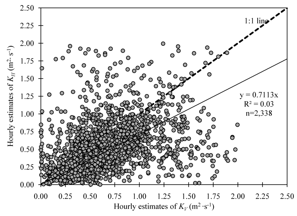
Figure 1.
Hourly estimates of KH against KV for growing and non-growing (dormant) seasons in 2005 and 2006 (pooled data).
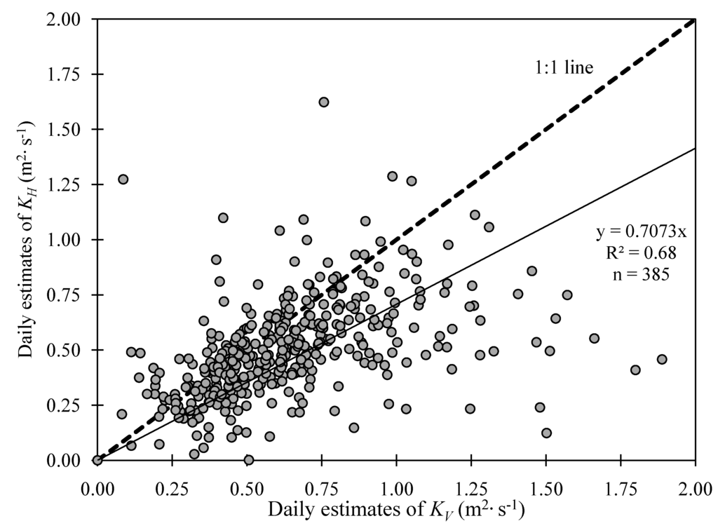
Figure 2.
Daily estimates of KH against KV for the growing and non-growing (dormant) seasons in 2005 and 2006 (pooled data).
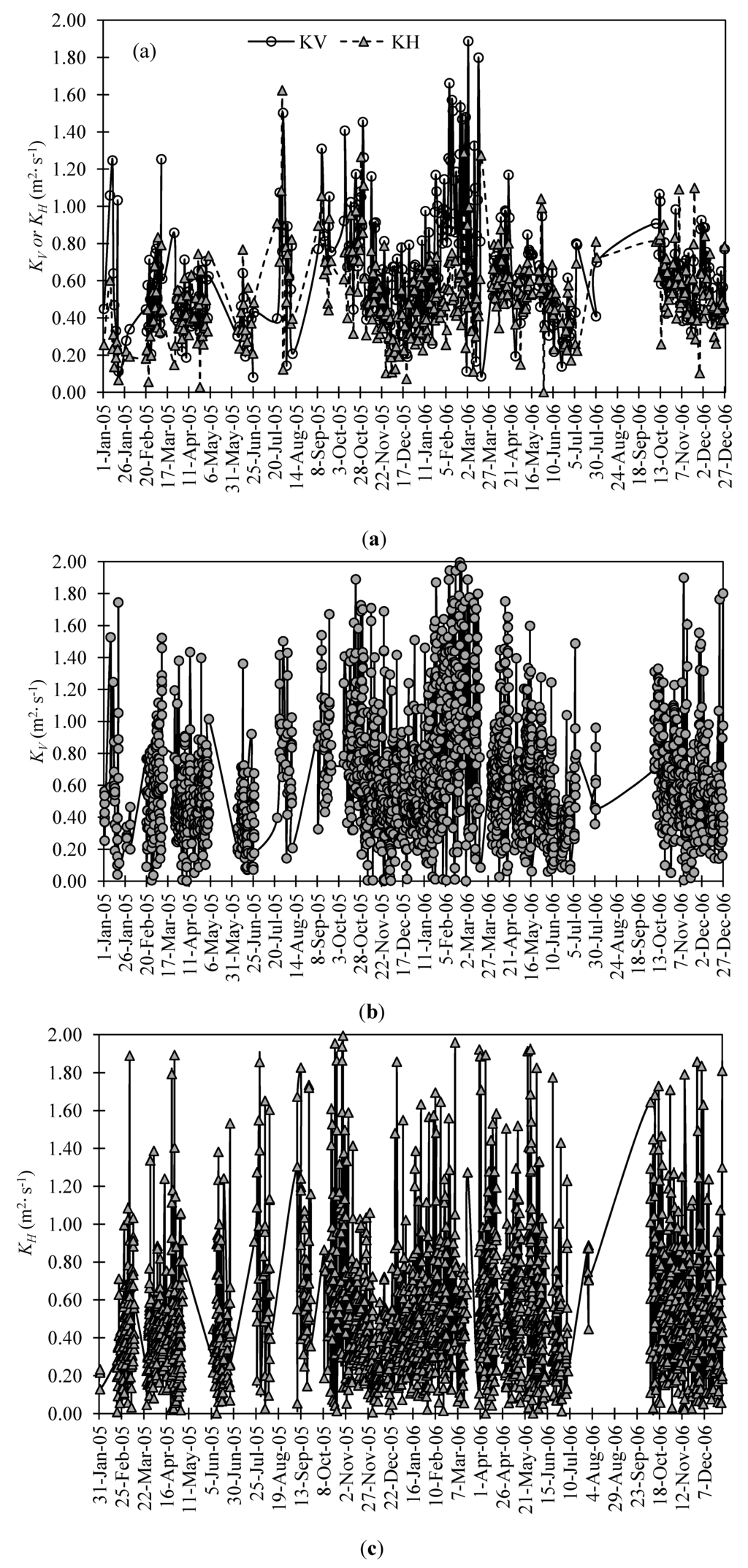
Figure 3.
(a) Seasonal variations of the daily estimates of KV and KH in 2005 and 2006 growing and non-growing (dormant) seasons; (b) Seasonal variations of the hourly estimates of KV; (c) Seasonal variations of the hourly estimates of KH.
Figure 3b,c represents distributions of hourly estimates of KV and KH, respectively, against time. In general, hourly estimates of KV ranges between approximately 0 m2∙s−1 to 1.8 m2∙s−1 and that of KH ranges approximately between 0 m2∙s−1 to 1.7 m2∙s−1. The higher and lower values of KV and KH appeared around the same times as those observed in Figure 3a. The seasonal distribution pattern that was discussed in the previous paragraph is quite clear in Figure 3b and Figure 3c. The first of the semiannual cycles begins around mid to late December and ends around late June. The second cycle begins promptly thereafter and ends around mid to late December. The numeric values for KV ranges from 0 m2∙s−1 to 0.9 m2∙s−1 during the troughs of the cycles and from 0 m2∙s−1 to 1.8 m2∙s−1 during crests of the cycles. The numeric values for KH approximately ranges from 0 m2∙s−1 to 0.7 m2∙s−1 during the troughs of the cycles and from 0 m2∙s−1 to 1.7 m2∙s−1 during crests of the cycles.
Figure 4 is the plot of the daily difference in KV and KH. The difference varied quite consistently during 2005 and 2006 seasons. During the earlier parts of the year (mid-January to late March) the difference remained quite high (approximately between 0.2 m2 s−1 to 1.2 m2 sec−1), which were lesser during late March to early May (approximately between −0.1 m2∙s−1 to 0.4 m2 sec−1). The difference remained quite low from early May to early October (approximately between −0.2 m2∙s−1 to 0.2 m2 ∙s−1). The difference was again slightly high during early October to early January of the following year (between −0.2 m2∙s−1 to 0.4 m2∙s−1). The study field was planted with maize during the both growing seasons in 2005 and 2006. Plants emerged around 12 May in 2005 and around 20 May in 2006, and were harvested on 17 October in 2005 and on 6 October in 2006. Combining this information along with the seasonal variations of the difference noticed in Figure 4, the difference between KV and KH tend to be higher during the non-growing (dormant) seasons than during the growing seasons. Moreover, it is also evident that during the dormant seasons the difference was lesser (approximately between −0.1 m2∙s−1 to 0.4 m2∙s−1) from early October to early January (of the following year) and again from late March to early May, and was greater (approximately between 0.2 m2∙s−1 to 1.4 m2∙s−1) from early to mid-January to late March.
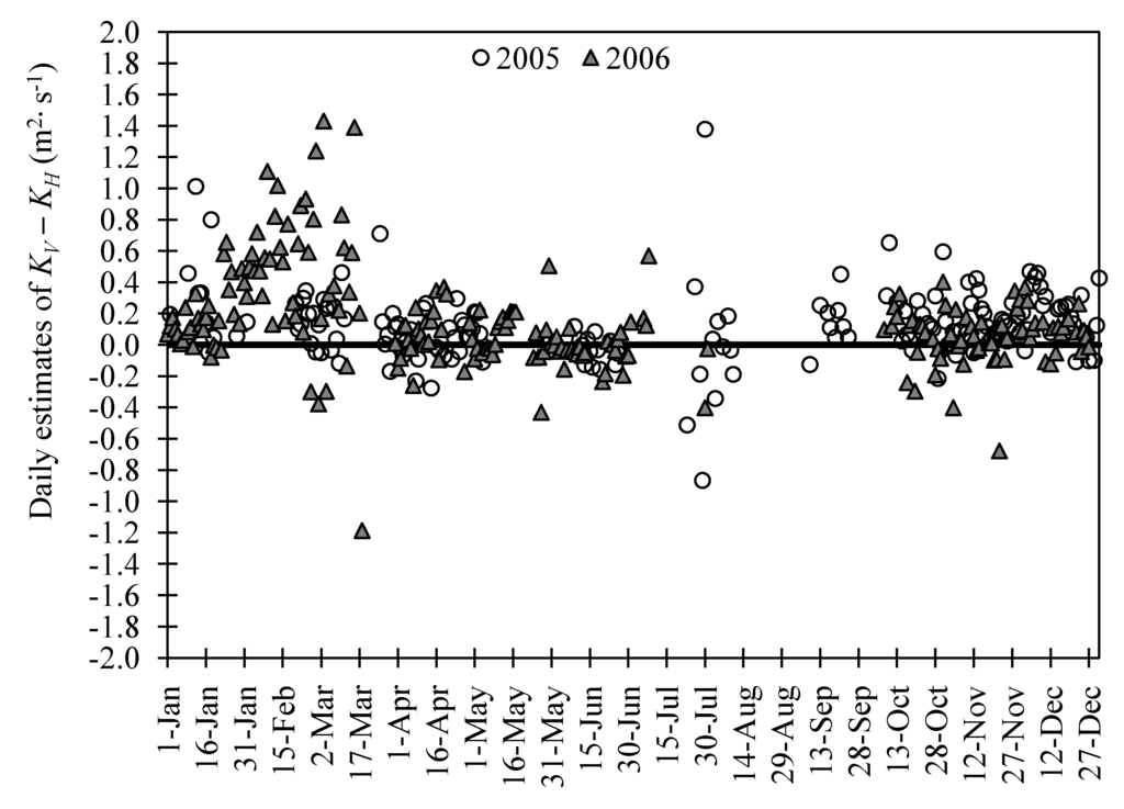
Figure 4.
Seasonal variations of daily estimates of KV – KH.
4.3. Diurnal Variations of KV and KH
For analyzing the diurnal variations in distribution patterns of KV and KH (Figure 5), the averages of KV and KH were calculated for every hour. KV ranges approximately between 0.2 m2∙s−1 and 0.8 m2∙s−1, and KH ranges approximately between 0.45 m2∙s−1 and 0.75 m2∙s−1. Except the fluctuation around 07:00, KV and KH stay very close to each other until about 10:00 in the morning, after which KH begins to decrease and reaches its lowest value around 17:00. KV, however, remains at its peak from about 10:00 to about 14:00 and then begins to decrease and reaches lowest value around 21:00. During the afternoon hours KV is generally higher than KH and during mornings and early evenings KH is higher than KV. Most interestingly, during the downfall KV follows a very similar downfall pattern as of KH, but with some time lag. These phenomena are probably the reasons why authors in [8] observed the difference between KV and KH to be higher during the afternoon.
The variation of the difference between KV and KH against time is presented in Figure 6. These differences were calculated by subtracting KH values from KV, both averaged for every hour. The difference is quite high (about 0.3 m2∙s−1) at 07:00 and then drops to a lower value (about −0.5 m2∙s−1) at 08:00. Then, it gradually increases with the hour and attains its maxima (of about 0.25 m2∙s−1) around 13:00, after which it gradually decays to the lowest value of about −0.3 m2∙s−1 in the evening.
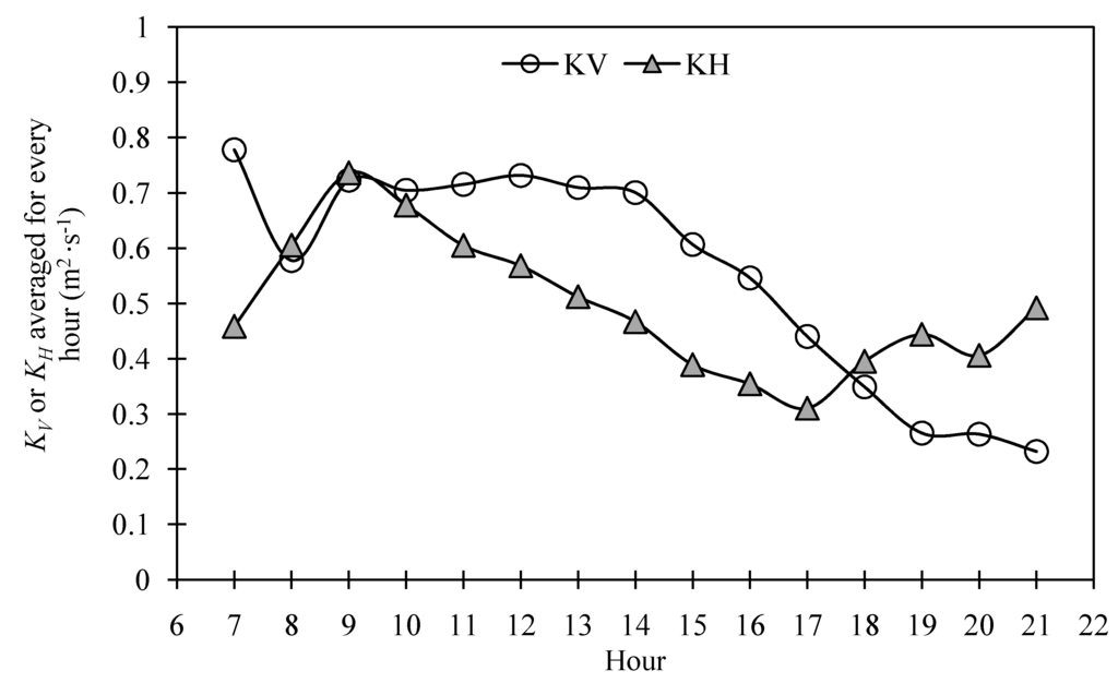
Figure 5.
Diurnal variations of KV and KH. The KV and KH in the Y-axis are the averages of KV and KH for every hour from 07:00 to 21:00 during the 2005 and 2006 growing and non-growing (dormant) seasons.
From Equation (1), it is evident that KV is the amount of latent heat flux rate at unit moisture gradient. Similarly, from Equation (2) it is evident that KH is the amount of sensible flux rate at unit temperature gradient. Therefore, higher values of KV or KH means a higher diffusion rates for latent or sensible heat, respectively. During very early morning hours the blackbody radiation by earthen materials (soil, canopy, etc.) exceeds the incoming energy, and this blackbody radiation acts as a source of energy. Since air is a gas, air reacts more promptly to this available energy in the form of blackbody radiation, which causes sensible heat diffusion. However, liquid water requires more energy to change phase, and as a result latent heat diffusion rate stays low during this time. This is why at 07:00, high value of KH and low value of KV was observed. During the latter part of the morning, the incoming solar radiation warms up atmospheric gases and liquid water. This increases the internal energy of the atmospheric gases, a process that tends to shift the whole environment from colder to warmer condition. During this period, a large fraction of incoming solar radiation is used to warm up the environment and, therefore, only a smaller fraction is available for diffusion of heat. As a result, during early morning both KV and KH are low and both gradually increase with time. However, once the liquid water and atmospheric gases reach equilibrium with the incoming solar radiation, any further heating primarily increases the atmospheric air temperature more quickly. During this time, it is assumed that warmer air could radiate enough energy that can act as the secondary source of energy for latent heat diffusion and, thereby, the atmospheric gases release some of its additional heat and evaporate more water. These phenomena cause sensible heat diffusion rate (KH) to decrease from its peak, but the latent heat diffusion rate (KV) retains its peak rate for little longer. During the afternoon, amount of incoming solar radiation begins to decrease, which initiates the cooling down of the environment. Therefore, after about 14:00 KV also starts decreasing from its peak. Similar phenomenon was reported by [30], showing a slower evaporation rates from lakes during the earlier part of the year (colder to warmer) than during the latter part of the year (warmer to colder).
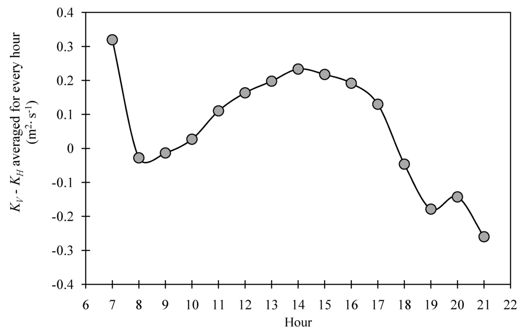
Figure 6.
Average of the diurnal variations of KV – KH estimated for every hour from 07:00 to 21:00. The KV – KH in the Y-axis are the averages of KV – KH for every hour during the 2005 and 2006 growing and non-growing (dormant) seasons.
4.4. Correction for Inequalities between KV and KH
4.4.1. Theoretical Analysis for Correction of KV and KH
From the above discussion it is quite evident that KV is not equal to KH for the most of the times, even during the micrometeorological conditions in which they should be theoretically equal. Therefore, any estimation made based on the equality assumption may introduce some errors in the final latent and sensible heat values. Previous researchers proposed different procedures for developing a correction factor for the inequality. However, these procedures require additional micrometeorological information/measurements that are not readily available from all Bowen ratio systems, making the procedures difficult to apply in practice. In the following section developing correction terms using micrometeorological parameters that are easily measured or estimated by any Bowen ratio system was attempted.
Authors in [15] investigated the behaviors of the ratio KH to KV in terms of two new diffusion coefficients Kα and Kd, they defined as the diffusivity for the “total convective heat flux” and the diffusivity for the difference between “sensible and latent heat flux,” respectively. Following the same concept, the equations for Kα and Kd, respectively, can be rewritten as:
and
where (∂φ/∂z) and (∂θ/∂z) can be defined as:
Therefore, it can be shown from Equations (1), (2), (12), and (13) that KV and KH can be estimated in terms of
and
as:
Both (
) and (
) behave differently during the morning hours (until solar noon) than during the afternoon hours. Distribution of (
) against (∂φ/∂z + ∂θ/∂z), averaged for every hour is presented in Figure 7a and distribution of (
) against (∂φ/∂z − ∂θ/∂z), averaged for every hour is presented in Figure 7b. When plotted against (∂φ/∂z + ∂θ/∂z), (
) takes different path (higher slopes) while increasing from a lower value during morning hours, than while decreasing (lower slopes) from the peak during afternoon hours. Also, when plotted against (∂φ/∂z − ∂θ/∂z), (
) follows similar, but opposite patterns. The term (
) begins from highest value during the earliest part of the day, and decreases with time during the day. The term (
) takes lower slope while decreasing from its highest value during morning hours, and takes higher slopes while increasing from the lowest value during afternoon hours. Therefore, both (
) and (
) have one very similar property that their forward and reverse paths are different (Figure 7a,b). These phenomena are very similar to a “hysteresis loop”, which indicates different forward and backward paths and the area in between, which represents loss of energy.
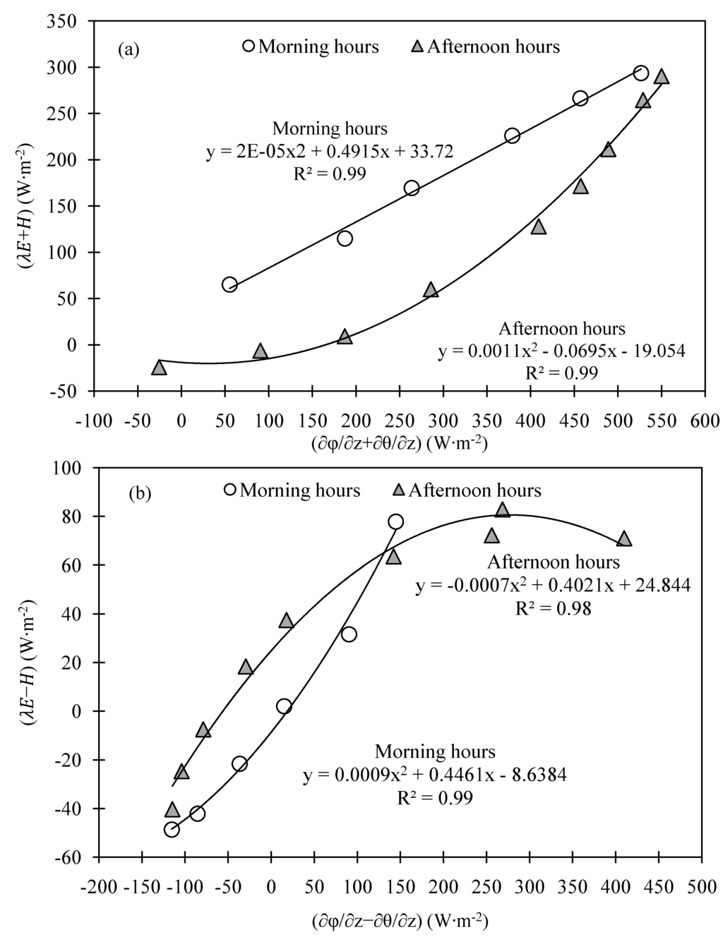
Figure 7.
(a) Latent heat plus sensible heat (𝜆𝐸 + 𝐻) vs. moisture gradient and sensible heat gradient (∂φ/∂z + ∂θ/∂z); (b) Expression of the difference between latent and sensible heat (λE − H) as a function of the difference between moisture gradient and sensible heat gradient (∂φ/∂z − ∂θ/∂z).
Both sensible and latent heat fluxes are extremely dynamic and seasonal variables. Therefore, it is quite obvious that the maxima and minima, and probably the slopes of the best fit curves observed in Figure 7a,b may also vary seasonally. The total available energy for the surface (Rn − G) is also a seasonal variable. Therefore, the total available energy as a “proxy” can be used for a variable representing the seasonal variations. Three dimensional distributions of (
) against (∂φ/∂z + ∂θ/∂z) and (Rn − G) and 3D distributions of (
) against (∂φ/∂z − ∂θ/∂z) and (Rn − G) were presented in Figure 8a,b, respectively. The straight lines passing through the origin (0, 0, 0) show the locations of the origins. From both Figure 8a and Figure 8b, both (
) and (
) are linearly correlated with (Rn − G). When (Rn − G) increases, (
) increases as well; again when (Rn − G) increases, (
) decreases. The quadratic nature of the relationships between (
) and (∂φ/∂z + ∂θ/∂z), and (
) and (∂φ/∂z − ∂θ/∂z) were already established in Figure 7b. Therefore, combining the information obtained from Figure 7a,b, and Figure 8a, b; (
) can be estimated as:
where, a0, a1, and a2 are regression parameters. The numeric values of a0, a1, and a2 are expected to be different during morning hours than during the afternoon hours. Similarly, (
) can be empirically estimated as:
with different numeric values for the regression parameters b0, b1, and b2 during the morning hours than during the afternoon hours.
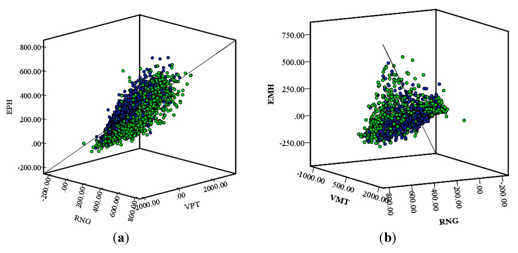
Figure 8.
(a) 3D plot of (𝜆𝐸+𝐻; W m−2) (presented as EPH) against (∂φ/∂z + ∂θ/∂z; W∙m−2) (presented as VPT) and total available energy (presented as RNG). The darker color represent morning hours and the lighter color represent the afternoon hours; (b) 3D plot (𝜆𝐸 − 𝐻; W∙m−2) (presented as EMH) against (∂φ/∂z − ∂θ/∂z; W∙m−2) (presented as VMT) and total available energy (presented as RNG). The darker color represent morning hours and the lighter color represent the afternoon hours.
4.4.2. Empirical Estimation of Bowen Ratio
From Equations (6) and (7) it is evident that any error caused by the inequality between KH to KV would impact estimation of Bowen ratio. The estimated Bowen ratio then impact latent heat and sensible heat estimations. For the same reason, any correction factor for the inequality between KH to KV would impact the Bowen ratio estimation, which in turn would rectify the latent and sensible heat estimations. Therefore, in this research, instead of investigating the behaviors of Kα and Kd and, thereby, estimating the ratio of KH to KV, the behavior of (λE + H) was investigated mainly as a function of (∂φ/∂z + ∂θ/∂z) and (Rn − G) and behavior of (λE – H) mainly as a function of (∂φ/∂z − ∂θ/∂z) and (Rn − G). It is noted that Kα is a partial derivative of λE + H with respect to (∂φ/∂z + ∂θ/∂z) and Kd is the partial derivative of (λE – H) with respect to (∂φ/∂z − ∂θ/∂z).
In the following section, a demonstration was shown as to how rectification for inequalities between KV and KH may be implemented. The quadratic nature of relationships between (λE + H), and (Rn – G) and (∂φ/∂z + ∂θ/∂z) for morning and afternoon hours was tested by selecting different segments from the dataset, and the nature of data distributions, presented in Equations (18) and (19), are valid in all those segments. Therefore, Equations (18) and (19) were used to empirically estimate λE + H and λE − H, respectively. The eddy covariance hourly latent and sensible heat data were used to calculate the response variables and regression parameters were estimated using nonlinear fit, separately for morning hours and for afternoon hours. All the iterations, for the nonlinear regression models, converged. The final regression equations were:
Once λE + H and λE − H were empirically estimated they were solved for λE and H and were used to estimate the “corrected Bowen ratio”. Therefore, the corrected Bowen ratio equation can be written as:
where, λE and H were estimated by solving Equations (20) and (21). Finally, the estimated βr was used to estimate
and H as:
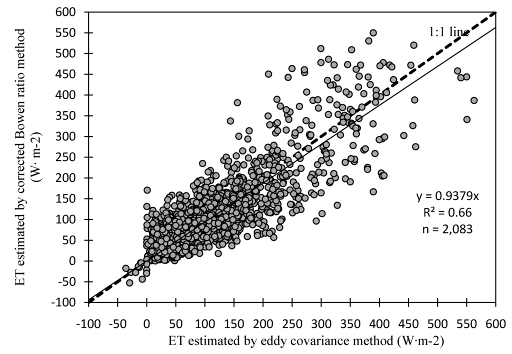
Figure 9.
Comparisons between corrected hourly Bowen ratio ET estimation against eddy covariance hourly ET data for the growing and non-growing (dormant) seasons in 2005 and 2006.
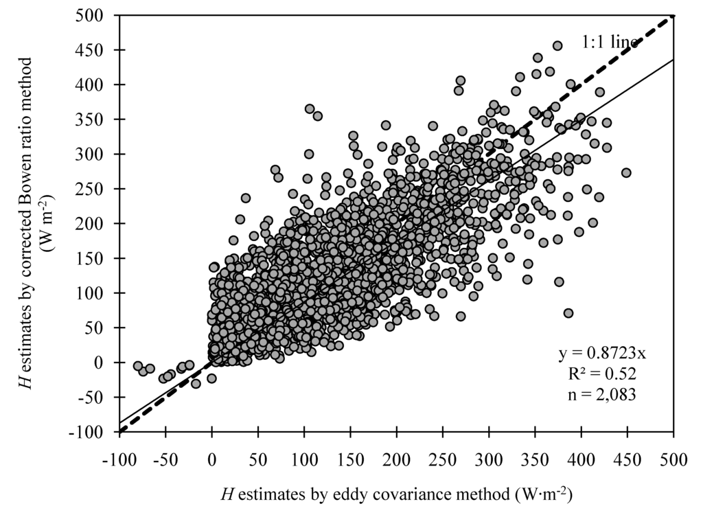
Figure 10.
Comparisons of hourly estimations of corrected Bowen ratio H against the eddy covariance H data for growing and non-growing (dormant) seasons in 2005and 2006.
The author in [29] pointed out two scenarios when Bowen ratio estimations cannot be reliable: (i) if βr in Equation (23) approaches negative unity, the denominator approaches zero, and as a result the latent or sensible heat estimations becomes unreasonably large; (ii) the second phenomenon in known as counter gradient phenomenon. From Equation (1) it is evident that a negative upward vapor pressure gradient should cause a positive upward diffusion flux. The opposite is also true for the positive downward flux. However, during counter gradient phenomenon this simple law fails, and as a result, positive upward flux estimation can be noticed even during a positive upward vapor pressure gradient. During such scenarios, the Bowen ratio ET estimation can be erroneous. Therefore, all incidents showing counter gradient phenomena and all the incidents when 0.75 > βr > −1.25 were disregarded to avoid such situations.
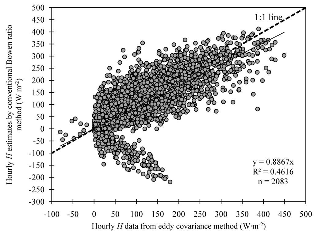
Figure 11.
Comparisons between conventional Bowen ratio H estimates against eddy covariance H estimates for the growing and non-growing (dormant) seasons in 2005 and 2006.
Distribution of hourly corrected Bowen ratio ET estimations against hourly eddy covariance ET data are presented in Figure 9. The slope of the best fit line passing through the origin is 0.9379. Apparently, the adjustment for the inequalities between KV and KH have changed very little in Bowen ratio ET estimation, as the slope of the best fit line passing through the origin changed only from 0.9201 to 0.9379 (the plot of eddy covariance ET against conventional Bowen ratio ET are not shown). Similar results have also been reported by [6,7]. Similarly, the distribution of corrected hourly Bowen ratio H estimation against hourly eddy covariance H data are presented in Figure 10. The slope of the best fit line passing through the origin is 0.8723. Even though adjustments for KV and KH have changed very little in Bowen ratio ET estimation, this adjustment has considerably influenced Bowen ratio H estimation. In Figure 11, the conventional Bowen ratio H estimation against the eddy covariance H data were compared. There were considerable number of hours during which Bowen ratio H estimation were opposite in signs as compared with the eddy covariance H data. During these hours, even though eddy covariance estimated positive H conventional Bowen ratio estimated negative H. These results indicate that the adjustments (rectification) for the inequalities between eddy diffusivities is quite essential at least for sensible heat estimation, and may be important for application of the Bowen ratio method for estimation of diffusion fluxes of other gases.
5. Conclusions
The main focus of this research was to test the assumption of equality between KV and KH and their impact on latent and sensible heat flux estimations by the Bowen ratio method, to further investigate the potential causes of inequalities for a non-stressed subsurface drip-irrigated maize canopy, and to investigate a rectification procedure for the inequalities using micrometeorological variables. Both diurnal and seasonal variations of KV and KH were investigated. Although both KV and KH varied seasonally, seasonal variations have little impact on their differences. The diurnal variations were the most influential on the distributions of KV and KH and their differences. Thus, perhaps the most promising approach for rectifying for the inequalities between on the distributions of KV and KH is to study the slope of
with respect to (∂φ/∂z + ∂θ/∂z) and the slope of
with respect t
, and to estimate the corrected Bowen ratio using the calculated
and
. However, the study has enlighten an important characteristic of the latent and sensible heat diffusivities- KV is less than KH during morning hours (until noon), and is greater than KH during afternoon hours (afternoon). Since diffusivity (KV or KH) represents the diffusion rate per unit gradient, it is suggested that during the earlier part of the day when the atmosphere is approaching from a colder to warmer environment the sensible heat diffusion rate and latent heat diffusion rates are very close to each other. However, during the latter part of the day (mainly during the afternoon) the latent heat diffusion rate is higher than the sensible heat diffusion rate.
The most important outcome of the analysis on diurnal variations of KV and KH is that, during very early morning hours, blackbody radiations from earthen materials (soil, plant canopy, etc.) acts as a secondary source of energy. This energy is primarily used in sensible heat diffusion, causing KH to be high. Also, the sensible heat contained within the atmospheric gases behaves as the secondary source of energy for latent heat diffusion, during the afternoon hours. During the afternoon, when the atmosphere is already warm enough and reaches equilibrium with the incoming solar radiation, the warm atmosphere supplies additional energy for further diffusion of latent heat. This is why it was observed that, even though during morning hours, latent heat diffusion rate and sensible heat diffusion rate are very close to each other, during afternoon hours latent heat diffusion rate is considerably higher than the sensible heat diffusion rate. The latent heat diffusion rate remains at its peak for a few hours and then begins to descend, following a very similar slope as of the sensible heat diffusion rate. However, latent heat diffusion rate still remain higher than sensible heat diffusion rate until sometime in the early evening.
One of the most promising approach for rectifying for the inequalities between on the distributions of KV and KH is to study the slope of
with respect to (∂φ/∂z + ∂θ/∂z) and the slope of
with respect t
, and to estimate the corrected Bowen ratio using the calculated
and
. The rectification for KV or KH had a little impact on the Bowen ratio latent heat flux estimation; however, it had considerable impact on the Bowen ratio sensible heat flux estimation. Therefore, it is suggested that this type of rectifications is quite important for Bowen ratio estimations and may potentially be useful for application of Bowen ratio method for estimating other gases (i.e., CO2) as well. Further research is needed to assess the performance of the rectification procedures developed for estimation of the other fluxes for other vegetation surfaces.
Author Contributions
All authors have contributed to the idea and hypothesis development, method development, analyses, interpretation of the results and writing the manuscript.
Conflicts of Interest
The authors declare no conflicts of interest.
Disclaimer
The mention of trade names or commercial products is for the information of the reader and does not constitute an endorsement or recommendation for use by the University of Nebraska-Lincoln or the authors.
References
- Alfieri, J.G.; Blanken, P.D.; Smith, D.; Morgan, J. Concerning the measurement and magnitude of heat, water vapor,and carbon dioxide exchange from a semiarid grassland. J. Appl. Meteorol. Clim. 2009, 48, 982–996. [Google Scholar] [CrossRef]
- Bowen, I.S. The ratio of heat losses by conduction and by evaporation from any water surface. Phys. Rev. 1926, 27, 779–787. [Google Scholar] [CrossRef]
- Monin, A.S.; Obukhov, A.M. The basic laws of turbulent mixing in the surface layer of the atmosphere. Akad. Nauk. SSSR Trud. Geofiz. Inst. 1954, 24, 163–187. [Google Scholar]
- Gavilan, P.; Berengena, J. Accuracy of the Bowen ratio-energy balance method for measuring latent heat flux in a semiarid advective environment. Irrig. Sci. 2007, 25, 127–140. [Google Scholar] [CrossRef]
- Brotzge, J.A.; Crawford, K.C. Examination of the surface energy budget: A comparison of Eddy correlation and Bowen ratio measurement systems. J. Hydrometeorol. 2003, 4, 160–178. [Google Scholar] [CrossRef]
- Lee, X.H.; Yu, Q.; Sun, X.M.; Liu, J.D.; Min, Q.W.; Liu, Y.F.; Zhang, X.Z. Micrometeorological fluxes under the influence of regional and local advection: A revisit. Agric. For. Meteorol. 2004, 122, 111–124. [Google Scholar] [CrossRef]
- Laubach, J.; McNaughton, K.G.; Wilson, J.D. Heat and water vapor diffusivities near the base of a disturbed internal boundary layer. Bound. Layer Meteorol. 2000, 94, 23–63. [Google Scholar] [CrossRef]
- De Bruin, H.A.R.; van den Hurk, B.J.J.M.; Kroon, L.J.M. On the temperature-humidity correlation and similarity. Bound. Layer Meteorol. 1999, 93, 453–468. [Google Scholar]
- Lang, A.R.G.; McNaugton, K.G.; Fazu, C.; Bradley, E.F.; Ohtaki, E. Inequality of eddy transfer coefficients for vertical transport of sensible and latent heats during advective inversions. Bound. Layer Meteorol. 1983, 25, 25–41. [Google Scholar] [CrossRef]
- Motha, R.P.; Verma, S.B.; Rosenberg, N.J. Exchange of coefficients under sensible heat advection determined by eddy correlation. Agric. For. Meteorol. 1979, 20, 273–280. [Google Scholar] [CrossRef]
- Verma, S.B.; Rosenberg, N.J.; Blad, B.L. Turbulent exchange coefficients for sensible heat and water vapor under advective conditions. J. Appl. Meteorol. 1978, 17, 330–338. [Google Scholar] [CrossRef]
- Warhaft, Z. Heat and moisture flux in the stratified boundary layer. Q. R. J. Meterol. Soc. 1976, 102, 703–720. [Google Scholar] [CrossRef]
- Blad, B.L.; Rosenberg, N.J. Lysimetric calibration of the Bopwen ratio-energy balance method for evapotranspiration estimation in the Central Great Plains. J. Appl. Meteoreol. 1974, 13, 227–236. [Google Scholar] [CrossRef]
- Laubach, J.; Raschendorfer, M.; Kreilein, H. Determination of heat and water vapour fluxes above a spurse forest by eddy correlation. Agric. For. Meteorol. 1994, 71, 373–401. [Google Scholar] [CrossRef]
- McNaughton, K.G.; Laubach, J. Unsteadiness as a cause of non-equality of eddy diffusivities for heat and vapour at the base of an advective inversion. Bound. Layer Meteorol. 1998, 88, 479–504. [Google Scholar] [CrossRef]
- Irmak, S.; Mutiibwa, D. On the dynamics of stomatal resistance: Relationships between stomatal behavior and micrometeorological variables and performance of Jarvis-type parameterization. Trans. ASABE 2009, 52, 1923–1939. [Google Scholar] [CrossRef]
- Priestley, H.B.; Swinbank, W.C. Vertical transport of heat by turbulence in the atmosphere. Proc. R. Soc. Lond. Ser. A Math. Phys. Sci. 1947, 189, 543–561. [Google Scholar] [CrossRef]
- Swinbank, W.C. The measurement of vertical transfer of heat and water vapor by eddies in the lower atmosphere. J. Meteorol. 1951, 8, 135–145. [Google Scholar] [CrossRef]
- Irmak, A.; Irmak, S. Reference and crop evapotranspiration in South Central Nebraska. II: Measurement and estimation of actual evapotranspiration for corn. J. Irrig. Drain. Eng. 2008, 134, 700–715. [Google Scholar]
- Irmak, S.; Mutiibwa, D. On the dynamics of evaporative losses from Penman-Monteith with fixed and variable canopy. Trans. ASABE 2009, 52, 1139–1153. [Google Scholar] [CrossRef]
- Irmak, S. Nebraska water and energy flux measurement, modeling, and research network (NEBFLUX). Trans. ASABE 2010, 53, 1097–1115. [Google Scholar] [CrossRef]
- Irmak, S.; Mutiibwa, D. On the dynamics of canopy resistance: Generalized-linear estimation and its relationships with primary micrometeorological variables. Water Resour. Res. 2010, 46, 1–20. [Google Scholar] [CrossRef]
- Finnigan, J.J.; Clement, R.; Malhi, Y.; Leuning, V.; Cleugh, H.A. A re-evaluaion of long-term flux measuremtn techniques Part I: Averaging and coordinate rotation. Bound. Layer Meteorol. 2003, 107, 1–48. [Google Scholar] [CrossRef]
- Schotanus, P.; Neuwstadt, F.T.M.; de Bruin, H.A.R. Temperature measurement with a sonic anemometer and its application to heat and moisture fluxes. Bound. Layer Meteorol. 1983, 26, 81–93. [Google Scholar] [CrossRef]
- Kaimal, J.C.; Businger, J.A. A continuous wave sonic anemometer-thermometer. J. Appl. Meteorol. 1963, 2, 156–164. [Google Scholar] [CrossRef]
- Van Dijk, A.; Kosher, W.; de Bruin, H.A.R. Oxygen sensitivity of Krypton and Lyman-α hygrometers. J. Atmos. Ocean. Technol. 2003, 20, 143–151. [Google Scholar]
- Moore, C.J. Frequency response corrections for eddy correlation systems. Bound. Layer Meteorol. 1986, 37, 17–35. [Google Scholar] [CrossRef]
- Webb, E.K.; Pearman, G.I.; Leuning, R. Correction of flux measurements for density effects due to heat and water vapour transfer. Q. R. J. Meteorol. Soc. 1980, 106, 85–100. [Google Scholar] [CrossRef]
- Ohmura, A. Objective criteria for rejecting data for Bowen-Ratio flux calculations. J. Appl. Meteorol. 1982, 21, 595–598. [Google Scholar] [CrossRef]
- Veihemeyer, F.J. Evapotranspiration. In Handbook of Applied Hydrology; Chow, V.T., Ed.; McGraw-Hill Company: New York, NY, USA, 1964; pp. 11:1–11:38. [Google Scholar]
© 2014 by the authors; licensee MDPI, Basel, Switzerland. This article is an open access article distributed under the terms and conditions of the Creative Commons Attribution license (http://creativecommons.org/licenses/by/3.0/).