Abstract
This study extends prior research on referee bias and close bias in professional soccer by examining whether Major League Soccer (MLS) referees’ discretion over stoppage time (i.e., extra play beyond regulation) is influenced by end-of-regulation match scores and/or home field advantage. To do so, we employ a grouped-data regression model and a partially adaptive model. Both account for the imprecise measurement in reported stoppage time. For the 2011 season we find no home field advantage. In fact, stoppage time is the same with a one or two goal deficit at the end of regulation, regardless of which team is ahead. However, the 2011 results do point to an increase in stoppage time of 12 to 20 seconds for nationally televised matches. For the 2012 season, the nationally televised effect disappears due to an increase in stoppage time for those matches not nationally televised. However, a home field advantage is present. Facing a one-goal deficit at the end of regulation, the home team receives about 33 seconds more stoppage time than a visiting team facing the same deficit.
JEL codes:
L8; L83; L2; C20
1. Introduction
There is evidence of a home field advantage in many sports over many years in studies too numerous to mention. Recently, however, the existence of a home field advantage has been challenged. In their book, Scorecasting, after listing all of the usual explanations for the existence of a home field advantage, Moskowitz and Wertheim [1] settle on the impact of fans on officiating—what is called referee bias. Referee bias is of great interest in soccer. Soccer referees have enormous discretion which extends to the determination of the amount of extra time added to regulation time, thereby increasing the length of the match. Given the typically low scoring in soccer, the officials have a greater likelihood of making decisive calls. Consider a comparison to professional football in the U.S.—the National Football League (NFL). As in soccer, each football team has eleven players, there is a smaller playing field, there are seven officials with different monitoring responsibilities, and important referee decisions are automatically reviewed by the Replay Booth, which uses instant replay to look for evidence of an incorrect ruling made during play, in which case the ruling is overturned. In addition, coaches can challenge some referee decisions and request that the decision on the field be reviewed by the Replay Booth. In comparison, however, a soccer referee has considerably more responsibility and discretion, given that he/she also has the authority to lengthen regulation playing time.
Many empirical studies have examined whether this discretion is used to favor the home team. Generally speaking, these studies use least squares regression models, wherein stoppage time at the end of the match is included as the dependent variable. Independent variables include the score at the end of regulation, the number of second half yellow cards, the number of second half red cards, and the number of second half substitutions. Other independent variables frequently used in these models are match attendance, stadium capacity, venue fixed effects, referee fixed effects, whether the stadium has a track around the field, effectively keeping spectators at a distance. For example, Sutter and Kocher [2] examine penalties and the awarding of extra time at the end of matches in the 2000–2001 season of the German Bundesliga and find evidence of a home bias. Scoppa [3] examines stoppage time in Italian soccer league Serie A and finds that referees are biased in favor of the home team by adding more stoppage time if the home team is losing. They also find that the bias is larger if there is no running track in the stadium.
Garicano, Palacios-Huerta, and Prendergast [4] investigate the role that social forces may have on the behavior of individuals. Specifically, they offer an empirical test to analyze deviations from honest behavior in a sports context by addressing how the preferences of the crowd attending a soccer match affect referee behavior. Using data from the Primera División in Spain that includes the score difference, number of yellow and red cards, substitutions, and stoppage time added to the end of each match for the 1994–1995 and 1998–1999 seasons, they conduct a regression to test for systematic bias in favor of home teams based on stoppage time added. Their results show that professional soccer referees systematically favor home teams by shortening close matches when the home team is ahead, and lengthening close matches when the home team is behind. Garicano et al. [4] further document how the size and the composition of the crowd affect referee favoritism, and conclude that referees favor home teams in order to satisfy crowds in the stadium. Dawson and Dobson [5] examine international matches and find that social pressure, such as that found in [4], is important, as are the nationality of the referee and the club and the reputation of the league. Rickman and Witt [6] look at the impact of the change to professional referees on outcomes in English soccer and find, however, that after the change, the home field advantage, as measured by stoppage time, disappeared. Dohmen [7], using data from twelve Bundesliga seasons, finds that referees systematically award more stoppage time in close matches when the home team is behind and that the home field advantage is stronger in stadiums without a running track. He also finds evidence that referees favor the home team in awarding goals and penalty kicks. Pettersen-Lidbom and Priks [8] examined an unusual episode in Italian soccer to search for referee bias. In 2007, after several riots, some teams were forced to play matches in empty stadiums. This resulted in a unique situation where some matches had fans present and others did not, providing an opportunity to determine whether the fans were influencing the referees. Using data from the 2006–2007 season for Serie A and Serie B matches, the authors find, using least squares regression, evidence of referee bias.
Recently, studies have examined the issue of referee bias using minute-by-minute data on match activity. Using this detailed data for English and German soccer matches, Buraimo, Forrest, and Simmons [9] examine the occurrence of yellow cards and reds cards and find evidence of pure referee bias. They also find that in Germany home teams with running tracks receive more yellow and red cards. Using similarly detailed data, Buraimo, Simmons, and Maciaszczyk [10] examine the probability of awarding yellow cards in Spain’s La Liga and UEFA Champion’s League and find evidence of a home team bias.
A new line of research is investigating other motivations for referee bias. For example, in an important paper on referee bias, Price, Remers, and Stone [11] examine profit-maximizing biases of referees in the National Basketball Association (NBA). They find that referees are likely to favor home teams, teams losing during games, and teams losing in playoff series. These last two biases are referred to as close bias. These authors explain how home bias causes games to be more enjoyable and may lead fans to think their attendance matters, thus increasing ticket demand, while close bias would increase television viewership demand and possibly ticket demand as well.
One manifestation of close bias in soccer may be an increase in stoppage time if a match is televised. In light of the growing importance of television revenue, this issue deserves scrutiny. As sports change from gate-driven revenues to television-driven (or media-driven) revenues, the relative importance of home bias and close bias should change as well, with close bias becoming more important. This study examines home bias and close bias using data from the 2011 and 2012 Major League Soccer (MLS) seasons. We seek to explain added time at the end of the match as a function of the usual independent variables: score at the end of the match, number of second half yellow cards, number of second half red cards, number of second half substitutions and team and referee fixed effects. There are, however, several novel features of our study. We use data from the two most recent MLS seasons, 2011 and 2012, and we include a dummy variable to investigate the existence of a television effect on stoppage time. We also note that reported stoppage time is interval-censored and consequently, instead of using ordinary least squares, we estimate a grouped-data regression model. Further, in order to relax the distributional assumption of normality in the grouped-data regression model, we estimate a partially adaptive regression model following Caudill and Long [12].
Our findings indicate that there is no home field advantage in the awarding of stoppage time in 2011. The most stoppage time is added to a match that is tied at the end of regulation, and we find only about 12 seconds less stoppage time is added if there is a one or two goal difference, regardless of which team is behind. We do find a positive television effect on stoppage time. In particular, about 12 seconds more stoppage time is added for a nationally televised match, ceteris paribus. Our results for 2012 more closely resemble previous work on stoppage time. We do find evidence of a home field advantage. In particular, if the home team is behind by one goal at the end of regulation, about 26 seconds more stoppage time is added beyond what a visiting team facing a one-goal deficit would receive. We find no evidence of a television bias in 2012. One possible explanation for the reversal, certainly as far as the impact of television is concerned, is that MLS’ contract with FOX expired in 2011, and MLS was in the process of courting FOX’s rival NBC. Longer matches might translate into more MLS viewers and a more lucrative television contract from MLS’s perspective.
2. Stoppage Time and Television Rights in MLS: An Overview
Due to the important roles played by the measurement of stoppage time and MLS television rights in our analysis, this section provides an overview of each.
2.1. Stoppage Time in Soccer
Soccer differs from many team sports in that its 90-minute play clock is not stopped during play, except for half-time or intermission. This feature, in combination with the fact that after the 90 minutes of regulation play, soccer referees have discretion over allowing or disallowing additional time for play—a concept that is officially known as “allowance for time lost”—provides what is arguably the greatest distinction between soccer and its professional sports counterparts of American football, basketball and others. Rules regarding the duration of soccer matches, and in particular what constitutes allowance for time lost, are covered in “Law 7” of the Fédération Internationale de Football Association’s (FIFA) official Laws of the Game. Allowances provided for by FIFA include compensating for administrative stoppages or player substitutions, disciplinary warnings or bookings, and/or treatment of injuries. FIFA’s Laws also confirm that “... the allowance for time lost is at the discretion of the referee ([13], p.28).” Later in the Laws, the procedure for allowance for time lost is clarified:
The fourth official indicates the minimum additional time decided by the referee at the end of the final minute of each period of play. The announcement of the additional time does not indicate the exact amount of time left in the match. The time may be increased if the referee considers it appropriate but never reduced (FIFA, 2011: 98).
Again, the referee has sole discretion in decisions regarding stoppage time.
2.2. MLS and Television
ESPN has been covering MLS matches since the league’s debut in 1995. The network partnered with ABC on a three-year deal with MLS, wherein ESPN and ESPN2 would televise 35 matches and ABC would broadcast the MLS Cup. According to the agreement, ESPN would not pay rights fees, although the two entities would share advertising revenues [14]. By 2006, MLS had reached a new eight-year agreement with ESPN and ABC that was reportedly worth between $7 million and $8 million per year [15,16]. According to the new agreement, ESPN2 would televise 26 regular season matches in prime time (Thursdays), in addition to three playoff contests, while ABC would broadcast each season’s opening match, the all-star match, and the MLS Cup. The deal also included television coverage of the first round of the MLS Draft, and spanned many of the network’s associated media—ESPN, ESPN2, ESPN360, Mobile ESPN and ESPN Deportes [16].
After the first two years of the new agreement, ESPN’s affiliates subsumed the coverage provided previously by ABC, and ESPN2 terminated its Thursday night schedule in favor of a “game of the week” format designed to reverse low ratings from the first two years of the new contract [17]. In making the move, ESPN cited more flexibility in offering live lead-in coverage of matches under the new format, and an increased opportunity to feature the league’s marquee teams. These changes were made to address a decline in viewership, which fell from an average of 289,000 viewers per match in 2007, to 253,000 viewers per match in 2008 [17].
MLS also had a contract with Fox Soccer beginning in 2003. Additionally, in August of 2011, the NBC network entered the arena when MLS and NBC Sports agreed to a three-year deal to televise 45 league matches and four United States national team matches across NBC and NBC Sports Network. This deal ended MLS’ near decade long partnership with FOX Soccer, which fulfilled a one-year contract for 2011 [15,18]. In making the switch, MLS lauded the fact that the NBC Sports Network reached 76 million homes, compared to the 39 million homes reached by FOX Soccer [15]. Also underlying the switch was the widely-held view of MLS that, throughout the partnership, FOX was primarily focused on the English Premier League and, thus, did little to promote MLS [18].
For a reported $10 million per year, NBC had purchased rights to broadcast two regular-season MLS matches, two playoff matches and two national team matches, while the NBC Sports Network was set to televise 38 regular-season matches, three playoff matches and two national team matches [18]. MLS believes its partnership with NBC is a good one, given what Spanberg [19] refers to as “... NBC’s blend of strong storytelling and combination of 20 TV networks and 40 digital networks can give the sport cachet and exposure few can match.” According to [19], even with the new MLS-NBC deal, ESPN will, through the 2014 season, air 21 regular-season matches split among ESPN, ESPN2 and ESPN Deportes, as well as the all-star game and MLS Cup, with Univision holding Spanish-language rights. In promoting itself to MLS, NBC cited a number of positive trends, including a building boom in soccer-specific stadiums, several of which maintain unsold naming rights, and a 7.2 percent increase in soccer attendance in 2011 [19].
3. The Data and Model
The data used in this study come from the MLS website, and include information on each regular season match during the 2011 and 2012 MLS seasons. There are currently 18 teams in MLS, and each plays 34 matches per season, with 17 of those at home. There are 306 observations for each year. We focus on our analysis on second half stoppage time.
Our dependent variable, stoppage time, is reported in minutes, an integer, which we converted to seconds in constructing the variable. As such, stoppage time is a multiple of sixty. However, reported stoppage time is imprecisely measured. This variable reflects the referee’s subjective judgment on how much time was lost during regulation play. Again, based on FIFA’s Laws of the Game, the referee has sole discretion on how much stoppage time is added at the end of regulation play. In exercising this discretion, the referee then reports the “minimum” whole number of minutes that were played using stoppage time, and this truncated number is recorded. For example, two minutes and thirty-four seconds is recorded as two minutes. To account for this censoring, we created the variable time interval by adding 59 to the amount of stoppage time in seconds. Thus, the truncated value of two minutes is really an indication that stoppage time played is between two and three minutes.
We have information on several variables, including the number of goals scored by the home team at the end of regulation and the number of goals scored by the visiting team at the end of regulation. We use the goal difference to construct several dummy variables for use in our model. The first set of dummies is constructed without respect to team. Tied indicates the match is tied at the end of regulation, Diff1 indicates a one-goal differential at the end of regulation, Diff2 indicates a two-goal differential at the end of regulation, and Bigdiff indicates a more-than-two-goal differential at the end of regulation. To facilitate hypothesis testing, we also construct variables for end-of-regulation goal differential with respect to the home team. Behind1 indicates the home team faces a one-goal deficit at the end of regulation, Behind2 indicates the home team faces a two-goal deficit at the end of regulation, and Waybehind indicates the home team faces more than a two-goal deficit at the end of regulation. Other independent variables in the model are similar to those used in other studies of stoppage time. We have information on the number of second half yellow cards (Yellow), the number of second half red cards (Red), and the number of second half substitutions (Subs). We have information on the fraction of stadium capacity filled during the match (AttPct). This variable measures crowd influence on referees and has been found to have an effect on European matches, particularly those matches played in stadia without running tracks separating the playing field from the fans. In the MLS, the fans are generally closer to the field than in Europe, due to an absence of tracks, but there are also fewer fans. The net impact is an empirical question.
We also have dummy variables for venue, referee, and television network. Television in 2011 is ESPN, FOX, GALA, TELE and TSN. In 2012 television is ESPN, GALA, NBC, TELE, TSN, and UNI. For each year the television network information is aggregated into a single variable indicating a nationally televised game (NATV).
Our general model is given below:
time interval = β0 + β1Yellow + β2Red + β3 Subs + β4Tied + β5 Diff1 + β6Diff2 + β7 Behind1 + β8 Behind2 + β9 Waybehind + β10 AttPct + β11 NATV + referee fixed effects + venue fixed effects + ε
The variable time interval is the dependent variable in our regression. Bigdiff is the omitted dummy variable.
We are interested in testing for the presence of home bias and close bias. A test for home bias is a test of the null hypothesis: H0: β7 = β8 = β9 = 0, versus the alternative that at least one of the coefficients is greater than zero. In previous studies the focus, rightly so, is on testing the null that β7 = 0, however, positive and significant values for any of the coefficients in the group indicates that the home team is being treated more favorably than the visiting team with regards to stoppage time.
Evidence for close bias exists if there is no home bias, that is H0 above cannot be rejected, and the null hypothesis, H0: β4 = β5 = β6 = β7 can be rejected in favor of the alternative, HA: β4 > β5 > β6 > β7. Thus, absent a home field advantage, the longest extra session should occur following a tie at the end of regulation, the second longest extra session should occur following a one-goal difference at the end of regulation, the third longest extra session should occur following a two-goal difference at the end of regulation, each without regard to which team is ahead or behind.
We estimate separate models for the 2011 and 2012 seasons due to the many differences across seasons. In particular, the FOX network broadcast matches in only 2011, while NBC broadcast matches in only 2012.
4. Grouped Data and Partially Adaptive Estimation
Recognizing the interval nature of the stoppage time variable, we initially estimate models using grouped data or interval censored regression. Our empirical analysis is based on a model in which the dependent variable is not reported stoppage time, but instead is the constructed time interval described above. The foundation for the grouped-data regression model is provided by Stewart [20], while additional material and an early application are provided by Caudill [21] and Long and Caudill [22], respectively. The usual grouped-data regression model is estimated by maximum likelihood under a strong distributional assumption. The usual assumption is that the errors are normally distributed. If this assumption is correct, maximum likelihood estimators are consistent. If this assumption is incorrect, maximum likelihood estimators are inconsistent. In this case better statistical performance can be obtained by using a flexible estimator that is consistent, even if the errors are not normally distributed. Partially adaptive estimators can provide a solution. They are flexible, do not depend on the normality assumption, and are consistent for wide variety of underlying distributions.
Partially adaptive estimators (henceforth PAE) are maximum likelihood (henceforth ML) estimators that are derived under the assumption of a very general and flexible error structure. In the case of linear regression models, PAEs have been developed based on (1) the generalized t-distribution by McDonald and Newey [23], Butler, McDonald, Nelson, and White [24], and McDonald and White [25], (2) a mixture-of-normals error structure by Phillips [26,27] and Bartolucci and Scaccia [28], and (3) maximum entropy distribution by Wu and Stengos [29]. Recently, PAEs have been developed for several limited-dependent variable models. For the dichotomous choice model, McDonald [30] develops a PAE based on the generalized t-distribution, and Geweke and Keane [31] develop a PAE based on a mixture of normal distributions. For the censored regression model, McDonald and Xu [32] develop a PAE based on the generalized t-distribution, and Caudill [33] develops a PAE based on a mixture of normal distributions. For the grouped-data regression model, Caudill and Long [12] develop a PAE based on a mixture of normals. We use the PAE of [12] in our analysis. The estimation details are given in [12], although an outline of the approach is given in this study.
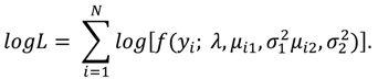
The PAE of [12] is based on the extremely flexible mixture of (two) normal distributions. A mixture of two normal distributions is a random variable whose density function is a weighted sum of two normal density functions. To obtain the density function of a mixture, let φ denote the density function of a normal distribution with mean µ and variance σ2,
 while Φ represents the cumulative distribution function of the standard normal. Then, the density function of a mixture of two normal distributions, the case most often examined, is given by,
where 0 ≤ λ ≤1. The cumulative distribution function of a mixture of two normal distributions is given by,
while Φ represents the cumulative distribution function of the standard normal. Then, the density function of a mixture of two normal distributions, the case most often examined, is given by,
where 0 ≤ λ ≤1. The cumulative distribution function of a mixture of two normal distributions is given by,
f(x: λ,μ1,σ12,μ2,σ22 ) = λϕ(x: μ1,σ12 ) + (1 - λ)ϕ(x: μ2,σ22 )
Henceforth, we use f and F to indicate the density and cumulative distribution functions, respectively, of a mixture of two normal distributions.
A mixture of two normal distributions has several advantages in partially adaptive estimation. First, a mixture of two normals contains the normal as a special case which facilitates comparisons with the common formulation of most limited-dependent variable (LDV) models. In this case, the grouped-data regression model is contained in the partially adaptive model. Second, a mixture of two normals is more flexible than partially adaptive approaches based on generalizations of the t-distribution. In particular, a mixture of two normal distributions can accommodate every possible combination of skewness and kurtosis. Third, the approach can easily be extended to more than two normal distributions. For applications of a mixture of normal regressions [34,35], see Beard, Caudill and Gropper [34] and Caudill, Gropper and Hartarska [35].
In order to develop a PAE based on a mixture of normals for the grouped-data regression model, a result from Bartolucci and Scaccia [28] is needed. Using their notation, we begin with the usual regression model relating a dependent variable, y, to several independent variables, Xi,
yi = α + Xiβ + εi
Following [28], let,
μi = α + Xiβ
Then, the density function of yi based on the normality assumption is given by,
The log-likelihood function to be maximized in this case is,
Equations (2) through (5) provide the framework for ML estimation of the linear model. Bartolucci and Scaccia extend this approach to a flexible alternative which is a mixture of two normal regression models with the slope coefficients constrained to be equal across regimes, yet allowing for the intercepts to vary. The result is essentially two parallel regression models. To extend the usual regression model, following [28], let the regression coefficients in the mixture be given by,
μij = αj + Xiβ
where i indicates observation: i =1 to N and j indicates regime, j=1,2. The density from Bartolucci and Scaccia is then,
f(yi; λ,μi1,σ12,μi2,σ22 ) = λϕ(yi; μi1,σ12 ) + (1 - λ)ϕ(yi; μi2,σ22 )
where λ is the mixing weight with 0 ≤ λ ≤ 1. The log-likelihood function is then,
Equations (6) through (8) give the framework for ML estimation of the linear model following the approach detailed by [28]. The likelihood function in (8) can be maximized by using the expectations maximization, or EM, algorithm given by Bartolucci and Scaccia. Although the approach based on mixture adds flexibility, the added flexibility comes at a cost. Compared to the usual ML estimator of the simple linear regression model, three additional parameters must be estimated: the mixing weight, an intercept, and a variance.
The approach of Bartolucci and Scaccia is extended to the grouped-data regression model by Caudill and Long [12]. Below we derive the usual grouped-data regression model and then the partially adaptive extension. The latent variable regression model is given by,
yi* = α + Xiβ + εi
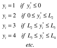
where ε is normally distributed with mean zero and variance σ2, while the interval endpoints are,

with L0 = -∞, L1 = 0, and LK = ∞. Thus, observed y is related to y* as follows:
Regression parameters are estimated by ML based on products of probabilities such as,

The log-likelihood function is given by,
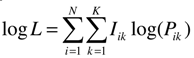
where Iik is a set of dummy variables for each observation i, such that Iik equals 1 if the ith observation is in the kth interval, and 0 otherwise.
The partially adaptive approach of [12] is based on a mixture of two normal distributions. Probabilities of interval membership are given by,
Pik = prob(yi = k) = F[Lk] - F[Lk-1]
The log-likelihood function is given by,
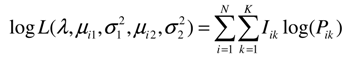
The model is estimated by ML using the EM algorithm given in Caudill and Long [12]. Our results are based on both the usual grouped-data regression model and the partially adaptive approach of Caudill and Long [12]. 1 Estimated coefficients in the grouped data regression model and in the partially adaptive regression model are interpreted just like their OLS counterparts; that is, they are marginal effects.
5. Results
Summary statistics for our samples are given in Table 1. The means and standard deviations for 2011 are given in column two of the table and the means and standard deviations for 2012 are given in column three of the table. There is little difference in the means of variables between the two years except for two cases; Stoppage_sec and NATV. Stoppage_sec is the reported stoppage time, which is about 26 seconds more in the 2012 season than in 2011. Also, in 2012 the fraction of matches that were nationally televised is 0.334, up from 0.258 in 2011.
We turn now to a discussion of our estimation strategy. We estimate our models using grouped data regression, then test down using likelihood ratio tests to obtain a parsimonious model which is ultimately estimated using the partially adaptive approach of Caudill and Long [12]. Using a general-to-specific modeling approach, we estimate Equation (1) above for 2011 and 2012. Our first step is to test for the presence of referee fixed effects and drop them from the model if the null hypothesis that all associated coefficients equal zero cannot be rejected.2 We do the same for the venue fixed effects. If, in either case, the null is rejected, we use a forward stepwise procedure to determine which fixed effects to include.3 We also test for the presence of a home field advantage by jointly testing the coefficients of Behind1, Behind2, and Waybehind. If the null cannot be rejected, we omit the group. If the null can be rejected, we retain the entire group in future specifications.
5.1. The 2011 Season
We estimate the model in Equation (1) for second half stoppage time in 2011 first. First, we test the null hypothesis that the coefficients of all of the referee fixed effects are zero. We cannot reject this hypothesis. The resulting chi-square is 29.19 with 25 degrees of freedom, resulting in a p-value of 0.26. We test the null hypothesis that the coefficients of all of the venue fixed effects are zero. We cannot reject this hypothesis. The chi-square value is 16.39 with 19 degrees of freedom, yielding a p-value of 0.63. We test the null hypothesis that the coefficients of all of the “home bias” coefficients are zero. We cannot reject this hypothesis. The chi-square value is 1.48 with 3 degrees of freedom, yielding a p-value of 0.69. The referee fixed effects, the venue fixed effects, and the home bias dummy variables are omitted from subsequent estimations.

Table 1.
Sample means and standard deviations for 2011 and 2012 Major League Soccer (MLS) seasons.
| Variable | 2011 | 2012 |
|---|---|---|
| Stoppage_sec | 260.000 (74.96) | 285.882 (85.39) |
| Yellow | 1.837 (1.28) | 1.854 (1.30) |
| Red | 0.170 (0.43) | 0.115 (0.35) |
| Subs | 4.725 (1.01) | 4.864 (1.08) |
| Tied | 0.386 (0.489) | 0.402 (0.49) |
| Diff1 | 0.471 (0.50) | 0.421 (0.49) |
| Diff2 | 0.118 (0.32) | 0.149 (0.36) |
| Bigdiff | 0.026 (0.16) | 0.028 (0.16) |
| Behind1 | 0.180 (0.38) | 0.017 (0.38) |
| Behind2 | 0.036 (0.19) | 0.046 (0.21) |
| Waybehind | 0.007 (0.08) | 0.006 (0.08) |
| AttPct | 0.771 (0.24) | 0.825 (0.25) |
| NATV | 0.258 (0.44) | 0.334 (0.47) |
We re-estimate the model with the omitted dummy variables. The results of estimating the model are given in Table 2. The OLS results, presented for comparison, are given in column two of the table. As the results are very similar to the grouped data results, we do not discuss them in detail here. Column three of the table contains the results from estimating the grouped-data regression model. Our earlier test indicated no evidence for a home bias in the awarding of stoppage time. The estimated coefficients of Tied, Diff1, and Diff2 (132.34, 111.68, and 103.92, respectively) are declining, which is consistent with close bias in that more stoppage time is added the closer the score at the end of regulation. We tested the equality of the coefficients using a likelihood ratio test and we can reject the null hypothesis of equality (χ2(3) = 25.88 with p-value = 0.00). We find no evidence that attendance as a fraction of stadium capacity has an impact on stoppage time. However, the coefficient of NATV indicates that nationally televised matches are, on average, about 22 seconds longer than untelevised matches (t = 2.32).
In order to make certain our findings are not an artifact of the normality assumption, we re-estimate the model using the partially adaptive approach detail earlier. We find that there is considerable evidence indicating that the underlying error structure is not normal. Following Sarstedt and Schwaiger (2008), we calculate Akaike’s Information Criterion (AIC), consistent Akaike’s Information Criterion (CAIC), Bayesian Information Criterion (BIC), and the sample-size adjusted AIC (ABIC) for the grouped-data regression model and our PAM estimator. We use these statistics in our application for model selection. All four information criteria favor the partially adaptive model over the usual grouped-data regression model. In addition, we plot the estimated density functions for the usual grouped-data regression and the partially adaptive version, evaluated at the sample means of the independent variables. The results are given in Figure 1, and do show that the mixture density is more compact than the normal with a fatter right tail. Clearly, the two distributions are different.
Table 2.
Estimation results for the 2011 MLS regular season.
| Variable | OLS Estimation Results1 | Grouped-Data Estimation Results2 | Partially Adaptive Estimation Results |
|---|---|---|---|
| Intercept 1 | 69.226 (1.90) | 99.208*** (2.76) | 100.382*** (3.65) |
| Intercept 2 | ------- | ------- | 85.777*** (3.45) |
| Yellow | 8.311 (2.60) | 8.312*** (2.64) | 7.098*** (3.00) |
| Red | 20.447 (2.11) | 20.440** (2.14) | 15.236** (2.29) |
| Subs | 14.113*** (3.44) | 14.127*** (3.48) | 9.010*** (2.94) |
| Tied | 132.338*** (5.07) | 132.354*** (5.14) | 151.508*** (10.10) |
| Diff1 | 111.678*** (4.34) | 111.660*** (4.40) | 139.084*** (9.52) |
| Diff2 | 103.92*** (3.74) | 103.892*** (3.80) | 138.688*** (8.75) |
| AttPct | -20.885 (1.20) | -20.943 (1.22) | -3.308 (0.26) |
| NATV | 21.851 (2.29) | 21.881** (2.32) | 12.143* (1.73) |
| Sigma1 | 70.360 | 67.233 | 108.255 |
| Sigma2 | ------- | ------- | 31.316 |
| Mixing weight | ------- | ------- | 0.331 |
| -ln L | ------- | 478.494 | 448.665 |
- 1
- Figures in parentheses are absolute values of t-ratios based on robust standard errors.
- 2
- Estimated coefficients in the grouped data regression model and in the partially adaptive regression model are interpreted just like their OLS counterparts; that is, they are marginal effects.
- ***
- Significant at the α = 0.01 level, two-tailed test.
- **
- Significant at the α = 0.05 level, two-tailed test.
- *
- Significant at the α = 0.10 level, two-tailed test.
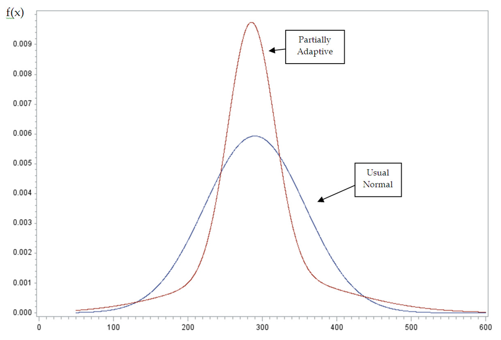
Figure 1.
2011. Densities of normal and mixture of normals
The estimation results for the partially adaptive version of our model are given in column four of Table 2. The results are similar to those obtained from the usual grouped data regression model. Like the grouped data regression model, the only coefficient not achieving statistical significance is that of AttPct. The coefficient of NATV is smaller in magnitude, but still indicates a statistically significant increase in stoppage time for nationally televised matches. The coefficient indicates about 12 additional seconds of stoppage time (with a t-ratio of 1.73).
5.2. The 2012 Season
One important difference in 2012 is that the broadcast networks changed somewhat; specifically, NBC entered the scene while FOX made an exit. Our analysis of the 2012 season proceeds similarly to that for 2011. We tested for referee and venue fixed effects. To begin, we return to our full model given in Equation (1) above. We can reject the null hypothesis of no referee fixed effects. The chi-square value is 54.44 with 30 degrees of freedom and a p-value of 0.001. The null hypothesis of no venue fixed effects cannot be rejected. The chi-square value is 24.26 with 18 degrees of freedom and a p-value of 0.15. We can reject the null hypothesis of no home field bias.4 The chi-square is 7.22 with 3 degrees of freedom and a p-value of 0.07.
Based on these test results, we omit the venue fixed effects from the model and retain our home field variables: Behind1, Behind2, and Waybehind. For the referee fixed effects, we conduct a forward stepwise procedure and admit a referee effect if the associated p-value is less than 0.10. This procedure resulted in the addition of seven referee dummy variables; Ref1, Ref6, Ref12, Ref22, Ref23, Ref28, and Ref30.
The OLS estimation results are given in column two of Table 3 and are presented for the purpose of comparison. Again, they are not discussed here as they are similar to the grouped data regression results. The grouped data estimation results are given in column three of Table 3. The coefficients of all variables except Red, Behind2, Waybehind, and AttPct are statistically significant at the α = 0.10 level or better. There are two main results for 2012. First, unlike 2011, there is a negative and significant national television effect. The coefficient is −18.88 with a t-ratio (absolute value) of 1.90. The other finding, consistent with most empirical studies on soccer, is the presence of a home field advantage. This conclusion is based on the coefficient of Behind1, indicating that an additional 29 seconds of stoppage time (t = 2.20) is added if the home team, rather than the visiting team, is behind by one goal at the end of regulation play.5
As before, we also estimate the partially adaptive model in case our results are due to the restrictive normality assumption in the grouped-data regression model. Several information criteria support the partially adaptive model over the usual grouped-data regression. Figure 2 contains plots of the normal and mixture-of-normals density functions evaluated at the sample means. The mixture-of-normals density looks much like that in the 2011 case. This density differs greatly from the normal, being more concentrated, shifted left, and having a fatter right tail.
The results of estimating the partially adaptive model are given in the fourth column of Table 3. These results mirror those from the grouped-data regression model, with two notable exceptions. There is now a statistically significant home field advantage if the home team is behind by more than two goals at the end of regulation play. The coefficient indicates that about 80 additional seconds of stoppage time are added if the home team is way behind the visiting team (t = 1.98). The national television effect is now highly insignificant. The important finding of an additional 25–30 seconds of stoppage time added when the home team is behind by one goal remains.
Table 3.
Estimation results for the 2012 MLS regular season.
| Variable | OLS Estimation Results1 | Grouped-Data Estimation Results2 | Partially Adaptive Estimation Results |
|---|---|---|---|
| Intercept1 | 71.321* (1.79) | 108.274*** (2.81) | 171.205*** (4.60) |
| Intercept2 | ------- | ------- | 129.599*** (4.03) |
| Yellow | 11.913*** (3.48) | 11.614*** (3.52) | 11.919*** (4.25) |
| Red | -1.041 (0.08) | -2.468 (0.20) | 6.528 (0.58) |
| Subs | 13.314*** (3.29) | 12.537*** (3.19) | 8.665*** (2.82) |
| Tied | 136.036*** (4.48) | 134.166*** (4.57) | 120.529*** (4.86) |
| Diff1 | 97.818*** (3.17) | 97.104*** (3.26) | 96.473*** (3.82) |
| Diff2 | 93.764*** (2.87) | 92.188*** (2.92) | 90.153*** (3.35) |
| Behind1 | 29.315* (2.16) | 28.962** (2.20) | 25.855** (2.23) |
| Behind2 | 25.749 (1.05) | 26.547 (1.12) | 9.303 (0.48) |
| Waybehind | 86.392 (1.39) | 91.844 (1.52) | 82.856* (1.98) |
| AttPct | 13.570 (0.78) | 17.717 (1.05) | 1.355 (0.10) |
| NATV | -6.084 (0.64) | -16.877* (1.90) | -1.556 (0.20) |
| Ref1 | 129.894 (3.69)*** | 127.051*** (3.74) | 92.877*** (4.18) |
| Ref6 | 55.325* (1.84) | 55.285* (1.90) | 41.023* (1.74) |
| Ref12 | 91.497** (2.61) | 92.949*** (2.76) | 23.224 (1.07) |
| Ref22 | -32.403* (1.74) | -31.936* (1.78) | -25.008 (1.60) |
| Ref23 | -134.458*** (2.43) | -138.055*** (2.58) | -130.069*** (3.94) |
| Ref28 | 64.318** (2.15) | 63.625** (2.20) | 73.532*** (3.43) |
| Ref30 | -59.915* (1.99) | -60.103** (2.06) | -33.765*** (3.43) |
| Sigma1 | 76.899 | 72.263 | 115.606 |
| Sigma2 | ------- | ------- | 43.570 |
| Mixing weight | ------- | ------- | 0.273 |
| -lnL | ------- | 527.183 | 508.723 |
- 1
- Figures in parentheses are absolute values of t-ratios based on robust standard errors.
- 2
- Estimated coefficients in the grouped data regression model and in the partially adaptive regression model are interpreted just like their OLS counterparts; that is, they are marginal effects.
- ***
- Significant at the α = 0.01 level, two-tailed test.
- **
- Significant at the α = 0.05 level, two-tailed test.
- *
- Significant at the α = 0.10 level, two-tailed test.
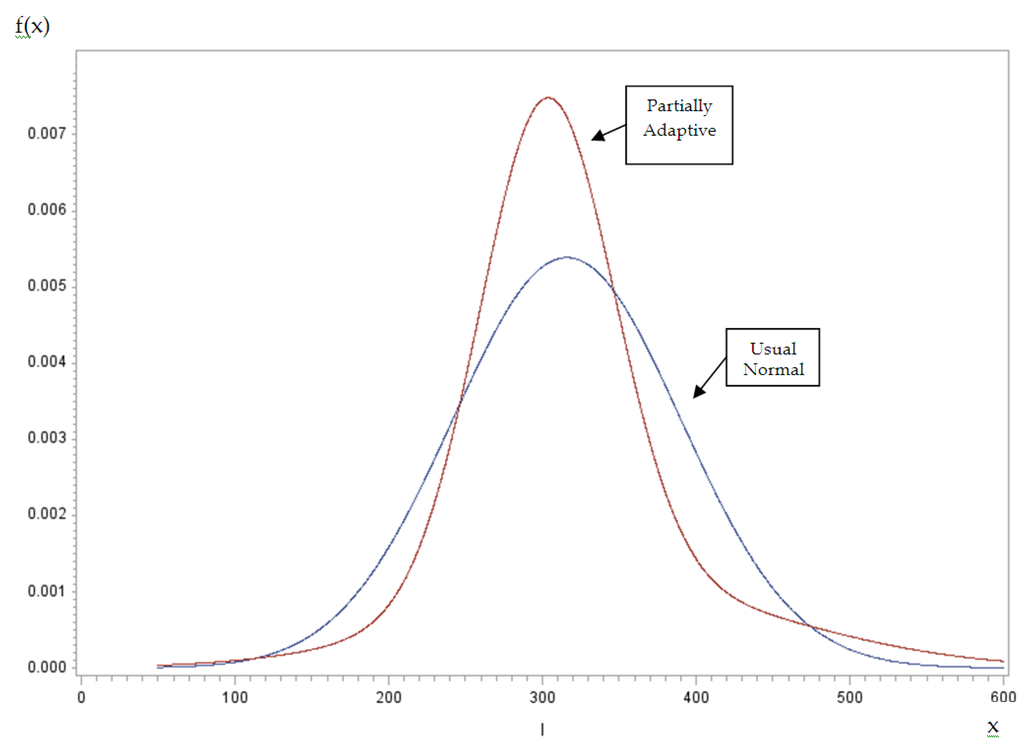
Figure 2.
2012. Densities of normal and mixture of normals.
The results from the 2011 and 2012 seasons have little in common. There is no home field advantage in the addition of stoppage time in 2011, but this often-found effect is present in 2012. There is a national television effect in 2011, but not in 2012. If one looks simply at the means of stoppage time, nationally televised matches are, on average, about 14 seconds longer than other matches. In 2012, nationally televised matches are, on average, about 14 seconds shorter than other matches. However, average stoppage time in 2012 exceeded average stoppage time in 2011. In fact, although the average stoppage time for a nationally televised match is not much different in 2011 than in 2012, the big change is in the stoppage time for the other matches. For those matches not nationally televised, the average stoppage time in 2012 is over 33 seconds longer than the average in 2011.6 The “nationally televised” effect is not statistically significant in 2012, indicating that differences in the other independent variables in the model accounted for the spread. That is not the case in 2011, as the effect is statistically significant, ceteris paribus. One possible explanation for the finding is that 2011 is the year that the MLS contract with FOX ended, and that some longer matches might have put MLS in a better negotiating position against FOX and/or NBC.
6. Conclusions
This study examines home bias, close bias, and television bias in Major League Soccer (MLS) using data on second-half stoppage time for the 2011 and 2012 MLS seasons. There are several novel features of our study. We use data from the two most recent MLS seasons, 2011 and 2012. We include a dummy variable to investigate the existence of a television effect on stoppage time. We note that reported stoppage time is interval-censored and, consequently, we estimate a grouped-data regression model. We also estimate a partially adaptive regression model, following [12].
Our findings indicate that there is no home field advantage in the awarding of stoppage time in 2011. We do find a positive television effect on stoppage time. In particular, from 12 to 23 seconds more stoppage time is added for a nationally televised match, ceteris paribus. Our results for 2012 more closely resemble previous work on stoppage time in soccer. We do find evidence of a home field advantage. In particular, if the home team is behind by one goal at the end of regulation, about 33 seconds of stoppage time is added beyond the average for a visiting team facing a one-goal deficit. We find no evidence of a television bias in 2012. One possible explanation for the reversal, certainly as far as the impact of television is concerned, is that MLS’ contract with FOX expired in 2011, and it was in the process of being renegotiated with FOX’s rival NBC. Longer matches might translate into more viewers of MLS matches, and, as a result, a more favorable television contract for MLS.
Acknowledgments
The authors thank two anonymous referees for helpful comments on previous versions of this study, and Greg Lalas, Editor-in-Chief of MLSSoccer.com, for providing the data used in this study. The usual caveat applies.
Conflicts of Interest
The authors declare no conflict of interest.
References
- T.J. Moskowitz, and L.J. Wertheim. Scorecasting: The Hidden Influences behind how Sports are Played and Games are Won. New York, NY, USA: Crown Publishing, 2011. [Google Scholar]
- M. Sutter, and M.G. Kocher. “Favoritism of agents—The case of referees’ home bias.” J. Econ. Psychol. 25 (2004): 461–469. [Google Scholar] [CrossRef]
- V. Scoppa. “Are subjective evaluations biased by social factors or connections? An econometric analysis of soccer referee decisions.” Empir. Econ. 35 (2007): 123–140. [Google Scholar] [CrossRef]
- L. Garicano, I. Palacios-Huerta, and C. Prendergast. “Favoritism under social pressure.” Rev. Econ. Stat. 87 (2005): 208–216. [Google Scholar] [CrossRef]
- P. Dawson, and S. Dobson. “The influence of social pressure and nationality on individual decisions: Evidence from the behavior of referees.” IASE/NAASE Working Paper No. 08-09, 2008. [Google Scholar]
- N. Rickman, and R. Witt. “Favouritism and financial incentives: A natural experiement.” Economica 75 (2008): 296–309. [Google Scholar] [CrossRef]
- T. Dohmen. “The influence of social forces: Evidence from the behavior of football referees.” Econ. Inq. 46 (2008): 411–424. [Google Scholar] [CrossRef]
- P. Pettersen-Lidbom, and M. Priks. “Behavior under social pressure: Empty italian stadiums and referee bias.” Econ. Lett. 108 (2010): 212–214. [Google Scholar] [CrossRef]
- B. Buraimo, D. Forrest, and R. Simmons. “The 12th man? Refereeing bias in English and German soccer.” J. Royal Stat. Soc. 173 (2010): 431–449. [Google Scholar] [CrossRef]
- B. Buraimo, R. Simmons, and M. Maciaszczyk. “Favoritism and referee bias in european soccer: Evidence from the Spanish league and the UEFA Champions League.” Contemp. Econ. Pol. 30 (2012): 329–343. [Google Scholar]
- J. Price, M. Remer, and D.F. Stone. “Subperfect game: Profitable biases of NBA referees.” J. Econ. Manag Strateg. 21 (2012): 271–300. [Google Scholar] [CrossRef]
- S.B. Caudill, and J.E. Long. “Do former athletes make better managers? Evidence from a partially adaptive grouped-data regression model.” Empir. Econ. 39 (2010): 275–290. [Google Scholar] [CrossRef]
- Fédération Internationale de Football Association (FIFA), ed. The Official Laws of the Game. Chicago, IL, USA: Triumph Books, 1991.
- R. Sandomir. “U.S. pro league moves along by signing a television deal.” New York Times. Available online: http://www.nytimes.com/1994/03/16/sports/soccer-us-pro-league-moves-along-by-signing-a-television-deal.html (accessed 16 March 1994).
- J. Ourand. “NBC signs three-year deal with MLS for FOX Soccer’s television package.” Street & Smith’s Sports Business Daily. Available online: http://www.sportsbusinessdaily.com/Daily/Issues/2011/08/10/Media/MLS-NBC.aspx (accessed 10 August 2011).
- “Staff ESPN purchases broadcast rights to MLS games.” Available online: http://espnfc.com/news/story?id=375076&cc=5901 (accessed 5 August 2006).
- T. Mickle, and J. Ourand. “ESPN booting MLS from its Thursday slot.” Street & Smith’s Sports Business Daily. Available online: http://www.sportsbusinessdaily.com/Journal/Issues/2009/01/20090119/This-Weeks-News/ESPN-Booting-MLS-From-Its-Thursday-Slot.aspx. (accessed 19 January 2009).
- J. Bell. “MLS and NBC Sports announce new TV deal.” New York Times. Available online: http://goal.blogs.nytimes.com/2011/08/10/m-l-s-and-nbc-sports-announce-new-tv-deal/ (accessed 10 August 2011).
- E. Spanberg. “Soccer’s new stage.” Street & Smith’s Sports Business Daily. Available online: http://www.sportsbusinessdaily.com/Journal/Issues/2012/03/05/In-Depth/MLS-NBC.aspx (accessed 5 March 2012).
- M.B. Stewart. “On least squares estimation when the dependent variable is grouped.” Rev. Econ. Stud. 50 (1983): 737–753. [Google Scholar] [CrossRef]
- S.B. Caudill. “More on grouping coarseness in linear normal regression models.” J. Econom. 52 (1992): 407–417. [Google Scholar] [CrossRef]
- J.E. Long, and S.B. Caudill. “The impact of participation in intercollegiate athletics on individual income and graduation.” Rev. Econ. Stat. 73 (1991): 525–531. [Google Scholar] [CrossRef]
- J.B. McDonald, and W.K. Newey. “Partially adaptive estimation of regression models via the generalized T distribution.” Econom. Theory 4 (1988): 428–457. [Google Scholar] [CrossRef]
- R.J. Butler, J.B. McDonald, R.D. Nelson, and S.B. White. “Robust and partially adaptive estimation of regression models.”.” Rev. Econ. Stat. 2 (1990): 321–327. [Google Scholar]
- J.B. McDonald, and S.B. White. “A comparison of some robust, adaptive, and partially adaptive estimators of regression models.” Econom. Rev. 12 (1993): 103–124. [Google Scholar] [CrossRef]
- R.F. Phillips. “A constrained maximum likelihood approach to estimating switching regressions.” J. Econom. 48 (1991): 241–262. [Google Scholar] [CrossRef]
- R.F. Phillips. “Partially adaptive estimation via a normal mixture.” J. Econom. 64 (1994): 123–144. [Google Scholar] [CrossRef]
- F. Bartolucci, and L. Scaccia. “The use of mixtures for dealing with non-normal regression errors.” Comput. Stat. Data Anal. 48 (2005): 821–834. [Google Scholar] [CrossRef]
- X. Wu, and T. Stengos. “Partially adaptive estimation via the maximum entropy densities.” Econom. J. 9 (2005): 1–15. [Google Scholar]
- J.B. McDonald. “An application and comparison of some flexible parametric and semi-parametric qualitative response models.” Econ. Lett. 53 (1996): 145–152. [Google Scholar] [CrossRef]
- J. Geweke, and M. Keane. “Mixture-of-normals probit. Federal Reserve Bank of Minneapolis.” Research Staff Report 237. August 1997. [Google Scholar]
- J.B. McDonald, and Y.J. Xu. “A comparison of semi-parametric and partially adaptive estimators of the censored regression model with possibly skewed and leptokurtic error distributions.” Econ. Lett. 51 (1996): 153–159. [Google Scholar]
- S.B. Caudill. “A partially adaptive estimator for the censored regression model based on a mixture of normal distributions.” Stat. Methods Applic. 21 (2012): 121–137. [Google Scholar] [CrossRef]
- T.R. Beard, S.B. Caudill, and D.M. Gropper. “Finite mixture model estimation of multi-product cost functions.” Rev. Econ. Stat. 73 (1991): 654–664. [Google Scholar] [CrossRef]
- S.B. Caudill, D.M. Gropper, and V. Hartarska. “Which microfinance institutions are becoming more cost-effective with time? Evidence from a mixture model.” J. Money Credit Bank. 41 (2009): 651–672. [Google Scholar] [CrossRef]
- M. Sarstedt, and M. Schwaiger. “Model selection in mixture regression analysis—A Monte Carlo simulation study.” In Data Analysis, Machine Learning and Applications: Proceedings of the 31st Annual Conference of the Gesellschaft für Klassifikation e.V., Albert-Ludwigs-Universität Freiburg, 7–9 March 2007; 2008, pp. 61–68. [Google Scholar]
- 1All partially adaptive models are estimated using a program written by the authors in the IML language in SAS that is available from the authors upon request.
- 2Alternatively, one could estimate a mixed model but the software does not presently exist to estimate a partially adaptive interval-censored mixed model.
- 3We are grateful to an anonymous referee for this suggestion.
- 4Following a suggestion of a referee, we also tested for home bias by replacing Behind1, Behind2, and Waybehind with the interaction terms AttPct*Behind1, AttPct*Behind2, and AttPct*Waybehind in our models for 2011 and 2012. Our conclusions regarding the absence of home bias in 2011 and the presence of home bias in 2012 were unchanged.
- 5Given that the law governing stoppage time allows referees to account for “wast[ed] time” during regulation play, it is possible that numerous excessive goal celebrations could account for some of the observed stoppage time in a given soccer contest. To account for this, we constructed and added the total number of second-half goals scored to the set of regressors from our most general grouped-data regression model. For 2011, the estimated coefficient on this regressor is 1.05, with a t-ratio of 0.27. For the 2012, the estimated coefficient is −6.08 with a t-ratio of 1.29 (absolute value). Thus, the variable is not significant.
- 6Following the suggestion of a referee, we pooled the 2011 and 2012 data and then divided the sample into nationally televised and not nationally televised matches. We returned to our large model (1), dropped NATV and added a year dummy variable for 2012. For the televised games we found no evidence of a home field advantage. Although the Behind1 coefficient was marginally significant, the “home” group was not (χ2(3) = 3.62 with p-value = 0.3057). For the matches not nationally televised we found some evidence of a home field advantage, surprisingly based on the strength of a large positive and statistically significant Waybehind coefficient. Testing our “home” group here gave a χ2(3) = 7.69 with a p-value of 0.0528. This is consistent with our prior belief that close bias is more important for televised games and home bias is more important for not-televised games.
© 2014 by the authors; licensee MDPI, Basel, Switzerland. This article is an open access article distributed under the terms and conditions of the Creative Commons Attribution license (http://creativecommons.org/licenses/by/3.0/).