Abstract
Large-scale population flow reshapes the economic landscape and is affected by unbalanced urban development. The exploration of migration patterns and their determinants is therefore crucial to reveal unbalanced urban development. However, low-resolution migration datasets and insufficient consideration of interactive differences have limited such exploration. Accordingly, based on 2019 Chinese Spring Festival travel-related big data from the AMAP platform, we used social network analysis (SNA) methods to accurately reveal population flow patterns. Then, with consideration of the spatial heterogeneity of interactive patterns, we used spatially weighted interactive models (SWIMs), which were improved by the incorporation of weightings into the global Poisson gravity model, to efficiently quantify the effect of socioeconomic factors on migration patterns. These SWIMs generated the local characteristics of the interactions and quantified results that were more regionally consistent than those generated by other spatial interaction models. The migration patterns had a spatially vertical structure, with the city development level being highly consistent with the flow intensity; for example, the first-level developments of Beijing, Shanghai, Chengdu, Guangzhou, Shenzhen, and Chongqing occupied a core position. A spatially horizontal structure was also formed, comprising 16 closely related city communities. Moreover, the quantified impact results indicated that migration pattern variation was significantly related to the population, value-added primary and secondary industry, the average wage, foreign capital, pension insurance, and certain aspects of unbalanced urban development. These findings can help policymakers to guide population migration, rationally allocate industrial infrastructure, and balance urban development.
1. Introduction
Population flow refers to the short-term, repetitive, and cyclical movement of populations in geographical space. By 2016, China’s floating population had reached 245 million. Large-scale population flow has been a significant phenomenon in China’s social development and will continue to be so in the future [1]. Population flow is closely relevant to disease control, sustainable social development, congestion alleviation, information propagation, and e-commerce [2,3,4]. Determining the relationship between population migration and unbalanced urban development is key to ensuring sustainable social development.
Population flow represents the reallocation of production factors in space [5]. The greater the population flow, the greater the economic vitality [6]. Thus, population flow reflects the developmental level of a region or city [7]. Determining population flow patterns from spatiotemporal population behavior may therefore reveal developmental differences between cities. Population mobility is a social expression of the spatial interaction between an origin city and a destination city and is affected by unbalanced urban development. For example, cities with better economic conditions are more attractive to laborers from relatively poor urban areas [8]. As differences in urban development throughout China increase, population flow has become polarized. The stronger the economic vitality of an area, the greater the flow of population into it. Such enormous population flow has a severe effect on stable development in China. Therefore, quantification of the effect of socioeconomic factors on migration patterns is essential to improve regional development.
Large-scale intercity population flow occurs mainly during public holidays in China. The largest family reunion holiday in China is the Spring Festival, which in 2018 involved the travel of more than seven times the number of people who traveled during Thanksgiving in the United States in 2017 [9]. According to a report from the National Tourism Administration in China, 386 million people traveled during the Spring Festival of 2018. In addition, many people traveled between their work city and hometown during the Spring Festival, which is an event called “ChunYun”. This phenomenon enabled us to study spatiotemporal migration patterns and their determinants. However, it is difficult to collect detailed spatiotemporal data on large-scale population migration, which has led previous researchers to concentrate on the Yangtze River Delta, the Pearl River Delta, and the Beijing–Tianjin–Hebei urban agglomeration and megalopolises, so small and medium-sized cities are often not considered. However, differences in inter-regional interactions give poor estimates of global parameters for use in traditional spatial interaction models. This has limited the exploration of population flow patterns and the timely, accurate, and dynamic quantification of their effects.
This study aimed to comprehensively re-examine population flow patterns and their determinants. Most importantly, a family of spatially weighted interactive models (SWIMs) are applied to quantify the impact of socioeconomic factors on population mobility and reveal the urban issues of unbalanced development. To more accurately determine population flow and avoid spatiotemporal mismatch, we collected a population migration dataset from the AMAP platform and divided it into four subsets (daily, returning hometown, holiday, and returning work) according to the Spring Festival time nodes. Based on the daily subset, the PageRank algorithm, and the Clauset–Newman–Moore (CNM) algorithm, social network analysis (SNA) methods were used to reveal patterns. Based on the returning work subset, we used a family of spatial interaction models, comprising the global Poisson gravity model, origin-specific and destination-specific models, and SWIMs, to quantify the global and local effects of socioeconomic factors on returning work flow. When these advanced SWIMs are applied to study large-scale population flow, they have excellent performance of accounting for local effects in spatial interaction modeling.
2. Related Literature
Many influential theories and models have been proposed to explain the origin, mechanism, and extension of population migration, such as the “push and pull theory” [10]. Based on these theories, various regional disparities are regarded as creating complex motivations for migration. The explanation of migration patterns aids the understanding of demographic change and associated socioeconomic development. Therefore, migration within China has been studied by many scholars, with a focus on its spatial patterns and influencing factors.
Previous migration studies have been based on 10-yearly census data and annual interprovincial population flow data. Moreover, these studies involved limited data collection methods and thus, were mostly of low accuracy and long update times or based on only origin or destination attributes [11,12]. However, the rapid development of information communications technology and mobile applications makes it possible to track the spatiotemporal behaviors of large numbers of individuals. Many scholars have focused on a more comprehensive and detailed examination of population mobility at the national or provincial level and at the city level across China. Based on travel big data, Yang et al. analyzed the spatiotemporal patterns of population mobility and its determinants in Chinese cities, and Cui et al. analyzed the spatiotemporal dynamics of daily intercity mobility in the Yangtze River Delta [13,14]. The resulting data exhibit more spatiotemporality than previous data and can be integrated with external geographic factors to solve the problem of low spatiotemporal detail in related studies.
Nevertheless, it remains challenging to identify intercity flow patterns and efficiently quantify the effect of socioeconomic factors on migration patterns. Cities are the foci of regional economy, politics, culture, and transportation and attract people from surrounding areas due to their better employment opportunities, modern infrastructure, good educational environment, advantageous location, and efficient transportation [15]. Some cities have even developed into urban agglomerations that spread across surrounding areas, such as those of New York, London, Tokyo, Jiangsu–Zhejiang–Shanghai, and Beijing–Tianjin–Hebei. Other cities have formed complex social networks connected by mobile populations, with different population flow patterns to those of urban agglomerations. Traditional network analysis models have ignored the social attributes of population flow. Moreover, traditional spatial interaction models do not sufficiently consider differences in migration patterns because these models are based on global parameter estimation.
With the development of SNA methods, it has become popular to explore network node importance and network structure to determine flow patterns. For example, a large number of studies have applied SNA methods for pattern identification [16,17]. The PageRank algorithm has also been used to measure node importance in networks [18], and community detection has been used to find city communities [19]. These have developed a new approach for identification of the spatiotemporal patterns of large-scale population flow.
However, SNA methods only reveal flow network characteristics; they are unable to quantify the interaction of socioeconomic factors with population flow. Thus, the gravity model, which is a key spatial interaction model inspired by gravity or push–pull theories, and its related family of models have often been used to explain the interaction process [20]. Chen et al. used an improved gravity model to analyze a complex interprovincial mobile population network, and Zhang et al. implemented a new multilevel gravity model to study interprovincial urban migration flows [21,22]. A gravity model has also been calibrated globally, with one set of parameter estimates determined for a study region, followed by global parameter estimates. These global estimates were considered to represent the average interaction behavior and to be equally valid across the entire study area [23].
Thus, these gravity models ignored the local characteristics of population flow and failed to consider spatial heterogeneity. This problem has been addressed by separate modeling of each specific origin or destination city in a flow network to generate origin-specific and destination-specific spatial interaction models [24]. However, these models ignore the influence of surrounding cities on each specific origin or destination city and fail to capture local effects well. This problem is solved by geographically weighted regression (GWR), a technique that has become increasingly popular for detecting spatial nonstationarity in spatial analysis [25,26]. By combining GWR with a gravity model, Kordi and Fotheringham constructed a family of SWIMs to detect, visualize, and analyze spatial nonstationarity in spatial interaction processes [23]. Nevertheless, although these advanced SWIMs account for local effects in spatial interaction modeling, SWIMs have not been applied to the related study of large-scale population flow.
3. Study Area and Data
3.1. Study Area
There is large-scale population flow among cities in China during the Spring Festival. As portrayed in Figure 1, our study area focused on 299 prefecture-level administrative units and some county-level units in mainland China. In general, these administrative units are cities. Due to limitations in data availability, some prefecture-level cities in Hainan province, Taiwan, Hong Kong, Macao, and some ethnic minority autonomous prefectures in western China were excluded from the study area. Ultimately, 352 cities formed the research focus.
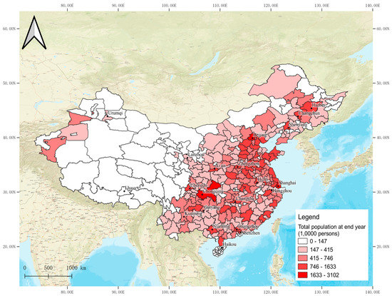
Figure 1.
Spatial distribution of study area (352 cities in total).
3.2. Study Data
Location-based services (LBS) technology pinpoints the geographic location of a mobile user via wireless communication networks or the external positioning methods of network operators. When users allow various mobile applications to call LBS, their movement trajectories are accurately recorded in real time from positioning information. Thus, every smartphone user is a mobile sensor, reflecting social characteristics and allowing an enormous amount of individual movement data to be collected efficiently in real time. These movement data are used to calculate intercity migration indices [27]. The use of travel-related big data with such high spatiotemporal resolution is more accurate and effective than the use of census data [28]. In this study, we used the population flow dataset from the AMAP Migration Map (“https://trp.autonavi.com/migrate/page.do”). Tencent and Baidu migration data have been used in similar studies because they provide migration indices of daily population inflows and outflows, with a city as the basic unit (i.e., the intensity of inflows, source, and outflows limited to the destination of a single city on a certain day). However, longer historical data for population migration, such as during the 2019 Spring Festival, are currently available only from the AMAP platform. Table 1 shows an example population flow dataset.

Table 1.
Example of a population flow dataset.
As shown in Table 1, the population migration intensity index (PMII; provided by the AMAP Migration Map) represents the migration intensity from the origin to the destination cities. In this study, the inflow and outflow migration indexes are both representative of the intensity of population flow.
In addition, to explore the effects of associated factors on the patterns of population flow during the Spring Festival, several socioeconomic factors were selected for analysis, as shown in Table 2. Thus, population is a basic factor in population flow; gross region product, value added by primary industry (VAPI), value added by secondary industry (VASI), and value added by tertiary industry (VATI) represent the economic level of cities; the average wage, in terms of the income differential between two cities, is the main driver of migration; foreign capital investment increases the number of jobs and thus, attracts employees; mobile phone users create a record of population movement, with their number closely related to the intensity of a population flow; and the number of insured pensions and insured persons (IPIP) represents the social security system for city workers and is an important indicator of the effect of social security policy on population flow.
Table 2.
Dependent and candidate independent variables used in the study.
Note: Variable means population migration intensity index of different period; Std. Dev. means standard deviation; Min means minimum value; Max means maximum value.For each city, we established indices to express the intensity of population flow (i.e., daily inflow and outflow) and the flows for holidays, returning to a hometown (re-hometown), and returning to work (re-work). From the spatiotemporal changes of these indices in the four periods, we determined the spatiotemporal trends and patterns of population flow. Because ChunYun began on January 21 during the Spring Festival of 2019, the average PMII distribution (DPMII) from January 15 to 20 was regarded as a proxy for the daily distribution of population flow before the Spring Festival. Similarly, the average PMII distribution (RHPMII) from January 21 to February 2 was regarded as a proxy for the re-hometown distribution of population flow before the Spring Festival. The Spring Festival holiday ended on February 10, thus the average PMII distribution (HPMII) from February 3 to 9 was regarded as a proxy for the holiday distribution of population flow during the Spring Festival, and the average PMII distribution (RWPMII) from February 10 to 12 was regarded as a proxy for the re-work distribution of population flow after the Spring Festival. The basic statistical information of the intensity of population inflow and outflow during the four periods is shown in Table 3.
Table 3.
Basic statistical information of population inflow and outflow intensity.
4. Methods
We illustrate the methodology used in the study by using the example of population flow between the cities of Beijing and Shanghai. First, we used the city-level population flow dataset collected from the AMAP LBS platform and the socioeconomic factors dataset collected from the Urban Statistical Yearbook of China in 2019. These processes comprised the null value, error value, data standardization, dataset partition, spatialization, and other data preprocess. Second, we used SNA methods and spatial interaction models to explore the patterns and quantify the effects of population flow. Thus, we performed the following tasks. (1) We used the PageRank model for city classification and the CNM model for community detection during daily population flow. By using the PageRank model, it is possible to quantify which city is more important for Beijing and Shanghai. By using the CNM model, it is possible to determine which urban community Beijing and Shanghai belong to, respectively. (2) We used the spatiotemporal variation of flow intensity to reveal the trends of population flow. (3) We used a family of global interaction models (the global Poisson gravity model, the origin-specific gravity model, and the destination-specific gravity model) to quantify the global effect of selected socioeconomic factors on the returning work flow. For example, the global interaction models assumed that population flow between any city conform to the same pattern and that population flow between Beijing and Shanghai follow this pattern. (4) We used an origin-focused SWIM and a destination-focused SWIM to quantify the local effect, with consideration of spatial heterogeneity. For instance, when Beijing is the origin city and Shanghai is the destination city, the origin-focused SWIM can consider the influence of cities around Beijing on population mobility between these two cities, and the destination-focused SWIM can consider the influence of cities around Shanghai on population flow between these two cities. Figure 2 shows a flowchart for this study.
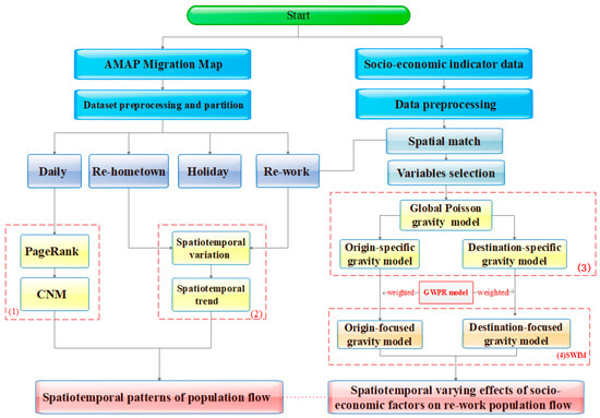
Figure 2.
Flowchart of this study (re-hometown means returning hometown; re-work means returning work; CNM means Clauset–Newman–Moore algorithm; GWPR means geographically weighted Poisson regression model; SWIM means spatially weighted interactive models).
4.1. City Classification and Community Detection
A population flow network is a small-world, scale-free network, an intermediate between a fully regular network and a completely random network [13]. We considered the network of population flow formed during the Spring Festival to be similar to the Internet and thus, considered that cities of greater importance attracted more people and routes. By taking cities as the network nodes and the intensity of population flow among cities as the weight, the following directional weighting matrix (P) for the four periods of population flow was constructed,
where resents the intensity of population flow from city i to city j.
To study the network characteristics of population flow, we used the PageRank algorithm and community detection methods, which are often used to measure node importance and community in SNA. The PageRank algorithm was originally designed to rank web pages by Google [39,40]. In addition to considering degree, betweenness, and closeness, like other centrality indices use to evaluate nodes in a network, the PageRank algorithm also considers the number and quality of connections. Thus, a node may have fewer connections yet still be important if its connections are with important nodes. The PageRank algorithm has therefore been applied to network analysis in many fields, such as bibliometrics, SNA, and road networks [13]. We used it to rank the importance of city nodes by classifying cities according to their importance, which revealed the hierarchical structure of population flow. The PageRank algorithm is as follows,
where is the PageRank value of city , q is a damping parameter for PageRank (usually set to 0.85), N is the number of all city nodes, represents the population flow from city to city , and is the number of links from city , which is weighted by the intensity of the population flow.
Community detection is used to identify city communities in a population flow network. A range of methods are used for community detection, such as the Fluid Communities algorithm, the Girvan–Newman algorithm, and the CNM algorithm [41,42,43]. We used the CNM algorithm, which is based on the CNM greedy modularity maximization and weighted by the intensity of a population flow [43].
4.2. Spatial Interaction Models
4.2.1. Global Poisson Gravity Model
Spatial interaction is broadly defined as the movement or communication of objects such as people, goods, and information over geographic space that results from a decision-making process [44,45]. Thus, spatial interaction covers a wide variety of behaviors and movements such as migration, shopping trips, commuting, commodity or communication flows, trips for educational purposes, and airline passenger traffic [23]. The most general form of a spatial interaction model can be formulated as follows [46],
where the interaction between any pair of origins and destinationsis specified as ,represents a vector of origin factors measuring the propulsiveness of origin , represents a vector of destination attractiveness factors, andrepresents a vector of separation factors, with the separation between city and (usually) measured in terms of distance, cost, or travel time between and . For example, is the population flow between Beijing and Shanghai. represents a vector of factors of Beijing, such as population and industry.represents a vector of factors of Shanghai, such as average wage and foreign investment.represents a vector of separation factors between Beijing and Shanghai, such as distance and transportation cost.
The gravity frameworks for spatial interaction were the first to be developed and are the most widely used [47]. The gravity model and its relationships assume that greater flows will occur between larger and closer places than between smaller and more distant places, ceteris paribus. It is usually formulated as follows,
where and represent the repulsiveness and attractiveness factors of origin and destination , respectively, is the distance between and and are parameters to be estimated empirically and that reflect the nature of the relationship between spatial flows and each of the explanatory variables [23].
Considering the Poisson regression, a global Poisson gravity calibration of spatial interaction models is formulated as follows,
where all parameters are as defined above.
4.2.2. Origin-Specific and Destination-Specific Models
Population flow is a spatial interaction between the population of the origin and the destination. Its intensity is affected by both the origin and the destination attributes, e.g., population mobility between Beijing and Shanghai is affected not only by the attributes of Beijing but also by those of Shanghai. However, as with the gravity model, the global calibration of spatial interaction models, which assumes the same pattern of the population flow between any origin and destination, may not capture the spatial variation in relationships and thus, may not represent the fact that the impact of Beijing and Shanghai is different.
Local parameter estimates may provide more useful disaggregated information. These estimates are obtained for each separate origin or destination by calibration of origin-specific and destination-specific models. For example, we only consider the flow from Beijing to any city in the origin-specific model, and we only consider the flow from any city to Shanghai in the destination-specific model.
An origin-specific model is formulated as follows,
where represents the flow intensity between the specific origin city and destination city ;,, and are the parameters of specific origin city represents a vector of destination attractiveness factors is the distance between and .
A destination-specific model is formulated as follows,
where represents the flow intensity between origin city and the specific destination city ,, and are the parameters of specific destination city represents a vector of origin factors measuring the propulsiveness of origin is the distance between and .
4.2.3. Origin-Focused and Destination-Focused Models
The origin-specific and destination-specific models only consider flows from a specific origin city to different destination cities or from different origin cities to a specific destination city. This means that flows emanating from other origins or arriving at other destinations are ignored. For example, in the origin-specific model, we only considered the flow from Beijing, but ignored the flow from other origin cities. In fact, the flow between origin and destination cities is affected by other cities that surround an origin and a destination. However, origin-specific and destination-specific models ignore this effect. Cities in various geographical locations have different population mobility patterns, whereas the mobility patterns of surrounding cities tend to be similar. Population flow is, therefore, spatially heterogeneous.
However, in the GWR model, a specific city is the research object, and the model generally performs better than traditional regression models because it includes geographically varying parameters. By using geographic weighting, it avoids the use of global parameter estimation, which renders traditional regression models unsuitable for analysis of spatially heterogeneous population flow patterns. The expression of the GWR model is as follows,
where are the coordinates of city and is the regression coefficient of independent variable at city , and the regression coefficient is the quantified result of the impact of each factor.
A weighted least-squares method is used to estimate the coefficients of the GWR model; the estimation of parameters can be given in the formula. The calculation of weight has a great influence on parameter estimation for the GWR model. A Gaussian kernel function is often used to calculate the spatially weighted matrix, which models the spatial effects of the surrounding observations by Gaussian distance decay within the bandwidth, as shown in Formula 10. Thus, bandwidth (b) selection is critical for the calculation of weight. There are two major categories of weighting methods: one uses a fixed bandwidth and the other uses an adaptive bandwidth. The bandwidth is larger when the data are sparse and in areas where the data are plentiful. Moreover, a corrected Akaike information criterion (AIC) is used to evaluate the fitting to select the optimum bandwidth [48].
where = diag(, , ,) is the spatially weighted matrix, and its diagonal elements (1 ≤ j ≤ n) are the weight given to observation city adjacent to observation city . It can be given as follows,
where is the spatial distance measuring the closeness between city and city , where b is a parameter called bandwidth, which is used to control the radial influence range.
GWR was initially developed for linear regression modelling, where the dependent variable is assumed to follow a Gaussian (normal) distribution. It was then extended to a geographically weighted logistic regression method, based on the generalized linear modelling framework for binomial (logistic) distribution and to a geographically weighted Poisson regression (GWPR) method, based on the Poisson distribution [49]. The expression of the GWPR model is as follows,
We used a geographically weighted likelihood principle to estimate the GWPR parameters. This is a variant of the local likelihood principle that is consistent with the geographically weighted least-squares approach of conventional Gaussian GWR. Thus, the model parameters at location were estimated by maximizing the geographically weighted log-likelihood function.
With reference to the geographical weighting approach used in the GWR model and the above models, SWIMs that included origin-focused and destination-focused models were constructed [23]. These also took focused cities as their research objects. In the origin-focused model, the flows with origins closer to the calibration point have a greater weight and thus, a larger effect during the model calibration. The weights continuously decrease as the distance between the calibration point and the observed origin increases. A simplified illustration of the origin-focused and destination-focused spatial interaction is shown in Figure 3.
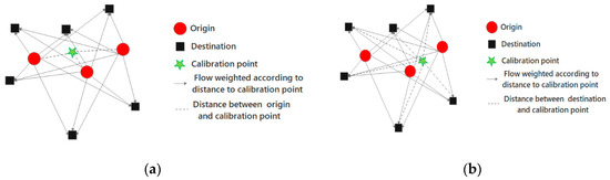
Figure 3.
A simplified illustration of the origin-focused and destination-focused models. (a) Origin-focused model, (b) Destination-focused model.
The general formulation of the SWIM is as follows,
where generally represents the flow intensity between origin city and destination city . When , the formulation is an origin-focused model, where represents the location of the calibration point (one of the existing origins or any other point within the study region); when , the formulation represents a destination-focused model, where represents the location of the calibration point (one of the existing destinations or any other point within the study region). The notation indicates that the data for the covariates obtained for the estimation of the parameters at are geographically weighted on the distances between and each , ,and , which are the model variables (i.e., the origin propulsiveness, the attractiveness of the destination, and the distance between origin and destination ) and and , which are the parameters specific to .
When the spatial interaction model follows a Poisson distribution, the SWIM is formulated as follows,
where denotes the flow between origin and destination weighted according to the distance between and , and other variables are defined as before.
The parameter estimation for the SWIM is similar to that used for the GWPR model, being based on a geographically weighted likelihood principle with pointwise-calibrated parameter estimates. A set of equations are solved to maximize the first derivative of the weighted log-likelihood in the SWIM, with these formulated as follows,
where indicates the weight of flow according to the proximity of its r to the calibration point u. The spatial weighting function and optimal bandwidth selection criteria of the SWIM are similar to those of the GWPR model.
4.2.4. Variables Selection
If there is multicollinearity in the regression models, the results will be highly unreliable. Thus, before modelling, it must be determined if multicollinearity exists between variables. We calculated the variance inflation factor (VIF) of each independent variable and discarded from the final model any independent variables with VIFs > 7.5, which were gross regional product of origin, gross regional product of destination, VATI_origin, VATI_destination, mobile phone users of origin, and mobile phone users of destination. The selected independent variables are shown in Table 4.
Table 4.
Variance inflation factor (VIF) value of selected independent variables.
5. Results
5.1. Spatiotemporal Patterns of Population Flow
Daily population flow exhibits spatiotemporality. As can be seen from Figure 4, the daily population flow is concentrated in the southeast of China, with little in the northwest of China. Furthermore, the deep red areas are four major city agglomerations, with Beijing, Shanghai, Guangzhou, and Chengdu as their respective core cities. These are known as Beijing–Tianjin–Hebei, the Yangtze River Delta, the Pearl River Delta, and Chengdu–Chongqing. In addition, the higher a city’s development level, the greater its population flow, as shown by the flow of Shanghai being greater than that of Chengdu. To verify this apparent hierarchical structure, we first established a directed weighted matrix of daily population inflow and outflow between cities, then used the PageRank algorithm to rank the importance of cities in the daily population flow network.
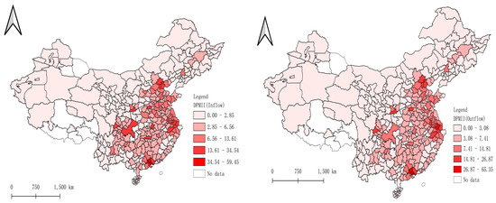
Figure 4.
Spatial distribution of daily population flow indices.
Figure 5 shows the PageRank value distribution of importance cities in different spatial locations, and Table 5 summarizes the levels of PageRank value in different cities by the natural break classification (NBC). The following trends can be seen: (1) the importance of first-level cities is consistent with that of the core cities of the four major city agglomerations mentioned above; (2) nearly all second-level cities are first-tier cities or provincial capitals, which are important nodes in the population flow network; (3) third-level cities surround a second-level city, showing that the intensity of population flow radiates from core cities to their surrounding cities, as mentioned above; and (4) the fourth-level cities are mainly distributed in northwestern China, which shows that the daily population flow is mainly concentrated in southeastern China. Thus, there is a vertical hierarchy, with the population flow showing a high consistency with city development level.
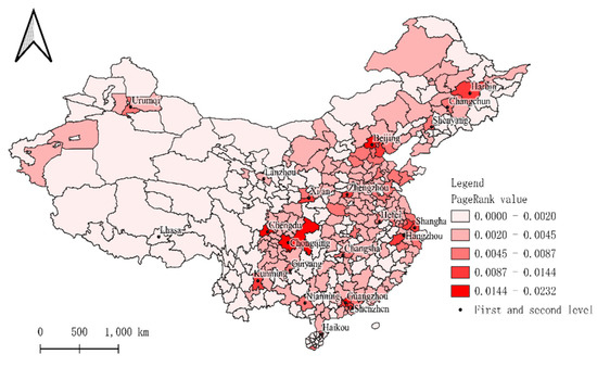
Figure 5.
Hierarchical map of cities in the population flow network.
Table 5.
Summary of city hierarchy in the population flow network.
The low-PageRanked cities surrounded high-level cities in geographical space; for example, Tianjin was one of the cities surrounding Beijing. This showed a possible community structure. Thus, community detection was used to reveal any community relationship that was hidden in the population flow network. Figure 6 gives a distribution map of the community structure in the network, and Table 6 summarizes the community structure of all cities. The latter reveals 16 different community structures and the following trends: (1) The core city of each community is a provincial capital city or municipality directly under central-government control; for example, the core city of the Beijing-related community is under central-government control. (2) The four major city agglomerations play an important role in the community structure, as they comprise the largest number of provinces and cities. (3) In the community structure, most communities are cross-regional, such as the Beijing-related community that encompasses Tianjin, Shandong, Shanxi, Hebei, and Henan provinces.
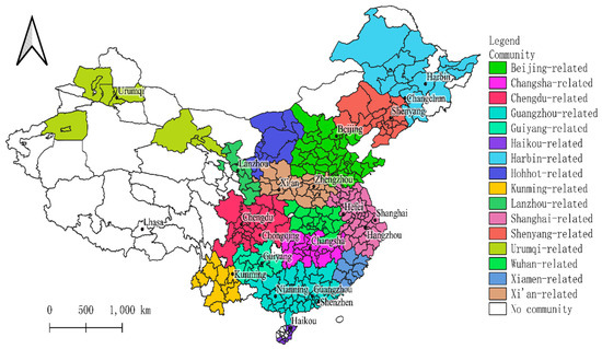
Figure 6.
Community map of cities in the population flow network.
Table 6.
Summary of the city community in the population flow network.
During the Spring Festival, as Table 3 shows, the mean increased from 4.505 to 10.82 and the mean increased from 4.496 to 10.75. Clearly, there was an overall increase in population flow. Further, Figure 7 is an outflow trend map of re-hometown before the Spring Festival, obtained by subtracting DPMII outflow from RHPMII outflow. The deep-red areas show a significant increase in outflow in four major city agglomerations. This is commonly known as “returning hometown flow” and represents migrant laborers returning to their hometowns to be with their families for the Spring Festival. Similarly, Figure 8 shows the inflow trend map of re-work after the Spring Festival obtained by subtracting HPMII inflow from RWPMII inflow. The deep-red areas show an inflow tendency to population flow in the four major city agglomerations, which represents migrant laborers returning to work after the Spring Festival (also denoted “returning work flow”). These data show that workers are concentrated mainly in the four major city agglomerations but that their hometowns are elsewhere. People therefore tend to flow from low-development cities to high-development cities, which have more employment opportunities.
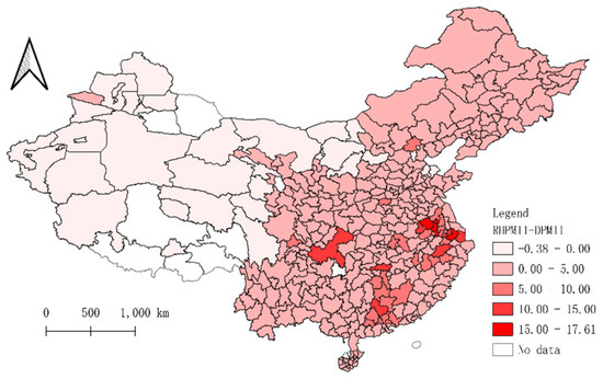
Figure 7.
An outflow trend map of re-hometown.
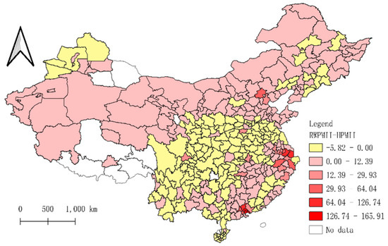
Figure 8.
Inflow trend map of re-work.
Overall, it was found that the spatiotemporal patterns of daily population flow had a hierarchical structure. Population flow intensity and city development were highly correlated and exhibited a community structure, indicating that the intensity of population flow radiated from core cities to surrounding cities. In terms of the hierarchical structure, the nationwide network level comprised the core cities (Beijing, Shanghai, Guangzhou, Chengdu, and Chongqing) of the four major city agglomerations; the regional network level comprised the second-level cities (e.g., Xi’an, Kunming, and Guiyang). In addition, there were more important and dense cities in eastern China than in western China, indicating a west-to-east flow of city development level in China. Cities in the same community tended to be more closely linked, indicating that they were connected by population flows more frequently than other cities. Moreover, most communities were cross-regional, illustrating that spatiotemporality will, in the future, be severely compressed: large-scale, cross-regional, and high-density population mobility will be a future development trend. During the Spring Festival, the spatiotemporal patterns of population flow were “returning hometown flow” and “returning work flow”. This verified the regional differences of city development and population flow. It also showed that the difference in developmental levels between two regions was the driving force of population flow. Large-scale population flow similar to “returning hometown flow” and “returning work flow” promotes the dissemination of information, capital, culture, and technology, which aids the development of cities.
5.2. SWIMs Result
The above analysis revealed that the unbalanced development of a city was an influential factor contributing to “returning hometown flow” and “returning work flow” during the Spring Festival. The migration purpose of “returning work flow” is to return to work. To account for the effect of multipurpose migration during daily and holiday periods, we used 13 explanatory variables to explore only the relationship between the intensity of population flow and the development level of a city during “returning work flow”. The dependent variable RWPMII and the independent variables are shown in Table 3.
5.2.1. Results from the Global Poisson Gravity Model
The parameter estimation result from the global Poisson gravity model is shown in Table 7. It represents only the average interaction behaviors across the entire study area. From the preliminary exploration, the following relationships can be seen. (1) The estimated value offor total population of origin is 0.7154, and that of of total population of destination is 0.1036, which shows that a population increase at origin and destination cities has positive effects on population flow. (2) The estimated value of for VAPI_origin (0.5019) indicates a positive effect on population flow but that of for VAPI_destination (−0.3018) indicates a negative effect. In contrast, the estimated value offor VASI_origin (−0.4667) indicates a negative effect on population flow but that of γ for VASI_destination (0.4400) indicates a positive effect. From the values for these four parameters, it can be concluded that primary-industry employment is saturated relative to secondary-industry employment at the global level. (3) The estimated values offor average wage of origin (0.7031402), of for average wage of destination (0.3977138), offor foreign capital of origin (0.0356023), and of for foreign capital of destination (0.0012664) are all positive. As neoclassical theorists have explained, the income level of an intended destination is the main driver of migration: thus, an income increase in the origin cities decreased the possibility of migrant worker outflow, while an income increase in the destination cities attracts more migrant workers. Further, foreign investment promotes economic development, provides more jobs, and attracts more migrant workers. (4) The estimated values offor IPIP_origin (−0.2480) indicate a negative effect on population flow, but the estimated values of IPIP_destination (0.4589) indicate a positive effect. This is in line with the actual situation: increased social security in origin cities results in more elderly workers not migrating, but a higher development level in destination cities increases social security and attracts more migrant workers.
Table 7.
Summary of global Poisson gravity model outputs.
5.2.2. Results of Origin-Specific and Destination-Specific Interaction Models
Although average trends at the global level were seen in the results of the global Poisson gravity model, spatial heterogeneity was seen in the interaction of population flow. Thus, to further verify whether our interpretation of the global model results was reasonable, we used origin-specific and destination-specific interaction models that considered the specific origin or destination cities separately to further quantify the effects of socioeconomic factors on population flow. Table 8 and Table 9 and Figure 9 show the regression results of these two models.
Table 8.
Regression results of the origin-specific model.
Table 9.
Regression results of the destination-specific model.
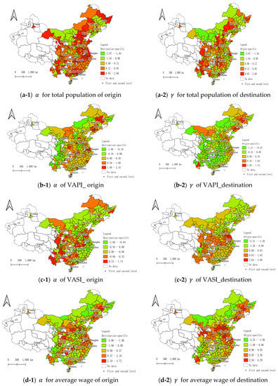
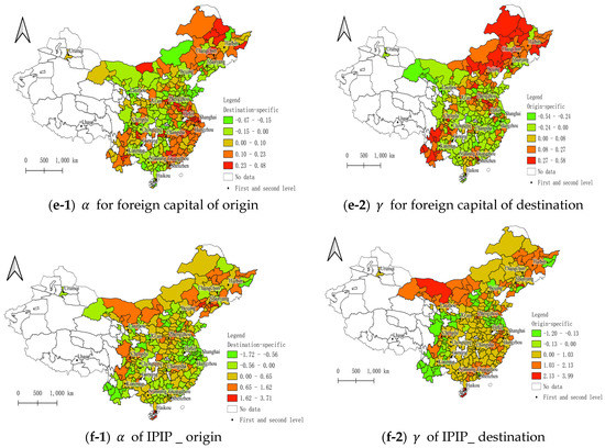
Figure 9.
Geographic distribution of estimation results of origin-specific and destination-specific interaction models.
From the regression results of the origin-specific and destination-specific interaction models, the following conclusions were drawn. (1) The estimated coefficients of total population in these two models differed from those of the global results. In the destination-specific model, the values of α for total population of origin in the first- and second-level cities (except for those in northeastern China) and in the cities surrounded by the four major city agglomerations were positive. In contrast, in a few cities in southwestern and central China and in most cities in northeastern and northern China, the estimated coefficients of total population were negative. In the origin-specific model, the γ values for total population of destination in the first- and second-level cities (except for the first- and second-level cities of northeastern China) and most cities of southwestern and central China were positive. However, in most cities in southeastern and southern China, the γ values for total population of destination were negative. The positive values of total population in most first- and second-level cities show that population growth promoted population inflow and outflow. However, most northeastern and northern cities and a few southwestern cities showed negative values of total population, demonstrating that these cities had a population loss. (2) In the destination-specific model, the α values for VAPI_origin were negative for western and northern cities. However, the α values for VAPI_origin were positive for northeastern and coastal cities (e.g., the Yangtze River Delta had high positive values). In the origin-specific model, the γ values of VAPI_destination were positive in some coastal, northern, and northeastern cities. However, these values were negative in central cities. Thus, the estimated coefficients of VAPI in some coastal cities and southwestern and northeastern cities of China were all positive. This illustrated that the population flow among these areas comprised primary-industry workers. (3) In the destination-specific model, the α values for VASI_origin were positive for most cities of southwestern China but negative for cities in northern and southeastern coastal cities. In the origin-specific model, the γ values of VASI_destination were positive in Chongqing and Jiangsu, Anhui, Hubei, Sichuan, Yunnan, and Shanxi. However, cities in northeastern China, the Yangtze River Delta, and the Pearl River Delta had negative values. Thus, the estimated coefficients of VASI were positive values in most cities in southwestern China, which indicated that these cities have gradually transformed into centers of secondary industry. In contrast, the negative estimated coefficients of VASI in most cities of northeastern China, the Yangtze River Delta, and the Pearl River Delta showed that tertiary industries dominate in these coastal developed cities and that few secondary-industry jobs are available. Conversely, although northeastern China is a long-established industrial area, it has a low attraction level to populations because of its severely decreased population. (4) In the destination-specific model, the α values for foreign capital of origin were positive for cities in northeastern China, southwestern China, and coastal areas, whereas in cities elsewhere, they were negative. In the origin-specific model, the γ values for foreign capital of destination were positive for cities in northeastern China, southwestern China, and the Pearl River Delta, whereas in cities elsewhere, they were negative. Thus, when cities in northeastern and southwestern China are a destination due to their having increased their attraction, this is as a result of the increased investment of foreign capital. For example, the Pearl River Delta was the earliest reformed and opened-up zone, and an enormous investment of foreign capital created a large number of jobs and attracted more workers to the area via population inflow. (5) In the southern and southeastern regions dominated by the Yangtze River Delta and Pearl River Delta, the α values for IPIP_origin were negative, and the γ values of IPIP_destination were positive. This is in line with the actual situation: these areas mostly contain high-development level coastal cities and are thus, major sites of population inflows.
5.2.3. Results of Origin-Focused and Destination-Focused Interaction Models
Although the origin-specific and destination-specific models consider spatial heterogeneity separately, they do not consider the effect of surrounding cities. Thus, the origin-focused and destination-focused models, which do consider the effect of surrounding cities, were used for this section of the work. The results are shown in Figure 10.
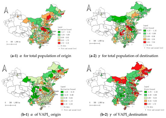
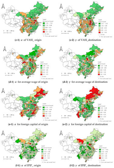
Figure 10.
Geographic distribution of estimation results for origin-focused and destination-focused interaction models.
The regression results of the origin-focused and destination-focused interaction models were largely the same as the results of the origin-specific and destination-specific models, but they differed in a few areas. These differences were as follows. (1) In Chongqing and some cities of Henan province, the α values for total population of origin in the destination-focused model were greater than those in the two specific models. Because Henan province and southwestern regions (where Chongqing is located) are the main areas of population outflow, this increase of α was in line with the actual situation. However, for some cities in the Yangtze River Delta, the α values for total population of origin were negative. This shows that these cities are becoming saturated with people. (2) The estimated γ values for VAPI_destination were negative in Henan and Anhui provinces, distinct from their positive values in the specific models. (3) The estimated α values for VASI_origin were positive in some cities of Anhui, Henan, and Hubei provinces, distinct from their negative values in the specific models. (4) The estimated α values for average wage of origin were negative in some cities of Shanxi province, distinct from their positive values in the specific models. Similarly, the estimated γ values for average wage of destination were positive in some cities of the Pearl River Delta, distinct from their negative values in the specific models. This is in line with the actual situation, as the increased income that is obtainable in these destination cities attracts more migrant workers, especially to large city agglomerations such as the Pearl River Delta. (5) The estimated α values for foreign capital of origin were negative in some cities of Anhui province, whereas the estimated γ values for foreign capital of destination were negative in some cities of Henan province and positive in Chongqing, all of which were opposite in sign to their values in the specific models. Thus, by increasing foreign investment in Chongqing, its population attractiveness has been improved. (6) The estimated α values for IPIP_origin were positive in some cities of Zhejiang province and Yunnan province, distinct from their negative values seen in the specific models. The estimated γ values for IPIP_destination were positive in some cities of Jiangsu province and negative in some cities of Anhui and Henan province, opposite from their signs in the specific models.
It can be seen that these differences were mainly concentrated in Henan, Anhui, Hubei, and Chongqing. This was attributable to the enormous variation in socioeconomic environments in these regions. The actual pattern in these regions could not be fitted by simple local-weighting approaches. The overall trend of parameter values in the results of focused and specific models was consistent. However, the results of focused models tended to be regionally consistent, e.g., the estimated parameters for the cities that are near the Pearl River Delta region were similar to the overall trend of the Pearl River Delta region. The results of specific models also tended to be discrete. For instance, in some individual cities in southwestern and northeastern regions, such as Chongqing and Shenyang, the estimated parameters differed depending on the surrounding cities or provinces. This clearly illustrated that the results of the two specific models were one-sided but that the results of the two focused models were regionally consistent.
5.2.4. Comparison of Spatial Interaction Models
We compare SWIMs with other spatial interaction models, as shown in Table 10. All of these models take the re-work dataset as input and obtain the fit results. All results satisfy the statistical hypothesis testing.
Table 10.
The fitting results of models.
As shown in Table 10, SWIMs of the origin-focused model and destination-focused model have the best goodness-of-fit, with the highest mean value of McFadden’s pseudo R2. This verifies that the SWIMs significantly outperform the other models, indicating that the weighted interactive model performed better by considering the local characteristics. The mapping of the McFadden pseudo R2 values in Figure 11 is an example of destination-based models, which illustrate that the use of these models is reasonable in more detail.
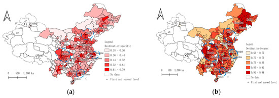
Figure 11.
The goodness-of-fits of destination-based models. (a) Pseudo R2 of destination-specific model, (b) Pseudo R2 of destination-focused model.
As shown in Figure 11, the Pseudo R2 values vary significantly across cities in different locations, indicating spatial heterogeneity in population flow. The Pseudo R2 values were higher in the city agglomerations with first- and second-level core cities, especially the four major city agglomerations that have been circled. This showed that cities in the same city agglomeration had similar patterns of population flow and that city agglomerations with a higher level of development had stronger radiation capacity (circled area in Figure 11b). In conclusion, the spatial distribution of the Pseudo R2 values in the results of these two models is consistent, which also validates the reasonableness of SWIMs.
In addition, as stated in the methodology, the gravity model and its relationships assume that greater flows will occur between larger and closer places than between smaller and more distant places, ceteris paribus. That is, the intensity of population flow decreases with increasing distance between two places and by the relatively steep distance-deterrence. Similarly, by mapping the value of distance-decay parameter β, the reasonableness of SWIMs can be illustrated in more detail, using the origin-based models in Figure 12 as an example.
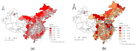
Figure 12.
The distance-decay parameter β of origin-based models. (a) β of Distance of origin-specific model, (b) β of Distance of origin-focused model.
The estimated value of the global distance-decay parameter β is −1.9758, as shown in Table 10, indicating the negative effects of distance on population flow, which is consistent with distance-decay. As shown in Figure 12, The distance-decay coefficient β in these two models has similar spatial distribution with the negative coefficient. β was the highest in the northern cities, followed by the southern coastal cities, and weakest in the central cities. Remarkably, the β of distance of some cities of Henan, Anhui, and Hubei provinces (among the six provinces in central China) was larger in the origin-focused models than it was in the origin-specific model (circled area in Figure 12b), because these areas are the buffer zone of the Yangtze River Delta and the Beijing–Tianjin–Hebei region, with a large population and congested traffic. Population flow within these areas is thus relatively more affected by distance factors. Therefore, on the one hand, by the fact that all β which are negative conformed to the distance-decay, the SWIMs are confirmed reasonable. On the other hand, the distinctive finding about Henan, Anhui, and Hubei provinces by distance factor is consistent with its by other factors mentioned above. By the discovery of consistency, it also showed that SWIMs are reasonable.
In summary, by comparing the goodness-of-fits of the models, SWIMs significantly outperform other spatial interaction models. At the same time, the reasonableness of SWIMs is verified based on spatial distributions of distance-decay and goodness-of-fit.
6. Discussion
6.1. Uncertainty Analysis
Although the above highly spatiotemporally detailed data provided new support for the study of population distribution and population flow, the intensity index of population migration was calculated based on the mobility information recorded from people’s mobile terminals. However, because not all users use AMAP applications, data deviation, data discontinuity, and data loss were inevitable. Moreover, privacy requirements prevented the accurate assessment of the purpose of the population flow; most is migrant worker flow, but there is some student and tourism flow. Furthermore, we only used an intensity index for population flow, rather than actual flow. All of these aspects mean that there is uncertainty in the data.
To obtain a more accurate population flow pattern and verify the results, we first divided the dataset into four subsets, according to the time node of the Spring Festival. Then, we analyzed the spatial and temporal trends of population mobility. The results of pattern exploration were consistent with previous findings in Yang et al. [13]. Thus, even though we used different platforms for dataset collection and the different methods of SNA to examine the same population flow during the Spring Festival of 2019, our results were consistent with those of Yang et al. [13]. This illustrated that our results were reasonable.
Furthermore, because population flow is restricted and influenced by many complex factors, selected socioeconomic factors devoid of multicollinearity problems were only explored with the help of spatial interaction models. We used a family of spatial interaction models to quantify the effect of socioeconomic factors on population flow. Some consensus conclusions were obtained, and these were in agreement. Although different results explained the improved performance of each model, the uncertainty of the results, due the limitations of the data, was not ignored.
To better consider the effect of surrounding cities in spatial interaction models, we applied a SWIM that incorporated the local weighting approach used in the GWR model to a spatial interaction model. Both the advantages and weaknesses of spatial-weighted regression models were inherited by this approach. The advantages were that the SWIM results were more regionally consistent than the one-sided results of specific models, which confirmed that the SWIM better considered the local characteristics of interactive processes. However, there were differences between the regression results of the SWIM and the specific models for the Henan, Anhui, Hubei, and Chongqing regions. Because these regions are large-scale population-focused and outflow areas, their population flow patterns are complex and multipatterned. Thus, their actual patterns are difficult to fit with simple local-weighting approaches. Indeed, the spatial-weighted regression models were only adapted to regions with similar patterns of population flow. Bandwidth is an important parameter that determines the range to which a city is affected. The optimal bandwidth results should be that the larger the urban agglomeration (B and C in Figure 13), the greater the bandwidth, and the greater its effects. However, in the northeastern regions (A in Figure 13), because of its sparse population, vast area, and lower level of sampling, the regression error was large, with a large bandwidth. Thus, when incorporating the local weighting approach of the GWR model into a SWIM, these ubiquitous problems must be noted. We believe that these problems will also be addressed in future work.
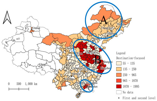
Figure 13.
Optimal bandwidth of destination-focused model.
6.2. Comparison with Related Research
Recent years have seen the emergence of a series of articles that attempted to comprehensively analyze the spatiotemporal patterns and influencing factors of population mobility. Compared with these related studies, this study has two innovations. First, we used population flow data, which are more highly spatiotemporally detailed. Second, we used advanced SNA methods and spatial interaction models to analyze spatiotemporal patterns and to quantify their effect. In particular, the SWIM is better at considering the local characteristics of an interactive process and was first implemented to study large-scale population flow. Compared with other spatial interaction models, the SWIM results are more detailed and meaningful.
7. Conclusions
In previous studies, the shortcomings of low spatiotemporally detailed data and the insufficient consideration of interactive differences in traditional spatial analysis models limited detailed study. In response to these problems, based on the population flow dataset collected from the AMAP Migration Map, we used a combination of SNA methods and spatial interaction models to explore the spatiotemporal patterns of population flow, and their determinants, during the Spring Festival in China. First, the SNA methods revealed that a hierarchy and a community structure existed in the spatiotemporal pattern of daily population flow. The hierarchical structure showed that the developmental level of a city was highly consistent with the intensity of its population flow and that the different network levels of population flow correlated with different developmental levels of cities. Thus, the nationwide network level was composed of the core cities (Beijing, Shanghai, Guangzhou, Chengdu, and Chongqing) of the four major city agglomerations, whereas the regional network level was composed of second-level cities (e.g., Xi’an, Kunming, and Guiyang). The community structure showed obvious correlations between city agglomerations and population flow in China, with the four major city agglomerations in China occupying core positions in these agglomerations. Most agglomerations were cross regional, and the population flow within the same community was relatively similar. In addition, most core cities of city agglomerations were the capital cities of their province.
Then, by using a family of spatial interaction models to reveal the effects of socioeconomic factors on re-work population flow, consistent conclusions were obtained. The results of these models showed that the population flow pattern was in line with the distance-decay effect, which was closely related to regional traffic development. Thus, population, as the determinant factor of the intensity of population flow, mainly flowed to the first- and second-level urban agglomerations, and population loss occurred in some cities of southwestern, northeastern, and northern China. The overall trend of value-added primary industry showed that most migrant workers were employed in primary industry. Moreover, primary-industry workers mainly flowed from the cities in southwestern and northwestern China to coastal areas. Furthermore, even though these cities were saturated with primary-industry workers, there was still a demand for secondary-industry workers; for example, in southwestern China, secondary industry was gradually increasing and attracting more workers. Income and foreign capital trends conformed to neoclassical theory, with an increase in income and foreign capital increasing the attractiveness of southwestern and northeastern China. In addition, the overall trend of pension insurance showed that attractiveness could be improved by improving the social security system.
Finally, these conclusions showed that there are obvious problems in China, such as unbalanced regional development, with population loss and unreasonable industrial allocation in some areas, which have led to differences in regional development conditions. Thus, our findings and conclusions may assist policymakers to control population loss, rationally allocate industrial structure, and balance development and will also promote progress in studies on population flow. In addition, these spatially weighted interactive models used in this study can be further applied to other large-scale population mobility issues or other spatial interaction issues, such as Thanksgiving in the United States. However, these spatially weighted interactive models suffer from some ubiquitous problems. Effectively selecting the optimal bandwidth and addressing the problem of under-sampling remain key challenges.
Author Contributions
Conceptualization, Tao Zhou; formal analysis, Tao Zhou and Bo Huang; funding acquisition, Bo Huang; methodology, Tao Zhou and Bo Huang; project administration, Cheng Xie and Qiang Gou; resources, Zhihui Huang; software, Bo Huang and Qiang Gou; supervision, Bo Huang; validation, Bo Huang; visualization, Cheng Xie and Qiang Gou; writing—original draft, Tao Zhou; writing—review & editing, Tao Zhou, Bo Huang, Xiaoqian Liu, Guangqin He and Cheng Xie. All authors have read and agreed to the published version of the manuscript.
Funding
This study is supported by the National Key R&D Program of China (2017YFB0503605).
Conflicts of Interest
The authors declare no conflict of interest.
References
- Wang, F.; Fan, W.; Lin, X.; Liu, J.; Ye, X. Does Population Mobility Contribute to Urbanization Convergence? Empirical Evidence from Three Major Urban Agglomerations in China. Sustainability 2020, 12, 458. [Google Scholar] [CrossRef]
- Yan, X.-Y.; Wang, W.-X.; Gao, Z.-Y.; Lai, Y.-C. Universal model of individual and population mobility on diverse spatial scales. Nat. Commun. 2017, 8, 1–9. [Google Scholar] [CrossRef] [PubMed]
- Soriano-Paños, D.; Arias-Castro, J.H.; Reyna-Lara, A.; Martínez, H.J.; Meloni, S.; Gómez-Gardenes, J. Vector-borne epidemics driven by human mobility. Phys. Rev. Res. 2020, 2, 013312. [Google Scholar] [CrossRef]
- Deville, P.; Song, C.; Eagle, N.; Blondel, V.D.; Barabási, A.-L.; Wang, D. Scaling identity connects human mobility and social interactions. Proc. Natl. Acad. Sci. USA 2016, 113, 7047–7052. [Google Scholar] [CrossRef] [PubMed]
- De Haas, H. Migration and development: A theoretical perspective. Int. Migr. Rev. 2010, 44, 227–264. [Google Scholar] [CrossRef] [PubMed]
- Rees, P.; Bell, M.; Kupiszewski, M.; Kupiszewska, D.; Ueffing, P.; Bernard, A.; Charles-Edwards, E.; Stillwell, J. The impact of internal migration on population redistribution: An international comparison. Popul. Space Place 2017, 23, e2036. [Google Scholar] [CrossRef]
- Wang, Y.; Deng, Y.; Ren, F.; Zhu, R.; Wang, P.; Du, T.; Du, Q. Analysing the spatial configuration of urban bus networks based on the geospatial network analysis method. Cities 2020, 96, 102406. [Google Scholar] [CrossRef]
- Zhu, R.; Lin, D.; Wang, Y.; Jendryke, M.; Xin, R.; Yang, J.; Guo, J.; Meng, L. Social Sensing of the Imbalance of Urban and Regional Development in China Through the Population Migration Network around Spring Festival. Sustainability 2020, 12, 3457. [Google Scholar] [CrossRef]
- Forbes. Chinese New Year: The World’s Largest Human Migration Is about to Begin; McCarthy, N., Ed.; Forbes: Jersey City, NJ, USA, 2018. [Google Scholar]
- Bogue, D.J. Internal migration. In The Study of Population; Hauser, P.M., Duncan, O.D., Eds.; University of Chicago Press: Chicago, IL, USA, 1959. [Google Scholar]
- Fan, C.C. Modeling interprovincial migration in China, 1985–2000. Eurasian Geogr. Econ. 2005, 46, 165–184. [Google Scholar] [CrossRef]
- Liu, Y.; Shen, J. Modelling Skilled and Less-Skilled Interregional Migrations in China, 2000–2005. Popul. Space Place 2017, 23, e2027. [Google Scholar] [CrossRef]
- Yang, Z.; Gao, W.; Zhao, X.; Hao, C.; Xie, X. Spatiotemporal Patterns of Population Mobility and its Determinants in Chinese Cities Based on Travel Big Data. Sustainability 2020, 12, 4012. [Google Scholar] [CrossRef]
- Cui, C.; Wu, X.; Liu, L.; Zhang, W. The spatial-temporal dynamics of daily intercity mobility in the Yangtze River Delta: An analysis using big data. Habitat Int. 2020, 102174. [Google Scholar] [CrossRef]
- Shang, J.; Li, P.; Li, L.; Chen, Y. The relationship between population growth and capital allocation in urbanization. Technol. Forecast. Soc. Chang. 2018, 135, 249–256. [Google Scholar] [CrossRef]
- Lai, J.B.; Pan, J.H. China’s City Network Structural Characteristics Based on Population Flow during Spring Festival Travel Rush: Empirical Analysis of “Tencent Migration” Big Data. J. Urban Plan. Dev. 2020, 146. [Google Scholar] [CrossRef]
- Pan, J.; Lai, J. Spatial pattern of population mobility among cities in China: Case study of the National Day plus Mid-Autumn Festival based on Tencent migration data. Cities 2019, 94, 55–69. [Google Scholar] [CrossRef]
- Xu, J.; Li, A.Y.; Li, D.; Liu, Y.; Du, Y.Y.; Pei, T.; Ma, T.; Zhou, C.H. Difference of urban development in China from the perspective of passenger transport around Spring Festival. Appl. Geogr. 2017, 87, 85–96. [Google Scholar] [CrossRef]
- Lancichinetti, A.; Fortunato, S. Community detection algorithms: A comparative analysis. Phys. Rev. E 2009, 80, 11. [Google Scholar] [CrossRef]
- Lewer, J.J.; Van den Berg, H. A gravity model of immigration. Econ. Lett. 2008, 99, 164–167. [Google Scholar] [CrossRef]
- Chen, R.; Wang, N.N.; Zhao, Y.; Zhou, Y.G. Complex network analysis of interprovincial mobile population based on improved gravity model. China Popul. Resour. Environ. 2014, 1. [Google Scholar]
- Zhang, X.N.; Wang, W.W.; Harris, R.; Leckie, G. Analysing inter-provincial urban migration flows in China: A new multilevel gravity model approach. Migr. Stud. 2018, 8, 19–42. [Google Scholar] [CrossRef]
- Kordi, M.; Fotheringham, A.S. Spatially weighted interaction models (SWIM). Ann. Am. Assoc. Geogr. 2016, 106, 990–1012. [Google Scholar] [CrossRef]
- Fotheringham, A.S.; O’Kelly, M.E. Spatial Interaction Models: Formulations and Applications; Kluwer Academic Publishers: Dordrecht, The Netherlands, 1989. [Google Scholar]
- Fotheringham, A.S.; Brunsdon, C.; Charlton, M. Geographically Weighted Regression: The Analysis of Spatially Varying Relationships; John Wiley & Sons: Hoboken, NJ, USA, 2003. [Google Scholar]
- Brunsdon, C.; Fotheringham, A.S.; Charlton, M.E. Geographically weighted regression: A method for exploring spatial nonstationarity. Geogr. Anal. 1996, 28, 281–298. [Google Scholar] [CrossRef]
- Zhu, X.; Wu, Y.; Chen, L.; Jing, N. Spatial Keyword Query of Region-Of-Interest Based on the Distributed Representation of Point-Of-Interest. ISPRS Int. J. Geo-Inf. 2019, 8, 287. [Google Scholar] [CrossRef]
- Qian, C.; Yi, C.; Cheng, C.; Pu, G.; Wei, X.; Zhang, H. GeoSOT-Based Spatiotemporal Index of Massive Trajectory Data. ISPRS Int. J. Geo-Inf. 2019, 8, 284. [Google Scholar] [CrossRef]
- Jinghu, P.; Jianbo, L. Research on spatial pattern of population mobility among cities: A case study of “Tencent Migration” big data in “National Day–Mid-Autumn Festival” vacation. Geogr. Res. 2019, 38, 1678–1693. [Google Scholar]
- Liu, W.; Hou, Q.; Xie, Z.; Mai, X. Urban Network and Regions in China: An Analysis of Daily Migration with Complex Networks Model. Sustainability 2020, 12, 3208. [Google Scholar] [CrossRef]
- Shen, J.; Liu, Y. Skilled and less-skilled interregional migration in China: A comparative analysis of spatial patterns and the decision to migrate in 2000–2005. Habitat Int. 2016, 57, 1–10. [Google Scholar] [CrossRef]
- Cao, Z.; Zheng, X.; Liu, Y.; Li, Y.; Chen, Y. Exploring the changing patterns of China’s migration and its determinants using census data of 2000 and 2010. Habitat Int. 2018, 82, 72–82. [Google Scholar] [CrossRef]
- Wang, Y.; Dong, L.; Liu, Y.; Huang, Z.; Liu, Y. Migration patterns in China extracted from mobile positioning data. Habitat Int. 2010, 86, 71–80. [Google Scholar] [CrossRef]
- Liu, T.; Qi, Y.; Cao, G. China’s floating population in the 21st century: Uneven landscape, influencing factors, and effects on urbanization. Acta Geogr. Sin. 2015, 70, 567–581. [Google Scholar] [CrossRef]
- Zhang, K.H.; Song, S. Rural–urban migration and urbanization in China: Evidence from time-series and cross-section analyses. China Econ. Rev. 2003, 14, 386–400. [Google Scholar] [CrossRef]
- Nordstrom, K.; Ekberg, K.; Hemmingsson, T.; Johansson, G. Sick leave and the impact of job-to-job mobility on the likelihood of remaining on the labour market—A longitudinal Swedish register study. BMC Public Health 2014, 14, 11. [Google Scholar] [CrossRef] [PubMed]
- Liu, Y.; Shen, J. Jobs or amenities? Location choices of interprovincial skilled migrants in China, 2000–2005. Popul. Space Place 2014, 20, 592–605. [Google Scholar] [CrossRef]
- Bei-Lei, Y.; Meng-Xian, W.; Fang-Du, Z. The impact of floating population’s social integration to their parents’ family supporting: Based on the empirical research of seven cities in 2013. Northwest Popul. J. 2017. [Google Scholar]
- Langville, A.N.; Meyer, C.D. A survey of eigenvector methods for web information retrieval. SIAM Rev. 2005, 47, 135–161. [Google Scholar] [CrossRef]
- Page, L.; Brin, S.; Motwani, R.; Winograd, T. The PageRank Citation Ranking: Bringing Order to the Web; InfoLab: Stanford, CA, USA, 1999. [Google Scholar]
- Parés, F.; Gasulla, D.G.; Vilalta, A.; Moreno, J.; Ayguadé, E.; Labarta, J.; Cortés, U.; Suzumura, T. Fluid communities: A competitive, scalable and diverse community detection algorithm. In International Conference on Complex Networks and Their Applications; Springer: Berlin/Heidelberg, Germany, 2017; pp. 229–240. [Google Scholar]
- Bickel, P.J.; Chen, A. A nonparametric view of network models and Newman–Girvan and other modularities. Proc. Natl. Acad. Sci. USA 2009, 106, 21068–21073. [Google Scholar] [CrossRef]
- Clauset, A.; Newman, M.E.; Moore, C. Finding community structure in very large networks. Phys. Rev. E 2004, 70, 066111. [Google Scholar] [CrossRef]
- Andersson, A.E.; Batten, D.F.; Johansson, B.; Nijkamp, P. Advances in Spatial Theory and Dynamics; North-Holland: Amsterdam, The Netherlands, 1989. [Google Scholar]
- Batten, D.F.; Boyce, D.E. Spatial interaction, transportation, and interregional commodity flow models. In Handbook of Regional and Urban Economics; Elsevier: Amsterdam, The Netherlands, 1987; pp. 357–406. [Google Scholar]
- Sen, A.; Sööt, S. Selected procedures for calibrating the generalized gravity model. In Papers of the Regional Science Association; Springer: Berlin/Heidelberg, Germany, 1981; pp. 165–176. [Google Scholar]
- Roy, J.R.; Thill, J.-C. Spatial interaction modelling. Papers Reg. Sci. 2003, 83, 339–361. [Google Scholar] [CrossRef]
- Hurvich, C.M.; Simonoff, J.S.; Tsai, C.L. Smoothing parameter selection in nonparametric regression using an improved Akaike information criterion. J. R. Stat. Soc. Ser. B (Stat. Methodol.) 1998, 60, 271–293. [Google Scholar] [CrossRef]
- Nakaya, T.; Fotheringham, A.S.; Brunsdon, C.; Charlton, M. Geographically weighted Poisson regression for disease association mapping. Stat. Med. 2005, 24, 2695–2717. [Google Scholar] [CrossRef]


Publisher’s Note: MDPI stays neutral with regard to jurisdictional claims in published maps and institutional affiliations. |
© 2020 by the authors. Licensee MDPI, Basel, Switzerland. This article is an open access article distributed under the terms and conditions of the Creative Commons Attribution (CC BY) license (http://creativecommons.org/licenses/by/4.0/).