Abstract
Social media data provide a great opportunity to investigate event flow in cities. Despite the advantages of social media data in these investigations, the data heterogeneity and big data size pose challenges to researchers seeking to identify useful information about events from the raw data. In addition, few studies have used social media posts to capture how events develop in space and time. This paper demonstrates an efficient approach based on machine learning and geovisualization to identify events and trace the development of these events in real-time. We conducted an empirical study to delineate the temporal and spatial evolution of a natural event (heavy precipitation) and a social event (Pope Francis’ visit to the US) in the New York City—Washington, DC regions. By investigating multiple features of Twitter data (message, author, time, and geographic location information), this paper demonstrates how voluntary local knowledge from tweets can be used to depict city dynamics, discover spatiotemporal characteristics of events, and convey real-time information.
1. Introduction
The rapid development of information and communications technology (ICT) has led to a proliferation of highly personalized mobility data collection extracted from social media posts. Social media services, especially micro-blogging platforms like Twitter, make it easy for people to share their thoughts about real-time events more spontaneously, providing information that can be extracted and used by researchers for a variety of purposes. From 2007 to 2013, the daily number of total tweets rocketed from five thousand to 500 million across the world [1]. The increasing amount of tweets and the abundant geographical content embedded in tweets have turned Twitter into a great resource for geographic mobility studies. Twitter data have been a great boon to geography researchers who struggle to collect geographic event information, which can be fleeting and dynamic.
Several key features of Twitter make it valuable in monitoring how events develop. First, the Twitter platform enables users to tweet about what is happening at any time and in any location. Second, users functioning as social sensors constantly report real-time or near real-time information to the public. The retweet feature (re-posting of someone else’s tweet) helps information spread wider and faster. Third, the geo-referenced tweets also provide explicit time-space descriptions of the events. Fourth, the large user base (both individuals and organizations) and broad geographic distribution of users offer a wide coverage of events across the world. These features have attracted a growing number of researchers who use Twitter data to investigate urban human activity and mobility patterns [2,3,4].
Despite the advantages of Twitter in geography research, the data heterogeneity and big data size make extracting useful information from Twitter data challenging [5]. Messages from users address a variety of topics and emotions, personal interests, and activities. Tweets also use abbreviations and unusual expressions or words. Extracting consistent information about events is difficult due to the abundant and varied content. Some major events can trigger a huge number of posts in a very short time period, making it difficult to efficiently handle the large data volume in time-sensitive applications. In recent years, many systems and algorithms have been developed to address these challenges [6], including approaches that analyze the spatial distribution of geotagged tweets, such as geospatial clustering or spatial-temporal scans [7]. Most prior studies focus on developing algorithms for event detection. Less attention has been given to analyzing the spatial-temporal evolution of the detected events. Finding patterns and sequences of events become essential in a state of continual event flux [8]. Questions, such as when and where events start to form and how the events dictate the evolution of tweets in space and time, are less documented.
In this paper, we present a systematic approach for harvesting, processing, and analyzing social media data in order to delineate the spatiotemporal evolution of events.
Our approach offers three unique contributions to the literature. First, this study uses real time streaming Twitter data. Unlike approaches such as spatial-temporal scans mainly used for batch processes, this study applies two moving windows to efficiently identify potential real time events in the study area. Second, the proposed approach also simultaneously discovers regional and local events based on features from multiple dimensions of tweets. Third, we also explore the spatial-temporal evolution and dynamics of natural and social events.
In this study, we develop an efficient approach based on machine learning and geovisualization by utilizing multiple dimensions of tweets (message, author, time, and location information), to identify the evolution of events, including planned events (e.g., festivals or sports) and incidental events (e.g., disasters or accidents). We trace the trajectory of the events through space and time. We demonstrate the method with two case studies, which analyze the temporal movement patterns of events in the New York City—Washington, DC area. By synthesizing multiple dimensions of Twitter data, this paper presents a method for creating spatiotemporal trajectories of events by mining voluntary data from social media platforms. It demonstrates a means of leveraging local knowledge to better depict city dynamics and discover spatiotemporal characteristics of events.
2. Related Work
Analyzing social media data to obtain geospatial information and event-related knowledge has received increasing attention [9,10,11]. Social media data present an unprecedented opportunity to study temporal dynamics in near real time and at multiple scales [8]. However, due to the noisy and complex nature of social media messages, extracting meaningful information is nontrivial. For instance, more than 200 million tweets were posted each day in 2011 [12]. Important urban information is often buried in a large pool of irrelevant data. Extracting meaningful information without smart text analytics and efficient strategies is practically impossible [12].
To facilitate such data extraction, recent studies have developed methods to capture the spatiotemporal patterns of human activities and urban events from Twitter data [6,13]. The event detection methods in these studies can be largely classified as targeted or general. Targeted event detection usually focuses on certain types of events based on a selection of words or hashtags, such as earthquakes [14], influenza epidemics [15], and sports games [16,17]. Tweets containing certain keywords or hashtags, such as “earthquake” or “NFL” can be used to accurately detect events related to the topic of interest. However, the collection of keywords may be subjective and exclude many other tweets related to the events. It may also require prior experience of the event to select the appropriate words to track [7]. Some recent studies have developed algorithms to deal with this issue. The TEDAS system was developed to detect crime and disaster-related events (CDE). This study manually set a collection of keywords related to CDE as seeds, and then applied an iteratively refined algorithm to extract new related keywords [4]. Laylavi et al. (2017) assessed the degree of relatedness of Twitter messages to a specific event of interest [18]. Wang et al. (2012) used a semantic role labeling approach to target crime-related tweets [19].
General event detection, in contrast, focuses on emerging topics that attract the attention of a large population (e.g., a hurricane or national festival) or local incidents that happen quickly in time and densely in space (e.g., traffic accidents or parade). A variety of methods have been used to detect these general events. Content-based detection methods use either document-pivot or term-pivot techniques [20,21]. Document-pivots usually apply clustering techniques to a document-term matrix to detect a topic in a large corpus. Term-pivot techniques work on n-grams features, aiming to detect representative terms for the event in question. Many data mining techniques have been used in these two approaches, including hierarchical clustering techniques based on pairwise distances [21], wavelet analysis of word frequencies to obtain features for each word [22], and locality sensitive hashing (LSH) to discover potential events [23]. For coordinate-based detection, spatial proximity has been widely used to prepare candidate tweets for local events [3,24]. DBSCAN has also been used to discover clusters with arbitrary shape [25]. The detected hot spots are likely to be associated with certain events.
The space-time scan statistic has been used to look for clusters of tweets across both space and time, regardless of tweet content. This method can detect various events, even within a relatively short time of data collection [7]. Temporal patterns of tweets can also be used to recognize events. Events usually exhibit a burst of features in Twitter streams, such as a sudden increase in specific keywords [20]. Lee used a sliding window technique to detect context changes and weighed message streams accordingly [26]. Boettcher and Lee used density-based clustering techniques on the tweets captured within a sliding time interval to detect potential events [24].
Many of the methods used to extract events, such as the space-time scan method, are based on location clustering techniques. These techniques are effective in the retrospective event detection (RED) context, because historical datasets usually contain rich point coordinates. However, we need approaches to tackle the challenge of new event detection (NED) from real time streams. Prior methods that tackle NED, such as hierarchical clustering, are computationally intensive and slow. Light-weight and efficient methods are needed to process the real time tweet data.
Many studies focus on event detection techniques, but fewer of them explore the spatial-temporal evolution of these events. Social media data may embed semantic meaning, background information, and sentiments in the content. This content is sometimes geo-tagged, either in the form of precise location from where these tweets were posted, or as toponyms of these locations [9]. Studies have reported that the percentage of precisely geo-tagged tweets may vary depending on the event, time, and location, ranging approximately from 0.5% to 5.0% of the total data corpus [9,27,28]. Although the overall percentage of geo-tagged tweets is not high, it is still possible to discern geo-tagged events from tweets at an aggregated level, especially at a regional scale. The semantic and locational information at regional scales provides a good opportunity to analyze the spatial-temporal evolution of events. The sentiments embedded in the tweets can also track public attitudes and emotions as the event develops. A few geographical studies have explored the progression of events by harvesting and analyzing geospatial information from social media content. These studies have explored the progression of natural disasters such as wildfires [29] and earthquakes [30]. The spatiotemporal analysis of Twitter content has also been used to track disease outbreaks and distribution [31,32].
This study aims to first develop an efficient approach to quickly scan multiple dimensions of tweets to capture real time and regional events, including planned (e.g., festivals or sports) and accidental (e.g., disasters or accidents) events and formulate thematic depictions of these events at their points of origin. Second, we trace the spatiotemporal trajectories of the formulated events to investigate spatiotemporal characteristics of those detected regional events and examine people’s reactions to these events.
3. Methods
Figure 1 shows the overall data process flow. Real-time Twitter data published via the streaming application-programming interface (API) are collected and parsed as MongoDB documents. Then, spatiotemporal information is read from the MongoDB document for the pattern recognition process. The computational model for pattern recognition was constructed in R language. Leaflet and R were used to visualize the results.
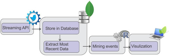
Figure 1.
The overall data process flow.
3.1. Data Collection
Data used in this study were piped into our system through Twitter streaming API in real-time. Twitter’s Geo API allows users to collect real-time tweet posts that are within a geographic area defined by a bounding box. In this study, we draw a bounding box that covers the metropolitan areas from New York City to Washington, DC. This area is not only one of the regions with the largest Twitter user population but also has cities with distinctive and prominent socioeconomic status. Washington, DC is the U.S. capital, and New York City is a world city with a decisive role in the world economy. The data are published using a standardized key-value structure. Much valuable geographic information can be extracted using this structure, such as user profiles and geographic locations of the tweets. Tweets collected from Geo API have at least one type of location data, such as location content, time zones, place names, and global positioning system (GPS) measurements. GPS information gives the most accurate point information of where a tweet was posted. The estimated median horizontal error range for GPS on smart phones is about 5–8.5 m [33]. As the majority of the tweets used GPS to denote their locations, we used only tweets with GPS information. In this study, the actual tweet message, the posting location and the time of the post were parsed. Each parsed tweet can be represented with the following expression: tw = (id; uid; twtxt; twtime; twloc) where id is tweet id, uid is user ID, twtxt is tweet message, twtime is timestamp, and twloc is geolocation. The information from each parsed tweet was saved as a MongoDB document. MongoDB supports text (non-spatial) queries as well as spatial queries. In order to improve MongoDB query performance, two indices have been created, one for the non-spatial id and another spatial index for the spatial twloc. For the spatial index, relative geographic relations of tweets can be created to indicate nearby tweets.
3.2. Data Pre-Processing
In this step, tweets were cleaned and filtered by removing non-English tweets, special characters, stop words, replacing capital letters with lower case, and tokenizing each tweet to individual words. Stop words were retrieved from SMART list in R tm package. We also detected other popular words in the study area based on historical tweets, such as “feel,” “watch,” and “friend” that are not included in stop-words packages. These words are less useful in the detection process and hence were removed from the set. We used the MC toolkit to tokenize a document into a vector space. MC toolkit is a C++ based program that creates vector-space models from text documents using multi-threaded implementation that can efficiently process very large document collections [34]. Suppose is the tweet data being processed, and is the content of . The result of the pre-preprocessing will split around whitespaces to generate a set of words . The phrase would be transformed to .
3.3. Layer Construction Module
Based on timestamps, tweets in a one-hour interval time window were first extracted and sent to a layer constructor. The constructor mapped each tweet t to its token number, user number, and coordinates number, namely a token-number tuple Pwn = (w, n), a token-user tuple Pwu = (w, u), and a token-coordinate tuple Pwc = (w, C), where n is the number of each token w, u is the number of users who mentioned the token w, and C is a list of coordinate pairs (lat, lon) in the study area associated with w. The constructor also computed each token’s frequency f(w) and the user frequency f(u) for each token w in the corpus. Tokens with a frequency smaller than three and tokens just mentioned by one user were excluded. These words account for a large proportion of total words but are very likely to be noise and are rarely associated with potential events. We thus discard these tokens and encapsulate the rest of the tokens to key-value hash tables. The keys are tokens, the values are token frequencies, user numbers, and lists of coordinates associated with each token. Results of this step include three hash sets with keys being the resultant tokens while values being the corresponding values from Pwu, Pwn, and Pwc for . A layer is a list made up of three hash sets.
In order to find the tokens that are potentially related to events, we used bursty word detection techniques. Bursty words are spikes in the frequency of tweets along the time spectrum. Event detection based on bursty words is similar to trend detection [24]. Instead of using traditional methods to detect bursty words, we designed two floating time-window pairs to better reveal events. The first window pair compares tokens that occurred in the most recent hour with the same tokens that occurred in the past four hours to . The second window pair compares tokens that occurred in the most recent hour with the same tokens that occurred at the same time a week ago . The system maintains two queues to store data in the two time window pairs. Each queue contains five components corresponding to five tables for each hour (Figure 2). When the system first launches, the ten components are calculated at once (represented by color blocks in Figure 2). In the following hours, only two components (the most recent hour and the same hour a week ago) are pushed respectively to the time window queues. The oldest components are popped from the queues. The rest are kept in the queue (represented by b/w color in Figure 2). The design of the moving window largely reduces the computational demand. Only two out of ten components need to be updated each hour. Tokens in the most recent hour are marked as the reference layer RL. Classification features are prepared based on the reference layer. The classification feature will be introduced in the following section.
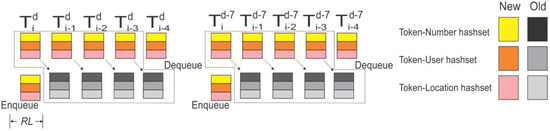
Figure 2.
Two queue structures to store three hash sets. Enqueue and dequeue happen at the beginning of each hour. Superscript represents day unit while subscript represents hour unit. RL represents the reference layer.
3.4. Feature Preparation Module
Once ten layers are constructed, classification features are prepared for identifying regional and local events. Tokens in the reference layer RL are used as observations. In other words, features will only be computed for tokens occurring in the RL. Tokens occurring in other layers but not in RL will not be computed.
Tokens related to events usually have four characteristics. First, words associated with major events tend to have a higher sudden increase in frequency. Second, tokens being tweeted by many people tend to indicate regional events. Third, regional events tend to be associated with a sudden increase in tokens from a wide geographic area. Fourth, tokens concentrated in a small area in a short time may imply local events.
To capture the first characteristic, we computed the frequency for each token ∈ in ten layers. To adjust the total tweet number at different times, we divided the token by the total tweet number in the time window to get the time adjusted token frequency.
There is a possibility that similar tweets are being tweeted by only one person or machine many times in a short time period. The contribution of keywords in such tweets should be discounted. For this reason, as with token frequency, we computed the user numbers for the ten layers as well. User numbers represent popularity of keywords among different users.
To account for the third characteristic, we computed the number of coordinates that are associated with token ∈ in ten layers. Tokens that are mentioned widely are more likely to be associated with a regional event.
Local events may contain densely reported messages. We used the DBSCAN technique to account for local clusters. DBSCAN is a clustering algorithm, which groups points that are closely located. DBSCAN requires two parameters: a minimum number of points and a maximum radius around one of its members (seed) to compute. Points within a radius of a given point, which satisfy the seed condition, are recursively selected as cluster members [35]. We used the “fpc” package in R to conduct the DBSCAN analysis. We scanned tokens with geographic coordinates and determined the two parameters by observing the size and average points for the local events. We used search radius eps = 0.0007 and minimum points MinPts = 3 as parameters in this study. The number of clusters and the total number of points in clusters were used as features.
Events usually occur when number of users, geographic coverage, and number of tokens have a sudden change. We calculated the ratios of features (i.e., features , , computed above) to capture the abrupt change. We computed two groups of ratios: (1) ratios of features between the most recent hour hi and the ones a week ago and (2) ratios of features between the past five hours hi–hi-4 and a week ago. A higher ratio represents a higher chance that the keyword is related to an event.
There are cases when a certain token w emerges in the reference layer (LR) but does not occur in the layer seven days earlier (Ld-7). To calculate the ratio for this case, we would have the “divide by zero” problem. Tokens in these cases can be further divided into scenarios S1 and S2. S1 contains random words (e.g., special words or misspelled words) in LR but not in Ld-7. These words have a low frequency in LR and are unlikely to be associated with events. S2 contains bursty words not occurring in Ld-7 but occurring frequently in LR. These words are very likely to be event-related words. We tested the 60th to 80th percentile and the results did not vary considerably. We thus used the 70th percentile of word frequency as the cutoff to distinguish these two scenarios. The words in S1 will be assigned a ratio of zero, and the ratio for words in S2 will be proportional to the word frequency in LR as shown in the following equation:
where R represents the ratio of word occurrence between the reference layer (LR) and the layer seven days ago (Ld-7), and calculates the frequency for the word w. The function quantile calculates the sample quantiles corresponding to the given probabilities as 0.7.
3.5. Classification Module
To prepare the training dataset, we manually sampled and coded 8167 tokens in consecutive days in August, 2015. Based on our pre-testing of different algorithms including kNN, SVM, Naive Bayes, and random forest (RF), we found the RF algorithm produced the highest accuracy in the classification performance. The RF classifier generates multiple decision trees in the training process to predict an outcome variable. To classify a new observation, random forest puts the variables into each of the trees in the forest. Each tree produces a classification result. The forest then chooses the classification with the most votes as the final classification. We used the “randomForest” package in R to conduct the RF analysis. In our model, we grew 200 trees to classify the input variables. The inputs of the classification module include 14 features: the time adjusted token frequency and the token frequency ratio in the time interval hi and hi to hi-4 respectively (4 features), the time adjusted user frequency and the user frequency ratio in the time interval hi and hi to hi-4 respectively (4 features), the time adjusted coordinate frequency and the coordinate frequency ratio in the time interval hi to hi-4 respectively (4 features), and the number of clusters and the total number of points in clusters (2 features). Outcomes of the model were dichotomous classes indicating whether a token belongs to an event class. The model also generates a probability score suggesting how likely the token is related to an event. We selected tokens with probability scores greater than 90% as event-related candidates.
Based on the trained model, each token in the hash set was labeled as event-related or not event-related. We define a potential event as a key-value tuple PE = (Ke, Ve) where Ke is a set of tokens being classified as event-related and V is a set of tweets. We used an association index between tokens in a term-document matrix to find tokens that are related to the same event in the set Ke. The association index indicates the correlation between a pair of terms among all tweets in the documents. A high association index represents a high probability that two words coexist in tweets. For instance, if we find tokens associated with the word “NYFW” (New York Fashion Week) with an association index greater than 0.4, we can detect the keyword “fashion.” All tweets associated with these keywords are put in the set Ve. Tweets that contain geographic coordinates are prepared and saved in a Shapefile for further pattern analysis.
3.6. Spatial-Temporal Evolution of Events
In the event analysis module, we mainly look at the temporal, spatial, and sentiment characteristics of an event. For temporal characteristics, we analyzed the time spectrum for a unique event and detect when this event starts, ends, or reaches prime time. For spatial characteristics, the spatial pattern evolution during the event was explored. Contour lines were created to display the density of tweets. Because city centers are usually the places most tweets concentrate, we used floating catchment area (FCA) to dampen the weight of tweets in densely distributed areas. Specifically, we drew a buffer with 0.05 degree around each related tweet to define a filtering window. The weight for each event-related tweet is inversely related to all tweets within the filtering window. We computed the kernel density based on the weight for each tweet across the study area. The kernel density spaces were investigated as time proceeded. For semantic characteristics, we analyzed popular expressions and created word clouds associated with each event. The SentiWordNet 3.0 English lexical resources were used to infer the sentiment of the event-related tweets. SentiWordNet is publicly available for supporting sentiment classification and opinion mining applications [36]. The background database WordNet includes a rich set of nouns, verbs, adjectives, and adverbs in different cognitive concepts and sentiment scores. We calculated sentiments of each tweet and aggregated them into an hourly window. Positive or negative scores represent positive or negative sentiments respectively. A score of zero means a neutral sentiment. Figure 3 summarizes the methods used in this study.
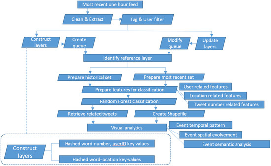
Figure 3.
Data analysis flow of this study.
4. Results
In the following sections, we select two events (natural & social) detected by the presented method to demonstrate the spatial, temporal, and sentiment dimensions of the events.
4.1. Heavy Precipitation
When we streamed tweets into the system and conducted event analysis around 9–10 September, we noticed a number of tweets mentioned rainy weather. After we collected data for the full month, we looked back and found a significant spike on 10 September in tweets about precipitation (Figure 4). We used the association function to look for keywords that were strongly associated with “rain.” Keywords including “wet,” “pour,” “flood,” and “umbrella” were detected.
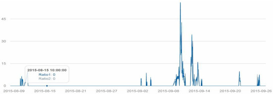
Figure 4.
Temporal spectrum of rain-related tweets between 8 August and 27 September. Ratio1 represents the one hour interval ratio while Ratio2 represents the five hour interval ratio.
We compared the spatial distributions of keywords about rain and the real-time cloud map in the study area. The kernel density estimation based on weights of rain-related tweets adjusted by the total number of tweets revealed a reasonable spatial pattern. We aggregated the tweets for four hours to increase the number of tweets with geographic coordinates to visualize. Although there was some discrepancy, the kernel density map of rain-related tweets conformed to the cloud map. For instance, at 5 a.m., the distribution and direction of rain-related tweets largely followed the cloud distribution. The areas with strong kernel density in Figure 5 largely correspond to the areas where heavy clouds were distributed.

Figure 5.
The spatial distributions of keywords about rain and the real-time cloud map in the study area.
Temporally, tweets about rain emerged at midnight on 10 September. Tweets about rain increased around 4 a.m. and reached their highest point around 8 a.m. The second peak occurred around 12 p.m.–1 p.m., and then the amount of rain-related tweets declined. Around 5–8 p.m., there was another small spike in rain-related tweets until the rain event ended at 8 a.m., 11 September. We also plotted the precipitation levels in three major cities (Philadelphia, Washington DC, and New York City) in the study area. We found that the intensity of rain-related tweets did not match well with the precipitation curve. More tweets were posted during times when more outdoor transportation was needed (morning peak transportation hours, noon, and afternoon peak hours). Another reason for this inconsistency might be that we only analyzed precipitation tweets from 3 cities, rather than choosing tweets from the whole study area (Figure 6).
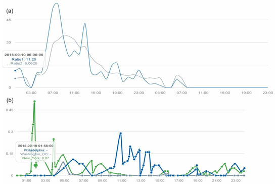
Figure 6.
(a) Temporal spectrum of rain-related tweets between 0–24 10 September. (b) The actual precipitation in inches in three cities on the same day.
Figure 7 shows the word cloud of the rain event. We computed sentiment scores for each rain-related tweet on 10 September. The score distribution was represented by the smoothed scatter plot. The purple line represents completely neutral sentiments while the green curve represents the median sentiment in each hour. Two blue curves wrapping around the green curve are the lower quartile and the higher quartile of sentiments. Overall, the median sentiment scores were slightly below zero, suggesting a mild negative sentiment. However, curves of lower and higher quartiles split on two sides of the neutral sentiment, suggesting mixed feelings about the rain. A closer look at the tweets reveals contradictory sentiments: “I love rain!!!!! I love rain boots!!!!!!!” vs. “This rain is just irritating.”
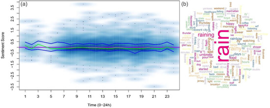
Figure 7.
(a) The scatter plot for the sentiment of tweets related to the rain event. The purple line represents neutral sentiments. Two blue curves wrapping around the green curve are lower quartile and higher quartile sentiments. The darker color represents higher tweet temporal density. (b) Word cloud of the rain event.
4.2. Pope Francis Visit
Pope Francis visited the United States for the first time from 22 September 2015 to 27 September 2015. This was an important social event that attracted many tweets. Pope Francis mainly traveled to three cities in the US: Washington, DC, New York City, and Philadelphia. We analyzed the tweet hotspots during his visit. Before the Pope visited the States, many tweets from both DC and Philadelphia showed that people were discussing the upcoming event. On 22–23 September, the tweets about the Pope were concentrated in DC where the Pope first visited. The tweet hotspot moved to New York on the 24th as the Pope flew there. The hotspot again migrated to Philadelphia on the 26th and peaked on the 27th when the Pope finished his visit to the US. The movement of the tweets largely conformed to the itinerary of the Pope (Figure 8).
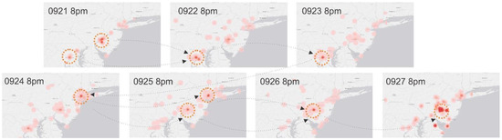
Figure 8.
Spatial movement of tweet hotspots during the time Pope Francis visit US.
Temporally, the Pope’s visit revealed an interesting pattern. The discussion about Pope Francis’s visit started on 21 September. There were two major peaks in tweets during the visit. The first major peak occurred on 22 September around 4 p.m., when the Pope arrived in D.C. The second one occurred on 24 September at 10 a.m. when the Pope gave a speech at the Senate and House of Representatives. During the six-day visit, discussion on Twitter about this event was more intensive in the morning but less intensive in the early afternoon. This fact also conforms to the Pope’s activity schedules. Discussion about the visits ended around 27 September at 11 p.m. (Figure 9).
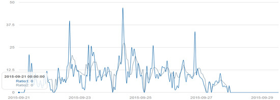
Figure 9.
Temporal spectrum of the Pope Visit related tweets between 21–29 September.
Figure 10 shows the major keywords from people’s tweets about the Pope’s visit. Sentiment analysis was also applied to this event. Unlike the rain event, the overall median sentiment scores were above zero while the lower quartile of the sentiment was close to zero. This distribution suggests an overall positive sentiment trend. This figure also reflects the duration of this event. After 28 September, the tweets about the event were much less frequent than on previous days.
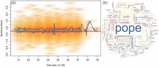
Figure 10.
(a) Scatter plot depicting the sentiments from the tweets about the Pope’s visit. The purple line represents a neutral sentiment; below the purple line represents negative sentiments and above the purple line represents positive sentiments. The two blue curves wrapping around the green curve are lower quartile and higher quartile. The darker color represent higher tweet temporal density. (b) Word cloud of keywords from tweets related to the Pope’s visit.
5. Discussion and Conclusions
Parkes and Thrift (1980) argue that urban life has a rhythmic pattern, formed by the spatial distribution of facilities and events and their temporal availability [37,38]. Now researchers can use Twitter data to make these invisible rhythmic patterns visible. The rhythmic pattern becomes even more visible when multiple days of data are displayed. We demonstrate how to use peaks of tweet data to identify significant events and start to identify the ebb and flow of urban life. Twitter data provide a unique window into unique urban spatial and temporal patterns.
In this study, we propose an innovative approach to identify event-related tweets by analyzing live-streaming Twitter data. This approach allows us to analyze streaming tweets, posted approximately one hour before collection. The prominent feature of this approach is that it does not assume any prior knowledge about events. Instead, it establishes knowledge about places as rhythmic profiles. No prior keywords were used to confine the domain of the events. This system only relies on streaming tweets. Other knowledge, such as news or GIS data, is not required to infer events. Hence, although the case study was conducted in the Washington, DC—New York City region, it can be applied to other geographic regions. By extracting training features from tweets (messages, users, timestamps, geo-coordinates), this system can discover the spatial-temporal development of regional events in near real time. Because we used sliding window and hash structures, they can quickly extract keywords associated with potential events. Keywords were used as the unit of the analysis. By applying association functions, we can find a set of keywords that are closely related to one event, and then extract the related tweets from the corpus.
We show how this approach can identify the spatial-temporal patterns of two events: a natural event and a social event. These two events have different temporal durations and geographic coverage. The rainy event spanned a day, while the Pope Visit event spanned a week. We were able to easily detect the start, end and peak of these events. When looking at the time-space patterns, the distribution of rain-related tweets generally conformed to the satellite cloud map while the tweets of the Pope related events reflected the itinerary of the visit. Additionally, the analysis also reflected people’s sentiments of the events. Such analysis enriches the geographic information by adding human perceptions to traditional GIS data.
By using features from both temporal and locational dimensions, the proposed method can capture both regional and local events. Numbers and ratios of users, tokens as well as the geographic coverage of tokens provide clues that the event is regional while the cluster size and numbers provide hints that the events are local. The analysis helps to discover geographic information at different scales. Figure 11 shows snapshots of the extracted regional and local events and their spatial distribution. For instance, we learned that 29 September was National Coffee Day. The tweets contained tokens “coffee” spread across the study area. Many people mentioned free coffee from Dunkin Donuts (e.g., “Nothing makes me happier than free coffee @DunkinDonuts #CoffeeDay”). We were also able to identify local events, such as the United States Conference on AIDS (USCA) on 10 September in Washington, DC, the US Open Tennis Championship (USOPEN) in Arthur Ashe Stadium on 2 September 2015, New York Fashion week on 10 September 2015, and the mixed martial arts event UFC 205 on 12 November 2016. Clustered and bursty tokens were observed for these local events.
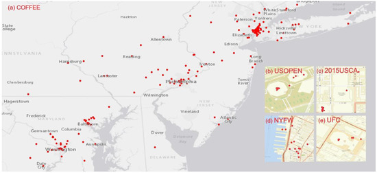
Figure 11.
Snapshots of the extracted regional and local event in the study area. (a) National Coffee Day. (b) US Open Tennis Championship (USOPEN) in Arthur Ashe Stadium. (c) United States Conference on AIDS (USCA) in Washington DC. (d) New York Fashion Week. (e) Martial arts event UFC 205.
This is an explorative study that extracted events from tweets published in a recent one-hour window. We acknowledge several limitations in this study. First, due to the low proportion of geo-tagged tweets, even though we can extract meaningful local events, only major local events can be revealed, especially in near real-time. Second, we used individual words as the analysis unit. Events described by phrases may not be captured as well using this approach. In future studies, we plan to compare the extracted events with information reported from traditional media and evaluate the relevancy of the events discovered from tweets. We also plan to extend this study in two ways. In this study, we only consider individual tokens, and the model was trained based on these tokens. We plan to incorporate a contiguous sequence of n items (n-grams) to better represent longer expressions. Second, the detected event-related keywords do not carry any additional attributes in the current approach. We do not know the relative importance of information extracted from tweets. We plan to discover the ranking for the importance of the detected events as well as the type of the event (e.g., sports) in our future work.
Acknowledgments
This study was supported by Georgia Southern University Seed Grant.
Author Contributions
Xiaolu Zhou and Chen Xu jointly collected and processed the data. Xiaolu Zhou wrote the draft manuscript. Chen Xu revised the manuscript.
Conflicts of Interest
The authors declare no conflict of interest.
References
- Statistics TU. Twitter Usage Statistics n.d. Available online: http://www.internetlivestats.com/twitter-statistics (accessed on 18 October 2015).
- Hasan, S.; Zhan, X.; Ukkusuri, S.V. (Eds.) Understanding urban human activity and mobility patterns using large-scale location-based data from online social media. In Proceedings of the 2nd ACM SIGKDD International Workshop on Urban Computing, Chicago, IL, USA, 11–14 August 2013; ACM: New York, NY, USA, 2013.
- Walther, M.; Kaisser, M. (Eds.) Geo-spatial event detection in the twitter stream. In Proceedings of the European Conference on Information Retrieval, Moscow, Russia, 24–27 March 2013; Springer: Berlin, Germany, 2013.
- Li, R.; Lei, K.H.; Khadiwala, R.; Chang, K.C.-C. (Eds.) Tedas: A twitter-based event detection and analysis system. In Proceedings of the 2012 IEEE 28th International Conference on Data Engineering, Arlington, VA, USA, 1–5 April 2012.
- Meladianos, P.; Nikolentzos, G.; Rousseau, F.; Stavrakas, Y.; Vazirgiannis, M. (Eds.) Degeneracy-based real-time sub-event detection in twitter stream. In Proceedings of the Ninth International AAAI Conference on Web and Social Media, Oxford, UK, 26–29 May 2015.
- Steiger, E.; Albuquerque, J.P.; Zipf, A. An advanced systematic literature review on spatiotemporal analyses of twitter data. Trans. GIS 2015, 19, 809–834. [Google Scholar] [CrossRef]
- Cheng, T.; Wicks, T. Event detection using Twitter: A spatio-temporal approach. PLoS ONE 2014, 9, e97807. [Google Scholar] [CrossRef] [PubMed]
- Peuquet, D.J.; Robinson, A.C.; Stehle, S.; Hardisty, F.A.; Luo, W. A method for discovery and analysis of temporal patterns in complex event data. Int. J. Geogr. Inf. Sci. 2015, 29, 1588–1611. [Google Scholar] [CrossRef]
- Panteras, G.; Wise, S.; Lu, X.; Croitoru, A.; Crooks, A.; Stefanidis, A. Triangulating social multimedia content for event localization using Flickr and Twitter. Trans. GIS 2015, 19, 694–715. [Google Scholar] [CrossRef]
- Cordeiro, M.; Gama, J. Online social networks event detection: A survey. In Solving Large Scale Learning Tasks Challenges and Algorithms; Springer: Berlin, Germany, 2016; pp. 1–41. [Google Scholar]
- Cherichi, S.; Faiz, R. Big Data Analysis for Event Detection in Microblogs. Recent Developments in Intelligent Information and Database Systems; Springer: Berlin, Germany, 2016; pp. 309–319. [Google Scholar]
- Chae, J.; Thom, D.; Bosch, H.; Jang, Y.; Maciejewski, R.; Ebert, D.S.; Ertl, T. (Eds.) Spatiotemporal social media analytics for abnormal event detection and examination using seasonal-trend decomposition. In Proceedings of the 2012 IEEE Conference on Visual Analytics Science and Technology (VAST), Seattle, WA, USA, 14–19 October 2012.
- Liu, Y.; Liu, X.; Gao, S.; Gong, L.; Kang, C.; Zhi, Y.; Chi, G.; Shi, L. Social sensing: A new approach to understanding our socioeconomic environments. Ann. Assoc. Am. Geogr. 2015, 105, 512–530. [Google Scholar] [CrossRef]
- Earle, P.S.; Bowden, D.C.; Guy, M. Twitter earthquake detection: Earthquake monitoring in a social world. Ann. Geophys. 2012, 54, 708–715. [Google Scholar]
- Aramaki, E.; Maskawa, S.; Morita, M. (Eds.) Twitter catches the flu: Detecting influenza epidemics using Twitter. In Proceedings of the Conference on Empirical Methods in Natural Language Processing, Edinburgh, UK, 27–31 July 2011; Association for Computational Linguistics: Stroudsburg, PA, USA, 2011.
- Zhao, S.; Zhong, L.; Wickramasuriya, J.; Vasudevan, V. Human as real-time sensors of social and physical events: A case study of twitter and sports games. arXiv, 2011; arXiv:11064300. [Google Scholar]
- Corney, D.; Martin, C.; Göker, A. (Eds.) Spot the ball: Detecting sports events on Twitter. In Proceedings of the European Conference on Information Retrieval, Amsterdam, the Netherlands, 13–17 April 2014; Springer: Berlin, Germany, 2014.
- Laylavi, F.; Rajabifard, A.; Kalantari, M. Event relatedness assessment of Twitter messages for emergency response. Inf. Process. Manag. 2017, 53, 266–280. [Google Scholar] [CrossRef]
- Wang, X.; Gerber, M.S.; Brown, D.E. (Eds.) Automatic crime prediction using events extracted from twitter posts. In Proceedings of the International Conference on Social Computing, Behavioral-Cultural Modeling, and Prediction, College Park, MD, USA, 3–5 April 2012; Springer: Berlin, Germany, 2012.
- Atefeh, F.; Khreich, W. A survey of techniques for event detection in twitter. Comput. Intell. 2015, 31, 132–164. [Google Scholar] [CrossRef]
- Ifrim, G.; Shi, B.; Brigadir, I. (Eds.) Event detection in twitter using aggressive filtering and hierarchical tweet clustering. In Proceedings of the Second Workshop on Social News on the Web (SNOW), Seoul, Korea, 8 April 2014; ACM: New York, NY, USA, 2014.
- Weng, J.; Lee, B.-S. Event Detection in Twitter. ICWSM 2011, 11, 401–408. [Google Scholar]
- Kaleel, S.B.; Abhari, A. Cluster-discovery of twitter messages for event detection and trending. J. Comput. Sci. 2015, 6, 47–57. [Google Scholar] [CrossRef]
- Boettcher, A.; Lee, D. (Eds.) Eventradar: A real-time local event detection scheme using twitter stream. In Proceedings of the 2012 IEEE International Conference on Green Computing and Communications (GreenCom), Besançon, France, 20–23 November 2012.
- Gomide, J.; Veloso, A.; Meira, W., Jr.; Almeida, V.; Benevenuto, F.; Ferraz, F.; Teixeira, M. (Eds.) Dengue surveillance based on a computational model of spatio-temporal locality of Twitter. In Proceedings of the 3rd International Web Science Conference, Koblenz, Germany, 14–17 June 2011; ACM: New York, NY, USA, 2011.
- Lee, C.-H. Mining spatio-temporal information on microblogging streams using a density-based online clustering method. Expert Syst. Appl. 2012, 39, 9623–9641. [Google Scholar] [CrossRef]
- Mahmud, J.; Nichols, J.; Drews, C. Where Is This Tweet From? Inferring Home Locations of Twitter Users. ICWSM 2012, 12, 511–514. [Google Scholar]
- Stefanidis, A.; Cotnoir, A.; Croitoru, A.; Crooks, A.; Rice, M.; Radzikowski, J. Demarcating new boundaries: Mapping virtual polycentric communities through social media content. Cartogr. Geogr. Inf. Sci. 2013, 40, 116–129. [Google Scholar] [CrossRef]
- De Longueville, B.; Smith, R.S.; Luraschi, G. (Eds.) Omg, from here, i can see the flames!: A use case of mining location based social networks to acquire spatio-temporal data on forest fires. In Proceedings of the 2009 International Workshop on Location Based Social Networks, Seattle, WA, USA, 3 November 2009; ACM: New York, NY, USA, 2009.
- Crooks, A.; Croitoru, A.; Stefanidis, A.; Radzikowski, J. # Earthquake: Twitter as a distributed sensor system. Trans. GIS 2013, 17, 124–147. [Google Scholar]
- Allen, C.; Tsou, M.-H.; Aslam, A.; Nagel, A.; Gawron, J.-M. Applying GIS and Machine Learning Methods to Twitter Data for Multiscale Surveillance of Influenza. PLoS ONE 2016, 11, e0157734. [Google Scholar] [CrossRef] [PubMed]
- Signorini, A.; Segre, A.M.; Polgreen, P.M. The use of Twitter to track levels of disease activity and public concern in the US during the influenza A H1N1 pandemic. PLoS ONE 2011, 6, e19467. [Google Scholar] [CrossRef] [PubMed]
- Zandbergen, P.A.; Barbeau, S.J. Positional accuracy of assisted gps data from high-sensitivity gps-enabled mobile phones. J. Navig. 2011, 64, 381–399. [Google Scholar] [CrossRef]
- Dhillon, I.S.; Modha, D.S. Concept decompositions for large sparse text data using clustering. Mach. Learn. 2001, 42, 143–175. [Google Scholar] [CrossRef]
- Ester, M.; Kriegel, H.-P.; Sander, J.; Xu, X. (Eds.) A Density-Based Algorithm for Discovering Clusters in Large Spatial Databases with Noise; Kdd: Portland, OR, USA, 1996.
- Baccianella, S.; Esuli, A.; Sebastiani, F. SentiWordNet 3.0: An Enhanced Lexical Resource for Sentiment Analysis and Opinion Mining. Available online: http://nmis.isti.cnr.it/sebastiani/Publications/LREC10.pdf (accessed on 17 March 2017).
- Parkes, D.; Thrift, N.J. Times, Spaces, and Places: A Chronogeographic Perspective; John Wiley: New York, NY, USA, 1980. [Google Scholar]
- Lefebvre, H. The Urban Revolution; University of Minnesota Press: Minneapolis, MN, USA, 2003. [Google Scholar]
© 2017 by the authors. Licensee MDPI, Basel, Switzerland. This article is an open access article distributed under the terms and conditions of the Creative Commons Attribution (CC BY) license ( http://creativecommons.org/licenses/by/4.0/).