
Extraction and Reconstruction of Zebra Crossings from High Resolution Aerial Images


Abstract
:1. Introduction
2. Methodology
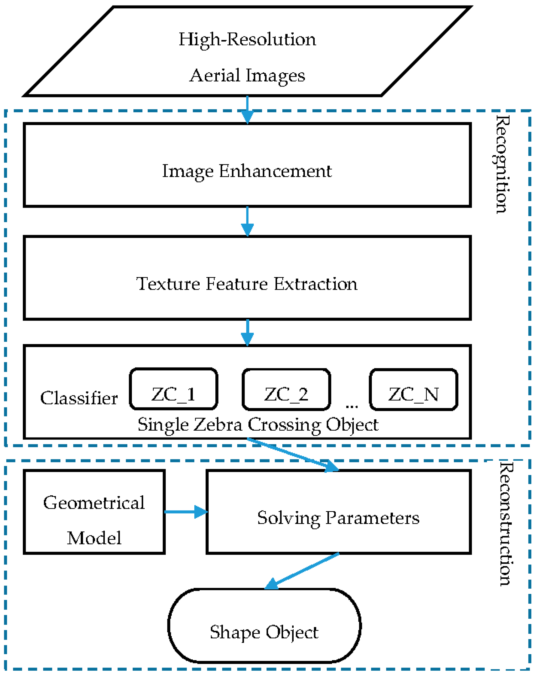
2.1. Method Overview
2.2. Zebra Crossing Extraction
2.2.1. Features Definition
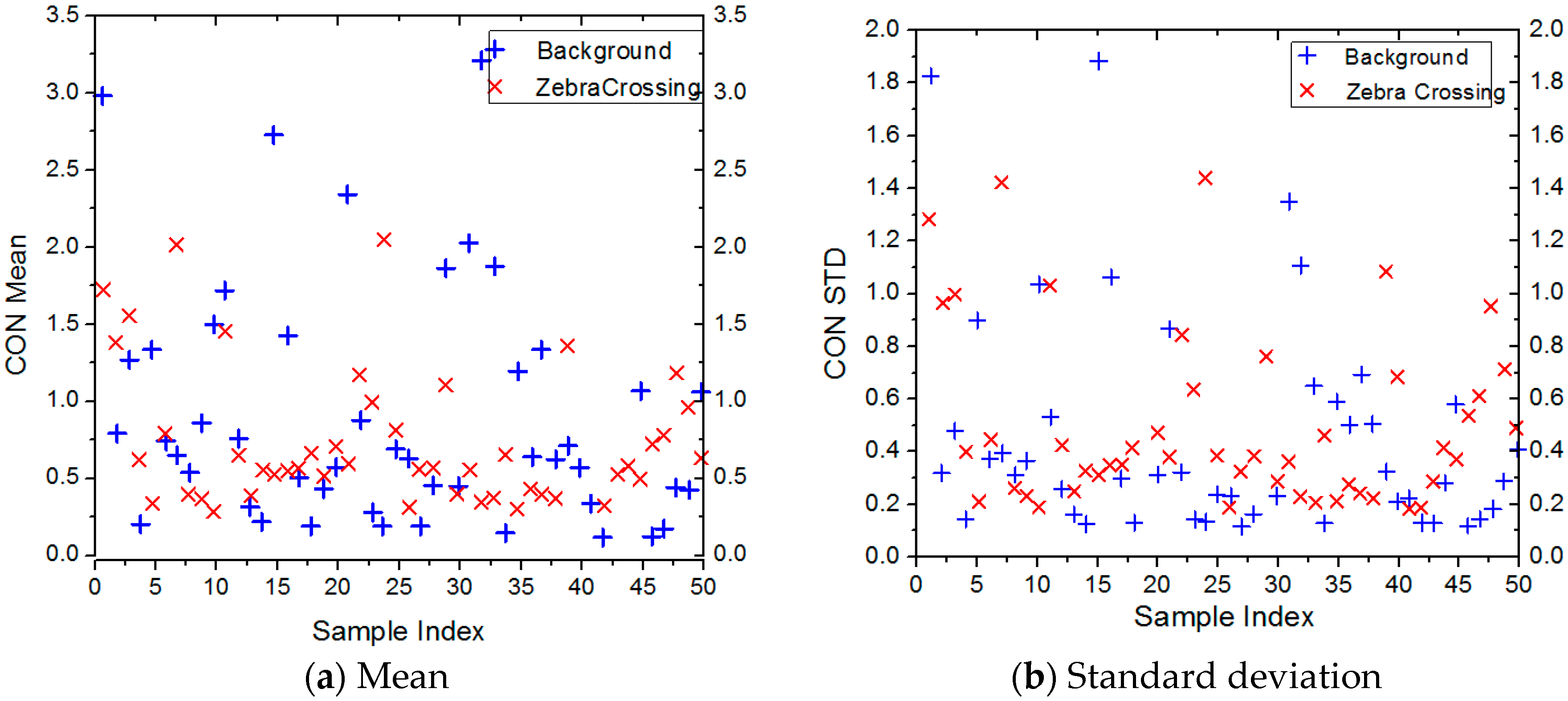
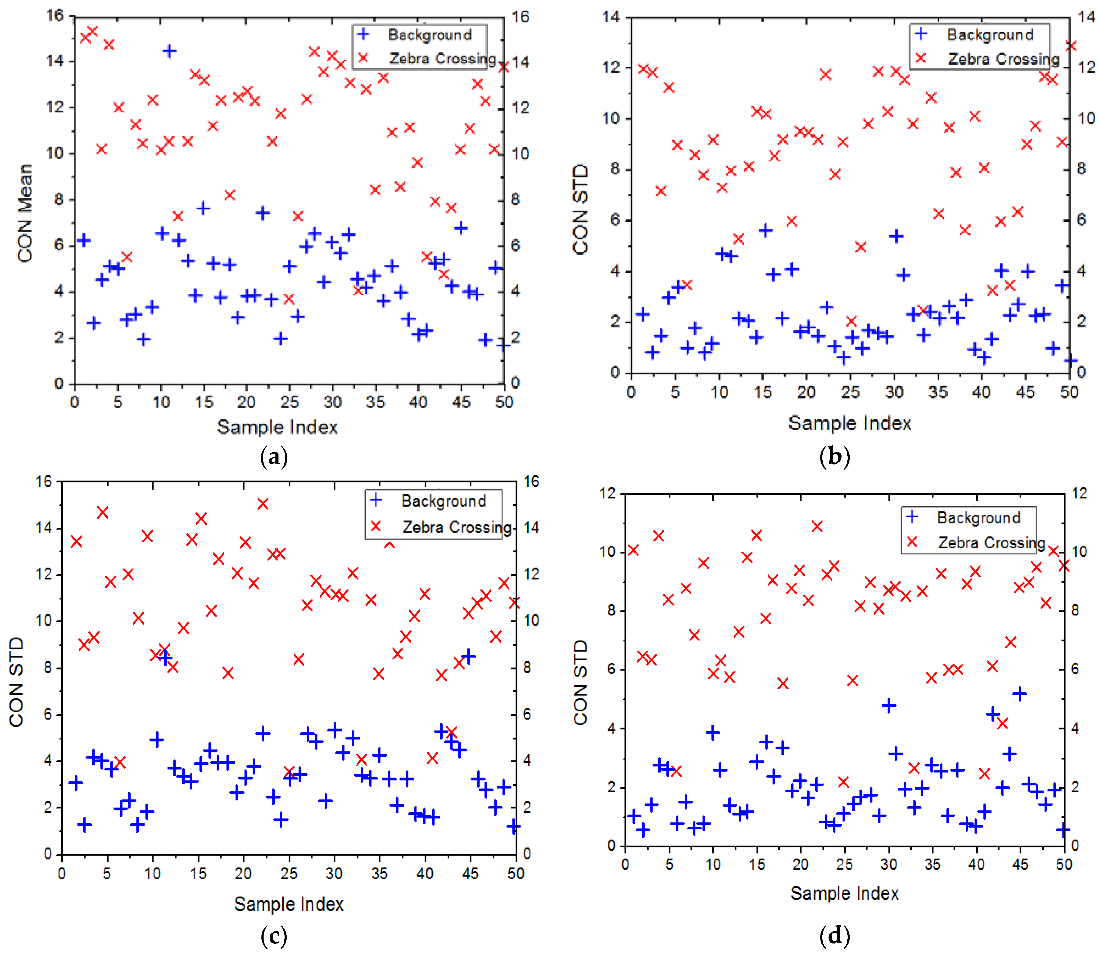
GLCM Features
- (1)
- Angular Second Moment:where represents the number of distinct gray levels in the images and is the (i, j)th entry in the GLCM. This statistic is also called Uniformity, which measures the textural uniformity and disorders.
- (2)
- Correlation:where , , and are the means and standard deviations of summarized rows and columns. The correlation feature measures gray-tone linear dependencies in the image.
- (3)
- Contrast:
- (4)
- Homogeneity:
- (5)
- Entropy:
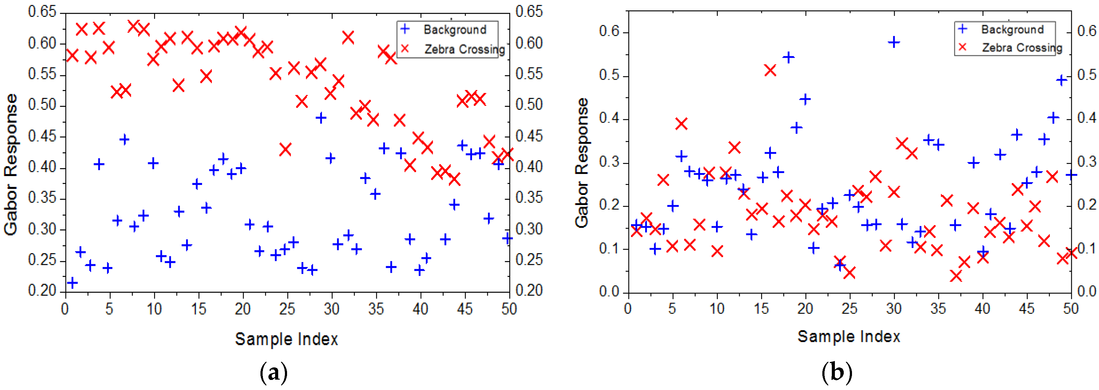
2D Gabor Feature
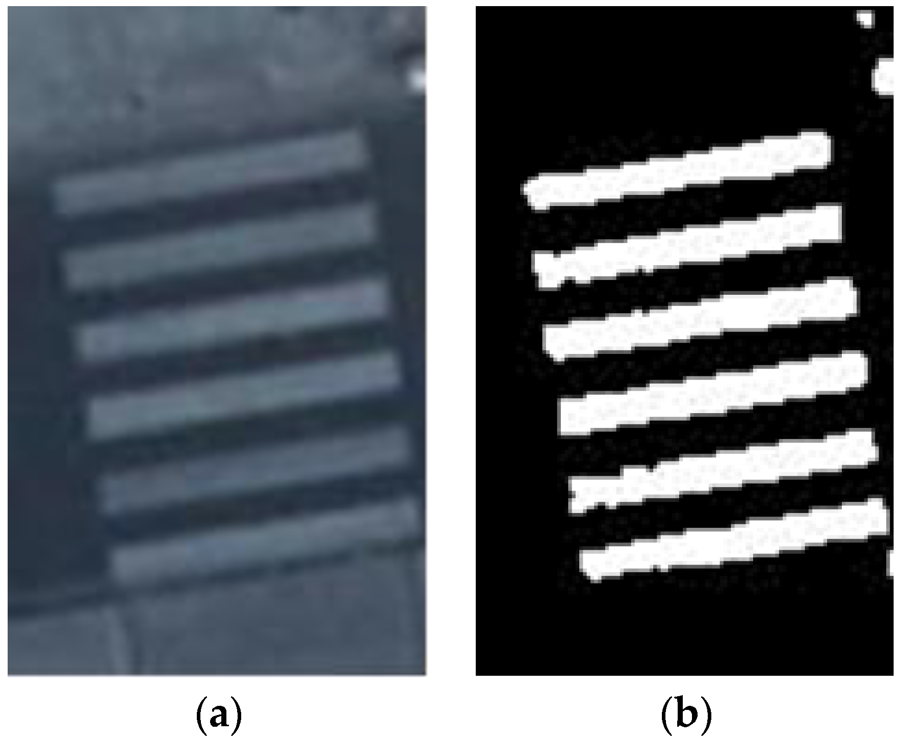
2.2.2. Extraction of Zebra Crossings
Principle of JointBoost
Extraction by JointBoost
2.3. Zebra Crossing Reconstruction
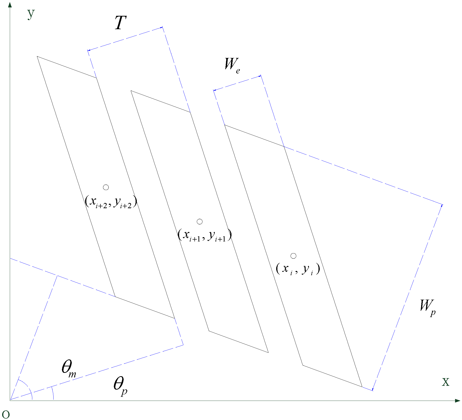
2.3.1. Geometrical Model
- (1)
- : the angle of the zebra crossings normal to their principle direction.
- (2)
- : the angle of the stripes normal to their principle direction.
- (3)
- : the length of the stripe.
- (4)
- : the width of the stripe.
- (5)
- : the interval of two neighbor stripes.
- (6)
- : the set of center points of the stripes.
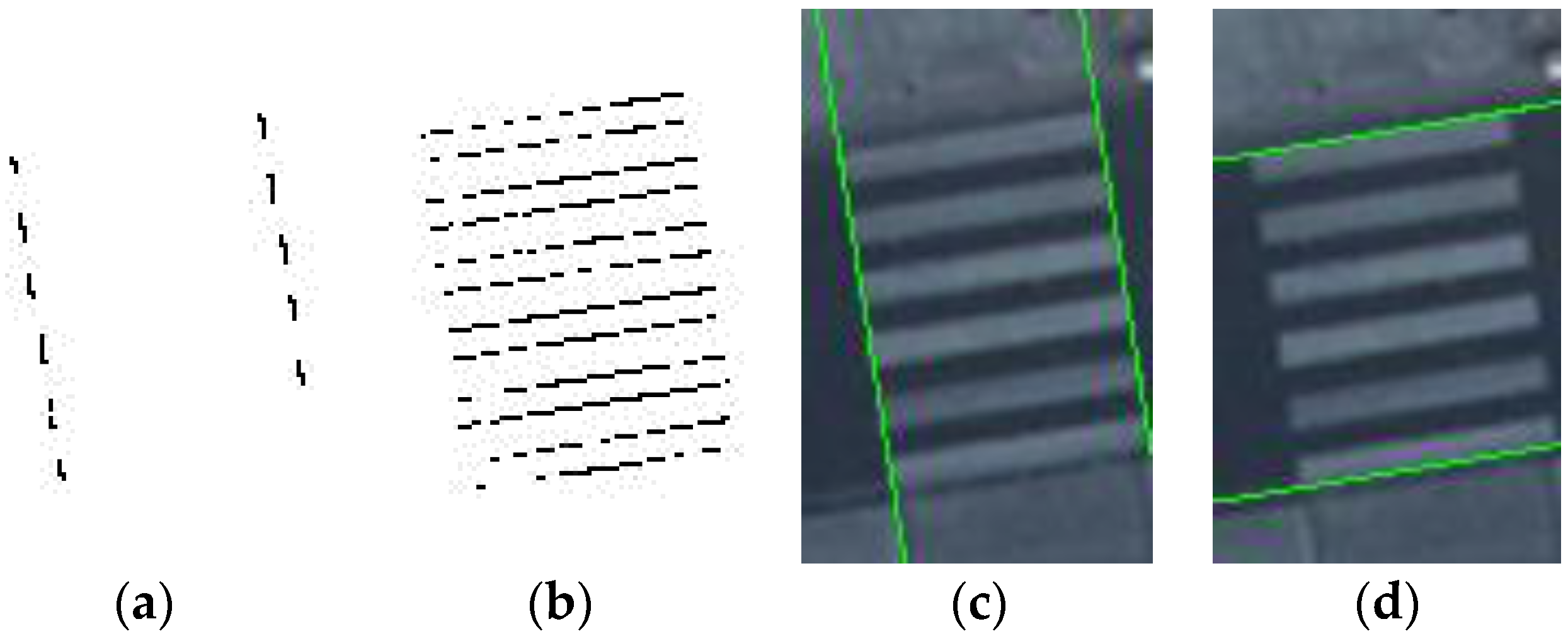
2.3.2. Solve the Parameters
- Step I:
- The Scope
- Step II:
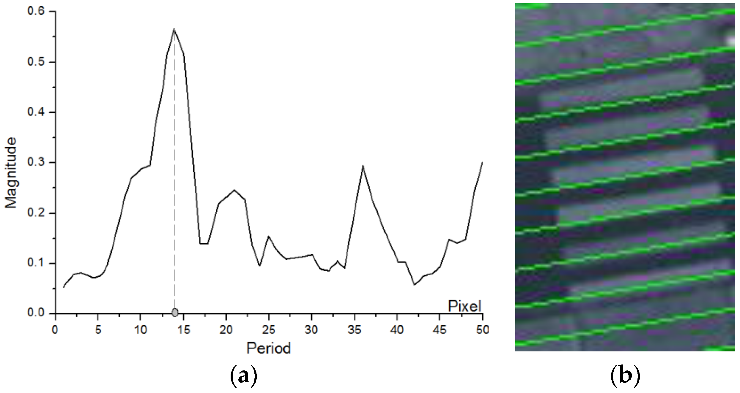
- The Spatial Repetitive Period
- Step III:
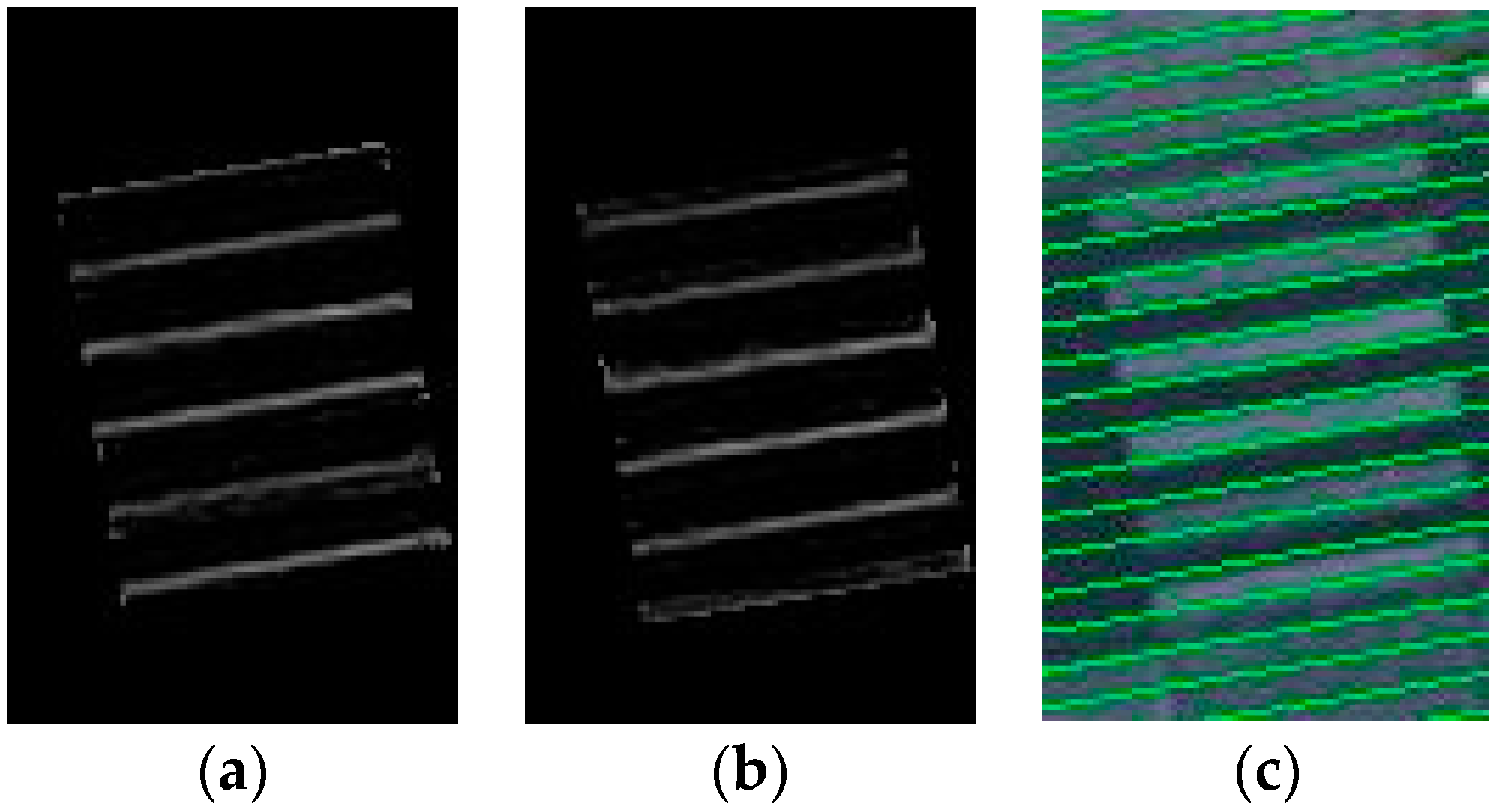
- The Width and Centers
- Step IV:
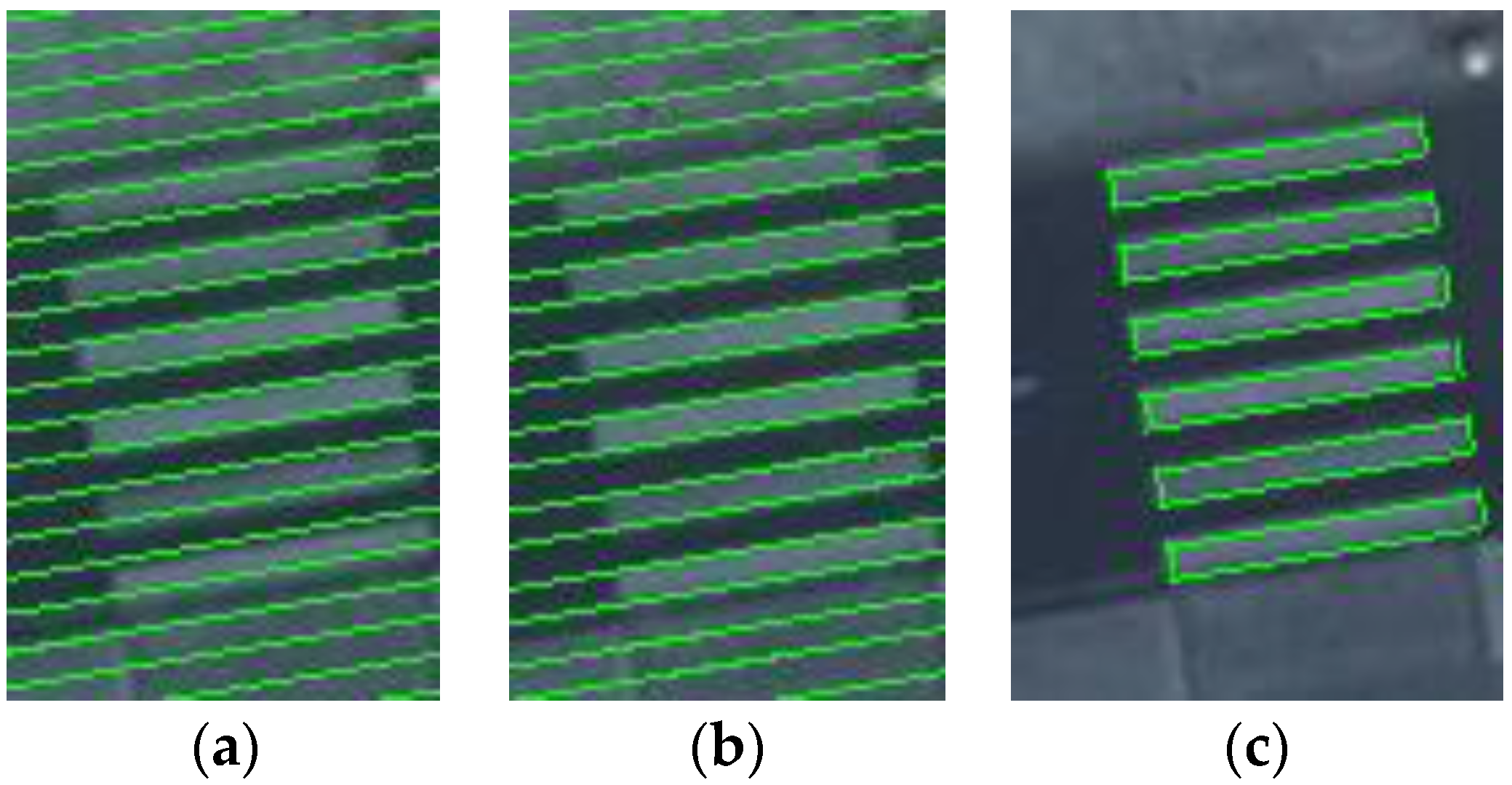
- Global Optimization
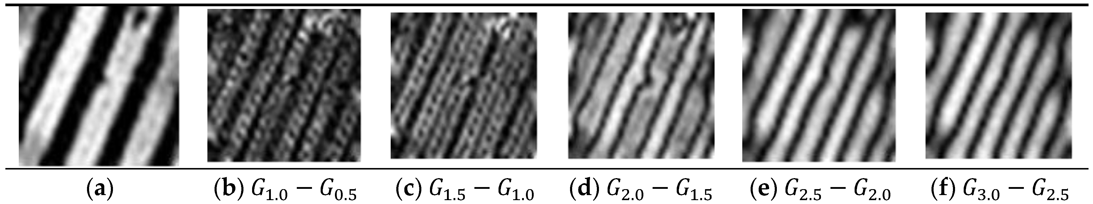
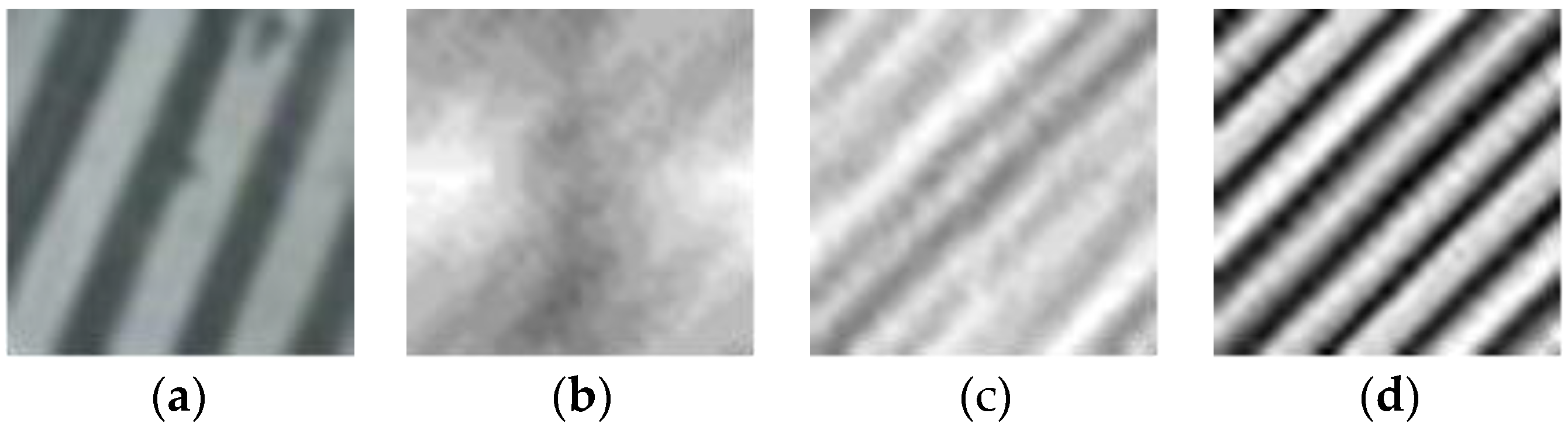
2.3.3. Repair Discontinuities
- Rule 1: The distance of two zebra crossing parts should be smaller than a threshold.
- Rule 2: When fitting the center points to a line, the residual should be smaller than a threshold.
- Rule 3: When selecting two stripe’s center points and , the distance between and should be integral multiples of the repetition period.
3. Experiments Section
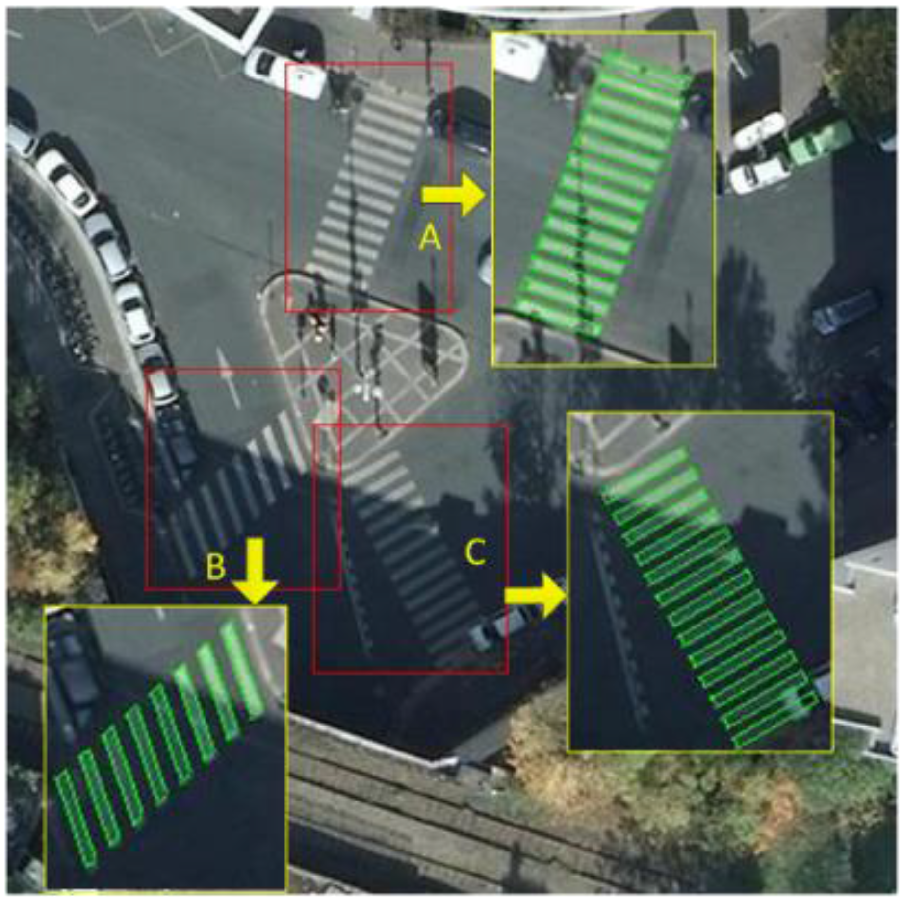
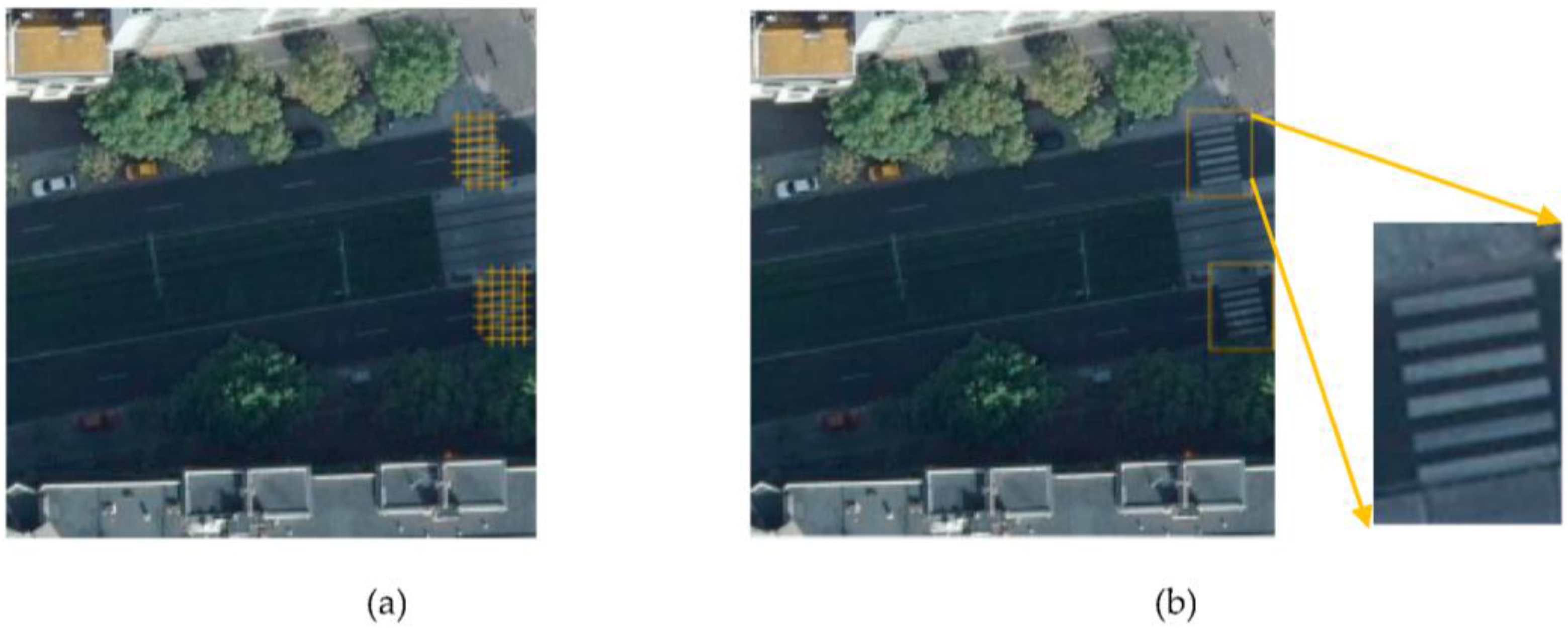
3.1. Zebra Crossing Extraction
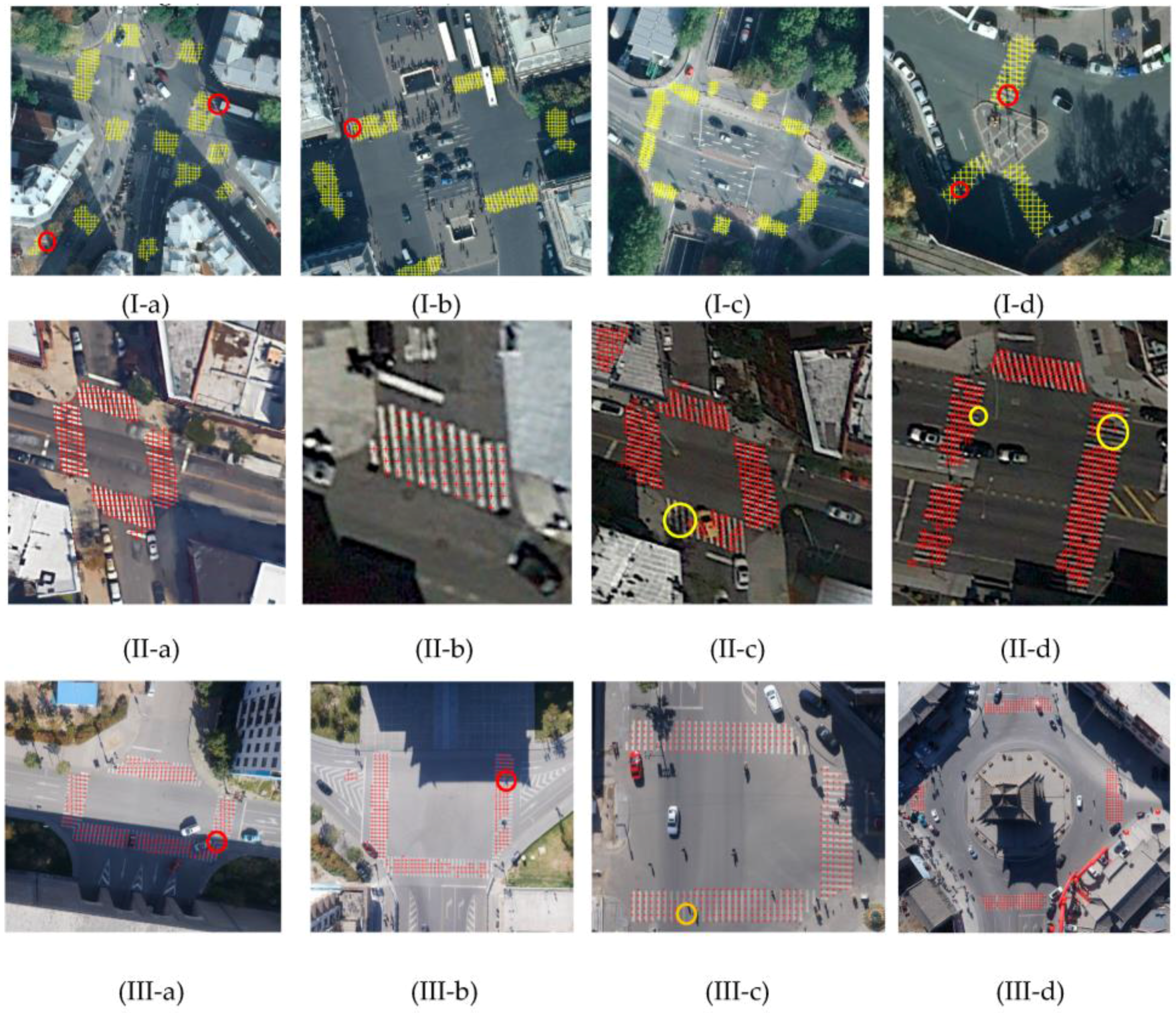
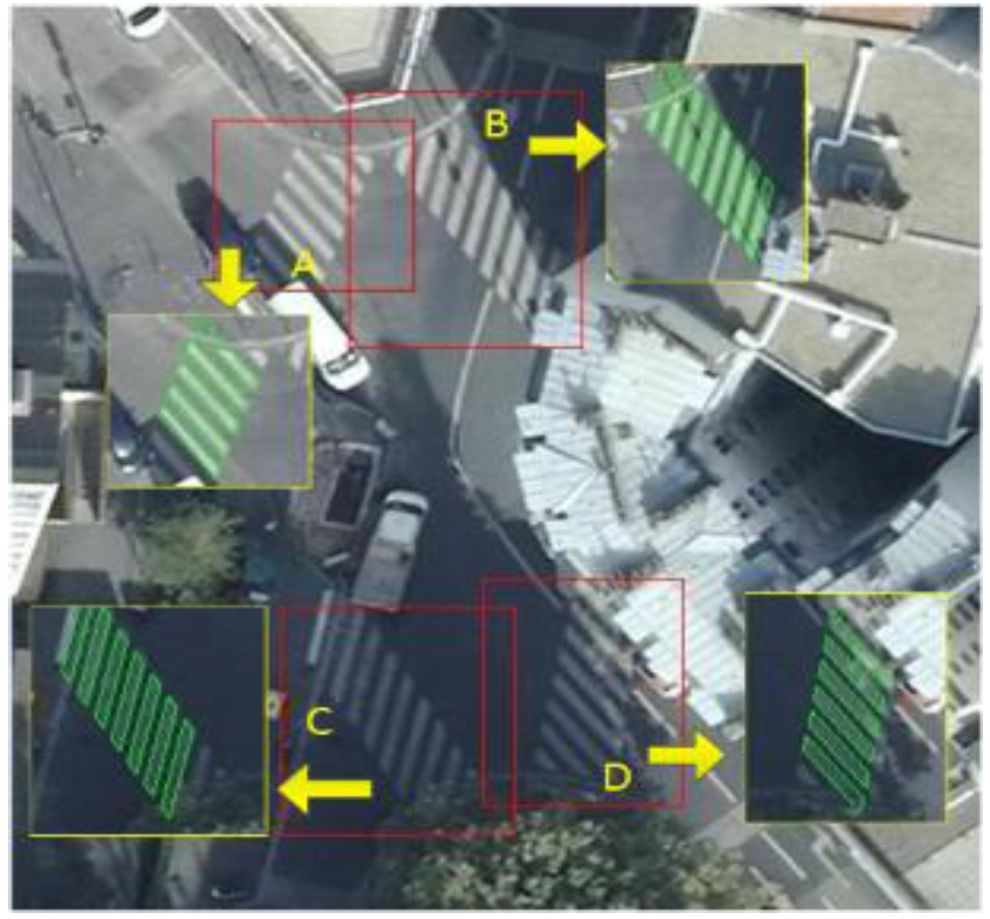
3.1.1. Experiment I: Zebra Crossing Detection
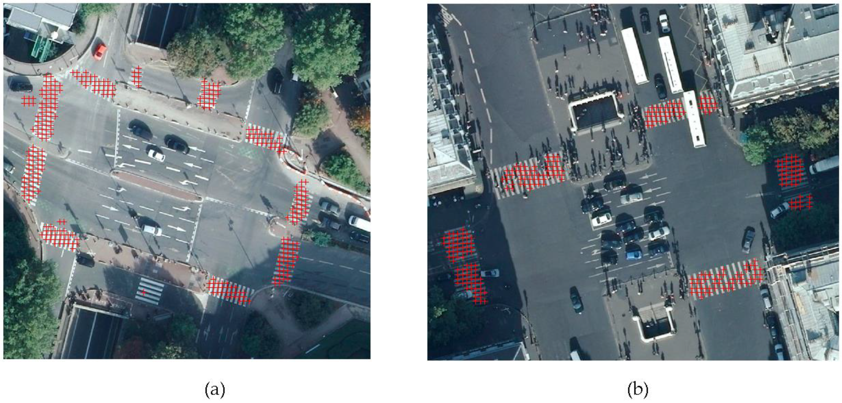
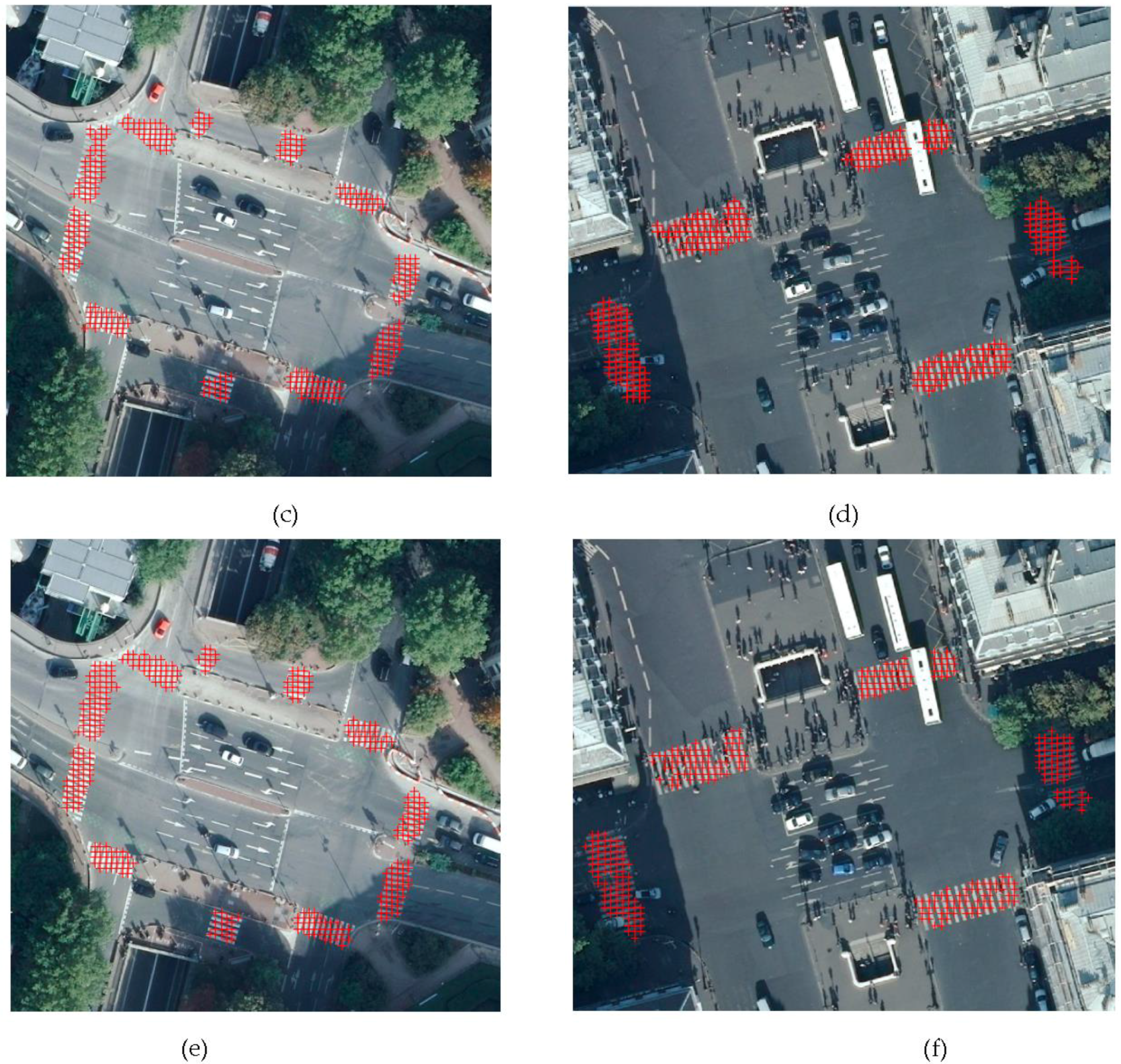
3.1.2. Effectiveness of Features
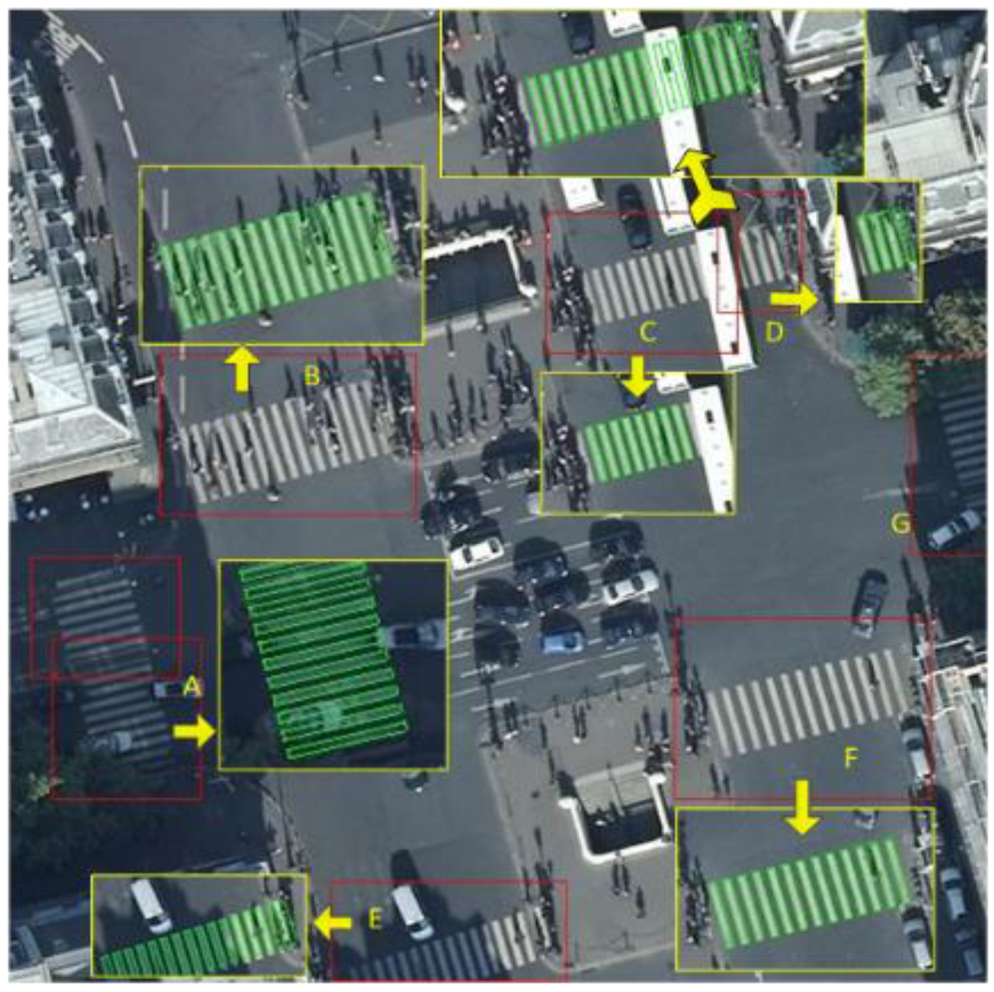
3.2. Geometric Shape Reconstruction
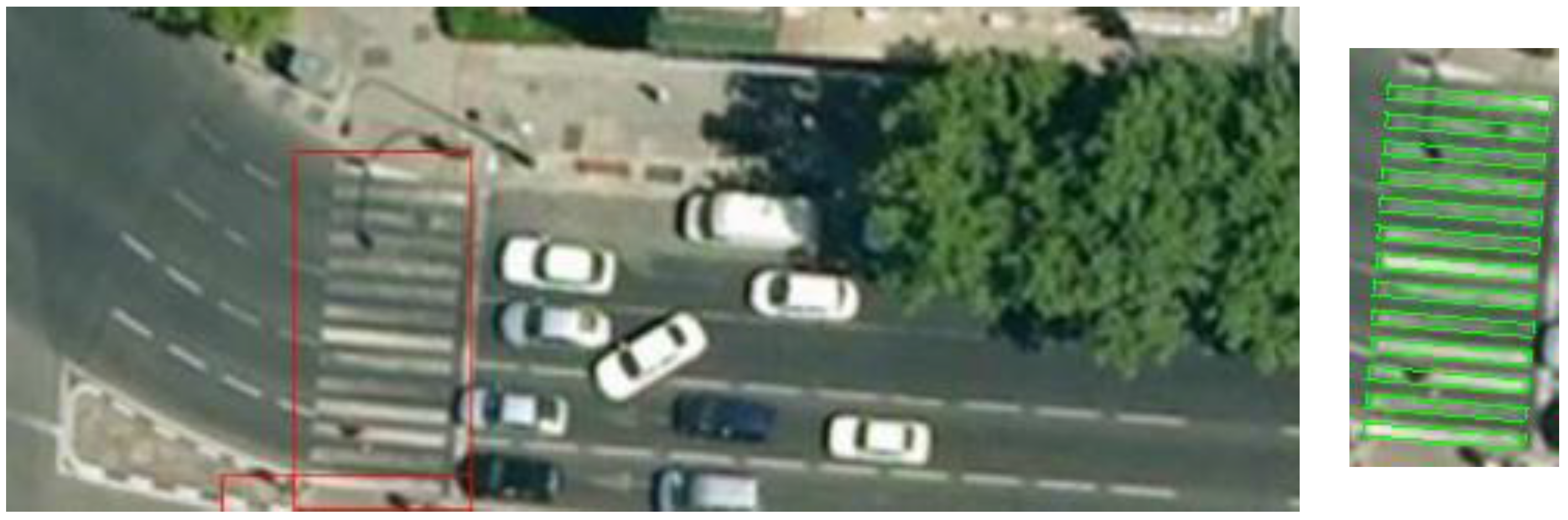
3.2.1. Zebra Crossing Covered by Objects
3.2.2. Rhomboid Zebra Crossing
3.2.3. Zebra Crossing with Shadow
3.2.4. Blurred Zebra Crossing
4. Discussion and Conclusions
Acknowledgments
Author Contributions
Conflicts of Interest
References
- Shi, W.; Miao, Z.; Debayle, J. An integrated method for urban main-road centerline extraction from optical remotely sensed imagery. IEEE Trans. Geosci. Remote Sens. 2014, 52, 3359–3372. [Google Scholar] [CrossRef]
- Hinz, S.; Baumgartner, A. Automatic extraction of urban road networks from multi-view aerial imagery. ISPRS J. Photogramm. Remote Sens. 2003, 58, 83–98. [Google Scholar] [CrossRef]
- Thomas, G.; Donikian, S. Virtual humans animation in informed urban environments. In Proceedings of the Computer Animation 2000, Philadelphia, PA, USA, 3–5 May 2000; pp. 112–119.
- Narzt, W.; Pomberger, G.; Ferscha, A.; Kolb, D.; Müller, R.; Wieghardt, J.; Hörtner, H.; Lindinger, C. Augmented reality navigation systems. Univ. Access Inf. Soc. 2006, 4, 177–187. [Google Scholar] [CrossRef]
- Rebut, J.; Bensrhair, A.; Toulminet, G. Image segmentation and pattern recognition for road marking analysis. IEEE Int. Symp. Ind. Electron. 2004, 1, 727–732. [Google Scholar]
- Royer, E.; Lhuillier, M.; Dhome, M.; Lavest, J.-M. Localisation par vision monoculaire pour la navigation autonome d’un robot mobile. In Proceedings of the Congrès Francophone AFRIF-AFIA de Reconnaissance des Formes et D’intelligence Artificielle, Tours, Frence, 25–27 January 2006.
- Sichelschmidt, S.; Haselhoff, A.; Kummert, A.; Roehder, M.; Elias, B.; Berns, K. Pedestrian crossing detecting as a part of an urban pedestrian safety system. In Proceedings of the 2010 IEEE on Intelligent Vehicles Symposium (IV), San Diego, CA, USA, 21–24 June 2010; pp. 840–844.
- Benz, U.C.; Hofmann, P.; Willhauck, G.; Lingenfelder, I.; Heynen, M. Multi-resolution, object-oriented fuzzy analysis of remote sensing data for gis-ready information. ISPRS J. Photogramm. Remote Sens. 2004, 58, 239–258. [Google Scholar] [CrossRef]
- Feng, Q.; Liu, J.; Gong, J. UAV remote sensing for urban vegetation mapping using random forest and texture analysis. Remote Sens. 2015, 7, 1074–1094. [Google Scholar] [CrossRef]
- Ginzler, C.; Hobi, M. Countrywide stereo-image matching for updating digital surface models in the framework of the swiss national forest inventory. Remote Sens. 2015, 7, 4343–4370. [Google Scholar] [CrossRef]
- Leitloff, J.; Rosenbaum, D.; Kurz, F.; Meynberg, O.; Reinartz, P. An operational system for estimating road traffic information from aerial images. Remote Sens. 2014, 6, 11315–11341. [Google Scholar] [CrossRef]
- Qin, R. An object-based hierarchical method for change detection using unmanned aerial vehicle images. Remote Sens. 2014, 6, 7911–7932. [Google Scholar] [CrossRef]
- Tournaire, O.; Paparoditis, N. A geometric stochastic approach based on marked point processes for road mark detection from high resolution aerial images. ISPRS J. Photogramm. Remote Sens. 2009, 64, 621–631. [Google Scholar] [CrossRef]
- Zhang, C. Updating of Cartographic Road Databases by Image Analysis. Ph.D. Thesis, ETH-Zurich, Zürich, Switzerland, 2003. [Google Scholar]
- Jin, H.; Feng, Y.; Li, M. Towards an automatic system for road lane marking extraction in large-scale aerial images acquired over rural areas by hierarchical image analysis and Gabor filter. Int. J. Remote Sens. 2012, 33, 2747–2769. [Google Scholar] [CrossRef]
- Jin, H.; Feng, Y.; Li, Z. Extraction of road lanes from high-resolution stereo aerial imagery based on maximum likelihood segmentation and texture enhancement. In Proceedings of the Digital Image Computing: Techniques and Applications, Melbourne, Australia, 1–3 December 2009; pp. 271–276.
- Jones, J.P.; Palmer, L.A. An evaluation of the two-dimensional Gabor filter model of simple receptive fields in cat striate cortex. J. Neurophysiol. 1987, 58, 1233–1258. [Google Scholar] [PubMed]
- Baltsavias, E.P.; Zhang, C.; Grün, A. Updating of cartographic road databases by image analysis. In Automatic Extraction of Man-Made Objects from Aerial and Space Images (III); CRC Press: Zurich, Switzerland, 2001. [Google Scholar]
- Soheilian, B.; Paparoditis, N.; Boldo, D. 3D road marking reconstruction from street-level calibrated stereo pairs. ISPRS J. Photogramm. Remote Sens. 2010, 65, 347–359. [Google Scholar] [CrossRef]
- Tournaire, O.; Paparoditis, N.; Jung, F.; Cervelle, B. 3D roadmarks reconstruction from multiple calibrated aerial images. In Proceedings of the ISPRS Commission III PCV, Bonn, Germany, 20–22 September 2006.
- Tournaire, O.; Soheilian, B.; Paparoditis, N. Towards a sub-decimetric georeferencing of groundbased mobile mapping systems in urban areas: Matching ground-based and aerial-based imagery using roadmarks. In Proceedings of the ISPRS Commission I Symposium, Marne-la-Vallée, France, 4–6 May 2006.
- Torralba, A.; Murphy, K.P.; Freeman, W.T. Sharing visual features for multiclass and multiview object detection. IEEE Trans. Pattern Anal. Mach. Intell. 2007, 29, 854–869. [Google Scholar] [CrossRef] [PubMed]
- Haralick, R.M.; Shanmugam, K.; Dinstein, I.H. Textural features for image classification. IEEE Trans. Syst. Man Cybern. 1973, 3, 610–621. [Google Scholar] [CrossRef]
- Benco, M.; Hudec, R. Novel method for color textures features extraction based on GLCM. Radioengineering 2007, 16, 64–67. [Google Scholar]
- Roslan, R.; Jamil, N. Texture feature extraction using 2-D Gabor filters. In Proceedings of the IEEE Symposium on Computer Applications and Industrial Electronics (ISCAIE), Kota Kinabalu, Malaysia, 3–4 December 2012; pp. 173–178.
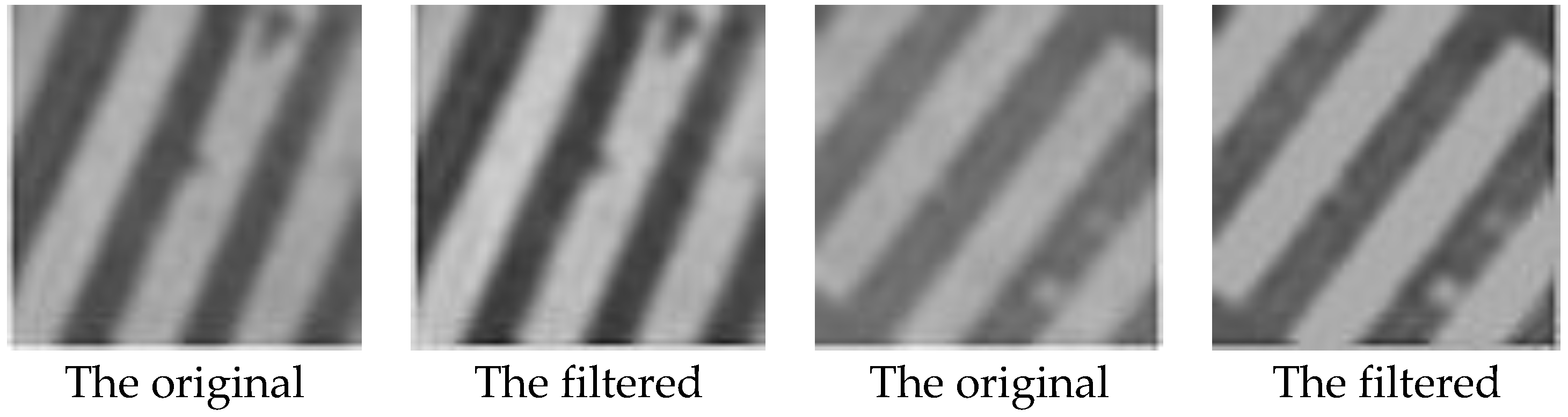
- Tan, D. Image enhancement based on adaptive median filter and Wallis filter. In Proceedings of the 4th National Conference on Electrical, Electronics and Computer Engineering, Xi’an, China, 12–13 December 2015; pp. 767–772.
- Gadkari, D. Image Quality Analysis Using GLCM. Master’s Thesis, University of Central Florida, Orlando, FL, USA, 2004. [Google Scholar]
- Lindeberg, T. Scale-space theory: A basic tool for analyzing structures at different scales. J. Appl. Stat. 1994, 21, 225–270. [Google Scholar] [CrossRef]
- Lindeberg, T. Feature detection with automatic scale selection. Int. J. Comput. Vis. 1998, 30, 79–116. [Google Scholar] [CrossRef]
- Lowe, D.G. Object recognition from local scale-invariant features. In Proceedings of the Seventh IEEE International Conference on Computer Vision, Kerkyra, Greece, 20–27 September 1999; pp. 1150–1157.
- Marr, D.; Hildreth, E. Theory of edge detection. Proc. R. Soc. Lond. B Biol. Sci. 1980, 207, 187–217. [Google Scholar] [CrossRef] [PubMed]
- Lowe, D.G. Distinctive image features from scale-invariant keypoints. Int. J. Comput. Vis. 2004, 60, 91–110. [Google Scholar] [CrossRef]
- Lee, T.S. Image representation using 2D Gabor wavelets. IEEE Trans. Pattern Anal. Mach. Intell. 1996, 18, 959–971. [Google Scholar]
- Turner, M.R. Texture discrimination by Gabor functions. Biol. Cybern. 1986, 55, 71–82. [Google Scholar] [PubMed]
- Guo, B.; Huang, X.; Zhang, F.; Sohn, G. Classification of airborne laser scanning data using Jointboost. ISPRS J. Photogramm. Remote Sens. 2015, 100, 71–83. [Google Scholar] [CrossRef]
- Stefan, A.; Athitsos, V.; Yuan, Q.; Sclaroff, S. Reducing Jointboost-based multiclass classification to proximity search. In Proceedings of the IEEE Conference on Computer Vision and Pattern Recognition, Miami, FL, USA, 20–25 June 2009; pp. 589–596.
- Fletcher, R.; Powell, M.J. A rapidly convergent descent method for minimization. Comput. J. 1963, 6, 163–168. [Google Scholar] [CrossRef]
- Manjunath, B.S.; Ohm, J.-R.; Vasudevan, V.V.; Yamada, A. Color and texture descriptors. IEEE Trans. Circuits Syst. Video Technol. 2001, 11, 703–715. [Google Scholar] [CrossRef]
- Bai, X.; Zhou, F. Analysis of new top-hat transformation and the application for infrared dim small target detection. Pattern Recognit. 2010, 43, 2145–2156. [Google Scholar] [CrossRef]
- Otsu, N. A threshold selection method from gray-level histograms. Automatica 1975, 11, 23–27. [Google Scholar]


| Dataset I (Blocks) | Dataset II (Blocks) | Dataset III (Blocks) | ||||||||||
|---|---|---|---|---|---|---|---|---|---|---|---|---|
| a | b | c | d | a | b | c | d | a | b | c | d | |
| correct | 426 | 384 | 375 | 120 | 247 | 62 | 331 | 586 | 284 | 392 | 323 | 327 |
| wrong | 14 | 2 | 4 | 3 | 4 | 3 | 55 | 4 | 0 | 9 | 4 | 2 |
| omission | 46 | 55 | 23 | 23 | 4 | 6 | 69 | 259 | 68 | 76 | 72 | 41 |
| Image A (478 Blocks) | Image B (382 Blocks) | |||||
|---|---|---|---|---|---|---|
| GLCM | 2D Gabor | Both | GLCM | 2D Gabor | Both | |
| correct | 316 | 337 | 372 | 294 | 334 | 345 |
| wrong | 6 | 1 | 0 | 0 | 4 | 0 |
| omission | 162 | 141 | 106 | 88 | 48 | 37 |
© 2016 by the authors; licensee MDPI, Basel, Switzerland. This article is an open access article distributed under the terms and conditions of the Creative Commons Attribution (CC-BY) license (http://creativecommons.org/licenses/by/4.0/).
Share and Cite
Sun, Y.; Zhang, F.; Gao, Y.; Huang, X. Extraction and Reconstruction of Zebra Crossings from High Resolution Aerial Images. ISPRS Int. J. Geo-Inf. 2016, 5, 127. https://doi.org/10.3390/ijgi5080127
Sun Y, Zhang F, Gao Y, Huang X. Extraction and Reconstruction of Zebra Crossings from High Resolution Aerial Images. ISPRS International Journal of Geo-Information. 2016; 5(8):127. https://doi.org/10.3390/ijgi5080127
Chicago/Turabian StyleSun, Yanbiao, Fan Zhang, Yunlong Gao, and Xianfeng Huang. 2016. "Extraction and Reconstruction of Zebra Crossings from High Resolution Aerial Images" ISPRS International Journal of Geo-Information 5, no. 8: 127. https://doi.org/10.3390/ijgi5080127
APA StyleSun, Y., Zhang, F., Gao, Y., & Huang, X. (2016). Extraction and Reconstruction of Zebra Crossings from High Resolution Aerial Images. ISPRS International Journal of Geo-Information, 5(8), 127. https://doi.org/10.3390/ijgi5080127