Abstract
Smart mobility has emerged as a sustainable solution to the challenges of traffic congestion and environmental pollution in cities. Within this concept, Urban Air Mobility (UAM) offers a promising approach to three-dimensional (3D) urban transportation. However, existing UAV path planning studies have primarily focused on obstacle avoidance in low-altitude airspace for small UAVs, with limited consideration of continuous and dynamic risks such as meteorological conditions. As UAM operates at higher altitudes than small UAVs, it is essential to expand the range of flight risks considered in path planning to ensure safe navigation. This study proposes a voxel-based optimal path planning method that integrates multiple flight risks to support various types of UAVs, including those in UAM systems. The proposed method generates a voxel-based flight risk map and extends a two-dimensional (2D) wavefront algorithm into a 3D voxel-based algorithm for deriving optimal paths. Validation through two scenarios, designed in a virtual 3D urban model, demonstrated a 57.59% reduction in the total flight risk index and a 40.72% increase in path length compared with the collision-free path. These results indicate that the proposed method effectively enhances the safety and reliability of UAV navigation in complex urban environments.
1. Introduction
Recently, as traffic congestion and environmental pollution problems have intensified in cities, the concept of smart mobility has emerged as a solution. Smart mobility is a solution that leverages advanced technologies to enhance the efficiency, accessibility, and sustainability of urban transportation systems []. Among these, three-dimensional (3D) urban transportation systems integrating aerial mobility are considered a potential alternative, with Urban Air Mobility (UAM) constituting a representative example. UAM is a transportation system that employs electric Vertical Takeoff and Landing (eVTOL) Unmanned Aerial Vehicles (UAVs) to carry passengers and cargo. Unmanned vehicles such as UAVs require both reactive navigation, which relies on real-time sensor measurements to react fast to concerning objects in the environment, and path planning, which enables path generation toward predetermined goals within a known environment []. This article focuses on the issue of path planning.
Small UAVs, which have been the subject of most existing studies, generally operate in low-altitude airspace below 400 feet [,]. Accordingly, UAV path planning research has primarily focused on avoiding obstacles such as buildings and structures []. However, as illustrated in Figure 1, UAVs in the UAM system operate at higher altitudes, where the influence of ground obstacles is reduced. At such altitudes, representing space simply as free or obstacle is no longer sufficient to describe the actual flight environment. Therefore, a more comprehensive path planning approach is required to consider various environmental factors, such as meteorological conditions.
Figure 1.
Airspace classification of UAVs, UAMs, and conventional aircraft.
Addressing multiple flight risks requires a data structure capable of integrally representing and computing diverse forms of risk. In this study, a voxel model is employed, which enables the precise representation of complex 3D spaces while also supporting flexible resolution adjustment and rapid updating of dynamic information []. In addition, since the topological relationships between voxels are implicitly defined, adjacent voxels can be efficiently identified through simple indexing during path planning. However, previous UAV path planning studies have generally converted voxel centers into nodes and represented node relations as edges to apply graph-based algorithms such as Dijkstra and A* [,]. These algorithms not only require explicit conversion of voxels into graph structures but also demand the management of adjacency relationships through separate search data structures, resulting in additional memory and computational costs []. Sampling-based algorithms can improve computational efficiency by reducing the search space. However, they are limited in achieving global optimality, particularly in tasks requiring stability and reliability []. As UAVs remain in the early stages of commercialization, ensuring robust and consistent flight performance is essential in path planning.
This study aims to derive an optimal path applicable to various types of UAVs, accounting for diverse forms of risk. To achieve this, a voxel-based optimal path planning method is proposed. The scope of this study is as follows. First, a flight risk map is generated by quantifying various risks affecting UAV flight, based on the voxel model. Second, the wavefront algorithm, a 2D cell-based method, is extended and adapted into a 3D voxel-based approach to define an optimal path from the flight risk map. Finally, the safety of the derived optimal path is quantitatively validated.
2. Related Works
Path planning mainly consists of two steps: environmental modeling and path searching []. Because environmental modeling directly influences the performance of path searching, defining and representing risks within urban airspace is an important aspect of research. Accordingly, this study reviews risk assessment for UAV Path planning and examines the path search algorithm.
2.1. Risk Assessment for UAV Path Planning
Previous studies on UAV path planning have primarily focused on obstacle avoidance in low-altitude airspace. Specifically, terrain [], buildings [,,], no-fly zones [,], and signal interference zones [] have been considered as risks. In addition, the analysis of meteorological risks is also required, as UAVs are smaller and lighter than conventional aircraft and therefore more sensitive to adverse meteorological factors []. Accordingly, some studies have attempted to incorporate weather risk into path planning []. However, such efforts remain relatively limited compared with obstacle-focused UAV path planning studies. Moreover, studies that simultaneously consider both obstacle and weather risks in path planning are scarce.
Various environment modeling techniques have been employed to incorporate risks into path planning. For instance, obstacles have been modeled by converting LiDAR data into meshes [] or transforming 3D urban building data into voxels []. These techniques are typically designed for individual risks and are therefore limited in modeling multiple risks simultaneously. Thus, some studies have employed a risk map to quantitatively evaluate diverse risks [,]. In a 2D environment, the risk map discretizes urban space into cells, enabling the integration of diverse risks into a composite index. This allows the spatial distribution of diverse risks to be represented quantitatively at the cell level. Building on this concept, this study develops a voxel-based risk map that integrates both obstacle and weather risks into path planning.
2.2. Path Search Algorithm
Traditionally, path searching algorithms are categorized into graph-based and cell-based approaches.
2.2.1. Graph-Based Approach
The graph-based approach searches for paths on a graph composed of nodes and edges and has therefore been widely applied to route-finding in irregular environments such as road networks []. However, as the dimensionality increases and path planning over larger areas becomes necessary, such graph-based algorithms face a fundamental trade-off between computational tractability and continuous-space optimality []. Higher spatial resolution enables more precise paths approximating the optimal solution, although the search data structure that stores adjacency relationships (e.g., adjacency lists or adjacency matrices) expands exponentially, leading to a rapid increase in memory consumption and computational cost []. Due to these limitations, graph-based algorithms have evolved toward enhancing efficiency by reducing the search space.
The Dijkstra algorithm [] is a classical method for solving the shortest-path problem, which iteratively updates the minimum distance from the start node to all other nodes until the end node is reached. Although this algorithm guarantees global optimality, it is limited by high computational complexity because it requires exploring all nodes.
The A* algorithm [] extends Dijkstra’s method by introducing a heuristic function to reduce the search space and improve computational efficiency. It prioritizes exploration toward the end node based on an evaluation function defined as f(n) = g(n) + h(n), where g(n) represents the actual cost from the start node to the current node, and h(n) denotes the estimated cost from the current node to the end node. While this approach offers greater efficiency than Dijkstra’s algorithm, it guarantees optimality only when the heuristic function satisfies both consistency and admissibility conditions.
Recently, the sampling-based approach has gained attention for path planning in high-dimensional spaces. Representative algorithms include the Probabilistic Roadmap (PRM) [], Expansive Space Trees (EST) [], and Rapidly Exploring Random Trees (RRT) []. These algorithms generate random samples within the planning space to construct an abstracted graph that simplifies the overall search domain. Such approaches may produce different solutions for the same problem due to the stochastic nature of the sampling process. This inherent randomness makes them unsuitable for scenarios that require stability and reliability [].
2.2.2. Cell-Based Approach
The cell-based approach performs path searching within a planning space discretized into uniformly sized cells. Therefore, it has been widely used for path planning in structured and large-scale environments such as airspace []. Cells have inherent consistency and regularity, allowing adjacency relationships to be represented simply and intuitively []. Consequently, cell-based algorithms do not require explicit definitions of the relationships between adjacent cells. In general, adjacency in 2D cells is represented by 4-neighborhood or 8-neighborhood structures, whereas in 3D voxels, it is extended to a 26-neighborhood, which can be easily identified through indexing []. Because the topological relationships between cells are clearly defined, the cell-based approach provides reliable spatial data support for path planning []. Nevertheless, because the movement is limited, the resulting paths often exhibit a zigzag pattern, causing the actual travel distance to be exaggerated []. Thus, many studies have adopted the cell-based approach by integrating complementary techniques to address this limitation.
Representative cell-based algorithms include the cellular automata (CA) and the wavefront algorithm []. CA assigns a state (e.g., empty space, obstacle, active, or inactive) to each cell and updates it iteratively based on predefined transition rules, gradually forming a feasible path []. Since its simple implementation and suitability for parallel computation, CA has been applied to various fields such as robot path planning [] and emergency evacuation modeling []. However, its performance is highly dependent on the design of the transition rules.
The wavefront algorithm propagates cumulative distances from the destination to the origin, and the shortest path is then obtained by tracing the wavefront gradient. Because this algorithm avoids local optima and guarantees a global optimal path, it has been widely adopted in collision-free path planning [,]. However, the traditional wavefront algorithm classifies cells simply as obstacles or free spaces and assigns equal distance weights to all adjacent cells during propagation, thereby limiting the accurate representation of actual travel distance []. In the field of GIS, this algorithm has been enhanced by assigning different distance weights according to adjacent directions and by penalizing obstacles instead of completely excluding them, thereby enabling path searching in complex environments []. Nevertheless, because this approach is designed for 2D cells, it cannot be directly employed for 3D path searching.
To address these limitations, this study extends the wavefront algorithm into 3D based on a voxel structure, ensuring global optimality while enabling efficient neighbor identification through simple indexing. In addition, it introduces a post-processing procedure to mitigate the distance exaggeration inherent in the voxel structure. The proposed method is suitable for UAV path planning in complex and large-scale urban airspaces and provides a novel solution to ensure the safety and reliability required in the early stage of UAV commercialization.
3. Proposed Method
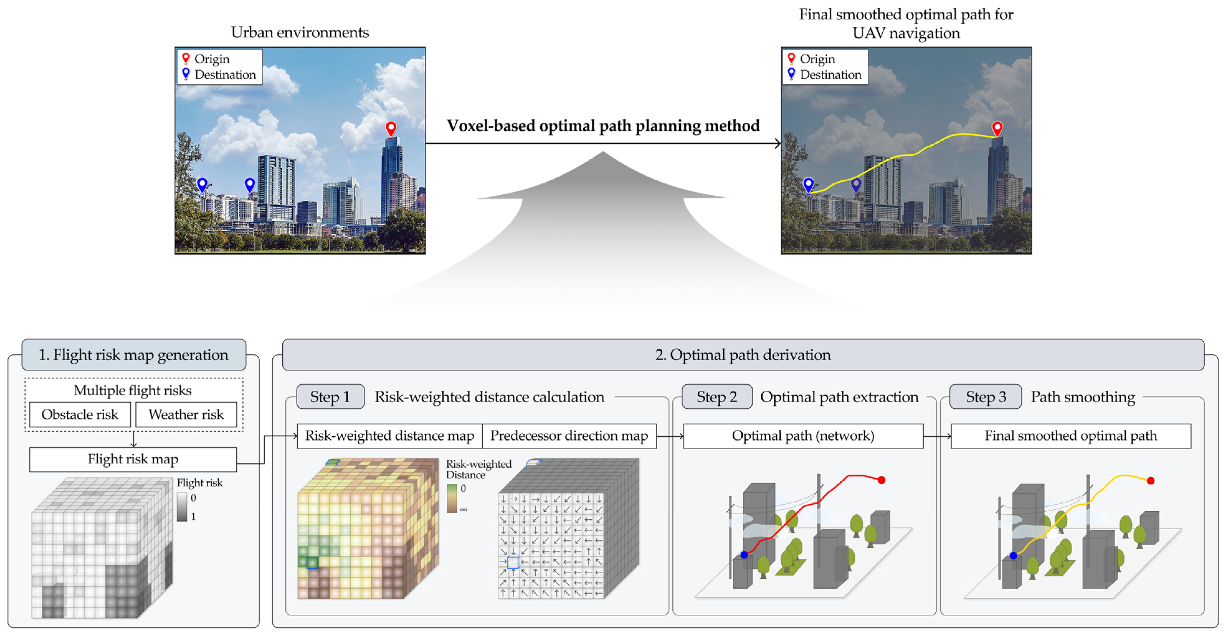
This study proposes a voxel-based optimal path planning method for deriving the optimal path applicable to various types of UAVs. As illustrated in Figure 2, the proposed method consists of two main phases. In the first phase, various forms of flight risk in urban environments are quantitatively assessed to generate a voxel-based flight risk map. In the second phase, this map is employed to derive an optimal path in three steps.
Figure 2.
Schematic diagram of the voxel-based optimal path planning method for UAV navigation.
3.1. Flight Risk Map Generation
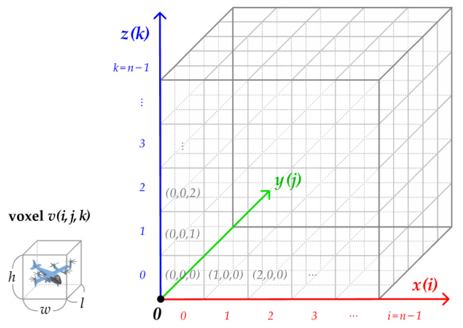
This study introduces the concept of the risk map [] to quantitatively evaluate diverse flight risks. The flight risk map is constructed based on a voxel model and illustrated in Figure 3. Each voxel is an equidistant cube representing a specific location in urban space, identified by local coordinates (i, j, k) within a right-handed Cartesian coordinate system. The voxel size is generally determined according to the actual size of the reference vehicle [].
Figure 3.
Conceptual representation of the voxel-based flight risk map.
Each voxel vi,j,k is assigned a flight risk index R(vi,j,k), which quantifies the level of risk associated with UAV flights within that space. The flight risk index is defined as a real number in the interval [0, 1]. R = 0 corresponds to a risk-free level suitable for safe UAV flight, whereas R = 1 denotes an extreme risk level where flight is practically infeasible. The flight risk index is calculated by integrating both obstacle risk, which has been widely considered in previous studies [,,,], and weather risk [,]. However, this study focuses on presenting a fundamental framework for integrating different types of risk into a voxel model, and the detailed process of converting real-world risk data into a voxel-based representation is beyond the scope of this study.
The obstacle risk Robstacle(vi,j,k) is defined as a binary indicator that takes the value 1 if any obstacle exists within voxel v, and 0 otherwise. The weather risk Rweather(vi,j,k) is defined as a continuous indicator representing the state of meteorological factors, such as cloud cover and precipitation. Each meteorological factor wm(vi,j,k) is required to be spatially interpolated to the same voxel size and normalized to the interval [0, 1] using min–max normalization before its inclusion in the flight risk map. The weather risk is expressed as a weighted sum of these meteorological factors, where the weights can alternatively be determined in proportion to the relative risk level that each meteorological factor poses to UAV flight through decision-making methods such as the Analytic Hierarchy Process (AHP) [].
where is the total number of considered meteorological factors, is the normalized risk value [0, 1] of meteorological factor at , and is the weight for meteorological factor .
Finally, the flight risk index R(vi,j,k) is defined as follows. First, obstacle risk is used to determine the feasibility of UAV flight within a voxel. If flight is considered infeasible (Robstacle(vi,j,k) = 1), then R(vi,j,k) takes the value 1. Conversely, if flight is feasible (Robstacle(vi,j,k) = 0), the weather risk is additionally incorporated to account for the potential influence of meteorological conditions on UAV flight, thereby computing the relative level of flight risk. This integration is expressed in Equation (2) and performed by voxel calculations (Figure 4).
Figure 4.
Voxel calculation for flight risk map generation.
3.2. Optimal Path Derivation
The optimal path is derived using Algorithm 1. The proposed algorithm takes the flight risk map R(v), the origin O, the destination D, and voxel size s as inputs. It generates the final smoothed optimal path G* from the origin to the destination in three steps.
| Algorithm 1 Optimal path derivation |
| Input: flight risk R(v), origin O, destination D, voxel size s Output: final smoothed optimal path G* 1: Calculate risk-weighted distance RD(v), predecessor direction PD(v) by Algorithm 2. 2: Extract optimal path G by Algorithm 3. 3: Calculate final smoothed optimal path G* by []. |
3.2.1. Risk-Weighted Distance Calculation
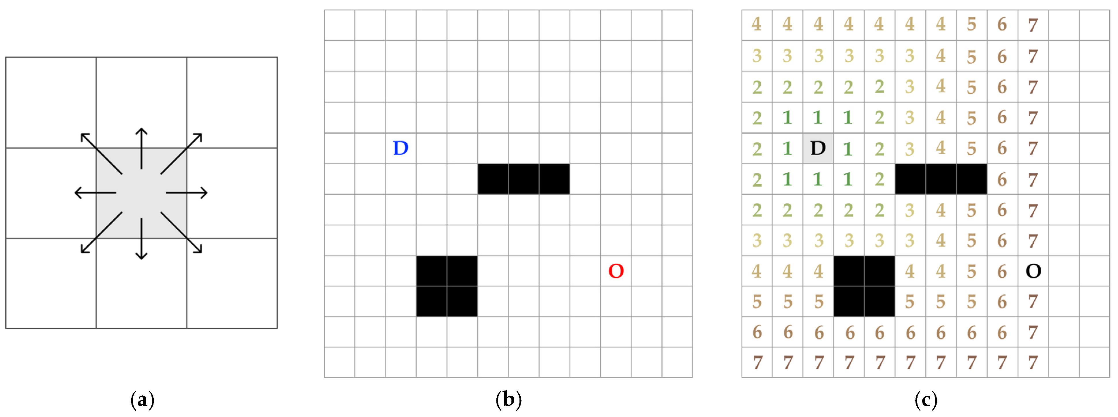
In the first step, the risk-weighted distance from the destination to each voxel is calculated, representing the cumulative travel distance that incorporates flight risks. To achieve this, the wavefront algorithm, a 2D cell-based method, is extended and adapted into a 3D voxel-based method. The wavefront algorithm propagates the cumulative distances from the destination toward the origin through free-space cells, excluding obstacles []. Each cell is connected to its 8-neighborhood, so the cumulative distance is propagated along these eight directions. These adjacency relationships can be efficiently identified through simple indexing without the need for an additional search data structure, achieving a time complexity of O(1) per operation, which is more efficient than graph-based algorithms. Once the propagation is completed, the shortest path can be identified within the cell-based environment (Figure 5). Because the wavefront algorithm is based on a simple principle, it operates robustly even in environments containing complex obstacles and guarantees the globally minimum cumulative distance path []. However, the traditional wavefront algorithm assigns equal weights to all directions during propagation, which limits its ability to accurately represent the actual travel distance [].
Figure 5.
Traditional wavefront algorithm: (a) 8-neighborhood of a cell, (b) example of grid environment with obstacles, and (c) propagation of the wavefront algorithm.
To overcome the limitations of the traditional wavefront algorithm, this study further develops the cell-based modified wavefront algorithm, implemented in ESRI’s ArcGIS Pro 3.4.0 as the cost distance tool [], by extending it into a 3D voxel-based algorithm that incorporates the different travel distances associated with adjacent directions. Each voxel has 26 adjacent voxels, consisting of 6 face-adjacent, 12 edge-adjacent, and 8 vertex-adjacent voxels (Figure 6). During propagation, distance weights corresponding to the Euclidean distances between voxels are assigned to each adjacent direction as follows.
Figure 6.
26 adjacencies of a voxel: (a) 6 face-adjacent, (b) 12 edge-adjacent, and (c) 8 vertex-adjacent.
Thus, the risk-weighted distance from voxel v to its adjacent voxel u is calculated as follows.
where is the risk-weighted distance of each voxel, is the flight risk index of each voxel, is the voxel size (m), and is the travel distance between two voxels, which can be calculated based on Equation (3).
The pseudocode for the risk-weighted distance calculation algorithm is presented in Algorithm 2. The algorithm receives the flight risk R(v) and destination D as input, where D can be a single voxel or multiple voxels. It produces risk-weighted distance RD(v), the minimum risk-weighted distance required to travel from D to each voxel v. For path extraction in the next step, predecessor direction PD(v) is also recorded, indicating the direction from which voxel v was reached.
The algorithm consists of two stages: initialization and propagation. At the initialization stage, RD(v) for all voxels is set to infinity, and the PD(v) is set to zero. In addition, three temporary variables, finalized, direction, and ActiveList are initialized.
- Finalized (v): A Boolean variable that indicates whether RD(v) of voxel v has been finalized. Once it is set to True, RD(v) remains fixed and is no longer updated.
- Direction (v): A variable that stores the current predecessor direction of each voxel v before the final assignment of PD(v).
- ActiveList: The set of candidate voxels whose RD(v) has not yet been finalized, storing their RD(v), coordinates (i, j, k), and direction.
After initialization, propagation continues iteratively from the destination D until all reachable voxels are finalized and the ActiveList is empty. Lines 7–11 set RD(d) and PD(d) to zero for each voxel d in D and insert d into the ActiveList as an initial active voxel. The iterative loop, described in Lines 13–31, extracts the voxel v with the minimum RD(v) from the ActiveList. If v has already been finalized, it is skipped. Otherwise, RD(v) is finalized, and PD(v) is updated. Subsequently, the 26-neighborhood of v is examined to propagate the wavefront into adjacent voxels. For each neighborhood u that is within bounds and has not yet been finalized, a tentative risk-weighted distance RD′(u) is calculated using Equation (4). If RD’(u) is smaller than the current RD(u), the corresponding entry in the ActiveList is updated by decreasing its value RD’(u). In addition, direction(u) is updated to reflect the current direction’(u). This iterative process propagates the wavefront while minimizing the cumulative distance and accounting for flight risk. At the end of propagation, RD(v) and PD(v) are finalized for all voxels.
| Algorithm 2 Risk-weighted distance calculation |
| Input: flight risk R(v), destination D, voxel size s Output: risk-weighted distance RD(v), predecessor direction PD(v) 1: Initialize RD(v) ← ∞ 2: Initialize PD(v) ← 0 3: Initialize finalized(v) ← False 4: Initialize direction(v) ← 0 5: Initialize ActiveList ← [] 6: 7: for each d ∈ D do 8: RD(d) ← 0 9: PD(d) ← 0 10: Insert d into ActiveList as (RD(d), d(i,j,k), PD(d)) 11: end for 12: 13: while ActiveList not empty do 14: Extract voxel v with minimum RD(v) from ActiveList as (RD(v), v, direction) 15: if finalized(v) then 16: continue 17: end if 18: finalized(v) ← True 19: PD(v) ← direction(v) 20: for each voxel u in the 26-neighborhood of v do 21: if u is out of bounds or finalized(u) then 22: continue 23: end if 24: Calculate RD’(u) by Equation (4) 25: if RD’(u) < RD(u) then 26: Decrease-Key of u in ActiveList to RD(u) 27: direction’(u) ← direction(u→ v) 28: Update u in ActiveList its direction(u) to direction’(u) 29: end if 30: end for 31: end while 32: 33: return RD(·), PD(·) |
To improve propagation efficiency, the ActiveList is implemented as a min-heap-based priority queue. In the traditional wavefront algorithm, which assigns equal distance weights to all free-space cells, propagation proceeds uniformly. Therefore, the ActiveList is typically implemented as a queue that processes cells in their order of visitation []. In this study, however, all voxels are associated with the flight risk R(v) and assigned different distance weights according to the adjacency direction, resulting in non-uniform propagation. The priority queue allows extracting the voxel v with the minimum RD(v) in O(log N) time per iteration, significantly enhancing the computational efficiency in large-scale voxel spaces compared to a simple list structure that requires O(n) time per operation.
3.2.2. Optimal Path Extraction
In the second step, the optimal path is extracted based on the predecessor direction. The pseudocode for the optimal path extraction algorithm is presented in Algorithm 3. The algorithm takes the origin O, destination D, and predecessor direction PD(v) as input and generates the optimal path G. Lines 7–11 reconstruct the voxel-level path by sequentially tracing PD(v) from the origin to the destination. Subsequently, Lines 13–15 convert the voxel-based optimal path into a network structure by representing the center of each voxel as a node and defining adjacencies between voxels as edges.
| Algorithm 3 Optimal path extraction |
| Input: origin O, destination D, predecessor direction PD(v) Output: optimal path G 1: Initialize path ← [] 2: Initialize node ← {}, edge ← {} 3: 4: current ← O 5: Insert current into path 6: 7: while PD(current) ≠ 0 do 8: Convert OD(current) into (Δx, Δy, Δz) 9: current ← current + (Δx, Δy, Δz) 10: Insert current into path 11: end while 12: 13: node ← {center(p) | p ∈ path} 14: edge ← {(pathi−1, pathi) | i = 1,…, |path| − 1} 15: G ← (node, edge) 16: 17: return G |
3.2.3. Path Smoothing
In the third step, path smoothing is applied to the previously generated optimal path. Because of the limited movement directions of the voxel model (26-neighborhood), the optimal path often appears in a zigzag pattern, which is unsuitable for practical UAV navigation. Such a path not only exaggerates the travel distance [] but also fails to reflect the dynamic constraints of UAVs, thereby limiting its operational feasibility.
To address these issues, cubic B-splines have been widely adopted in engineering and academic studies because they ensure continuity of position, velocity, and acceleration while maintaining a favorable balance between computational efficiency and curve smoothness []. In addition, their narrow local support allows adjustments to control points to influence only nearby segments of the curve [], which is advantageous for local obstacle avoidance. Therefore, this study adopts the cubic B-spline smoothing method based on local waypoint interpolation proposed by []. This method smooths curves while enabling local control to prevent intersections with obstacles (R(v) = 1).
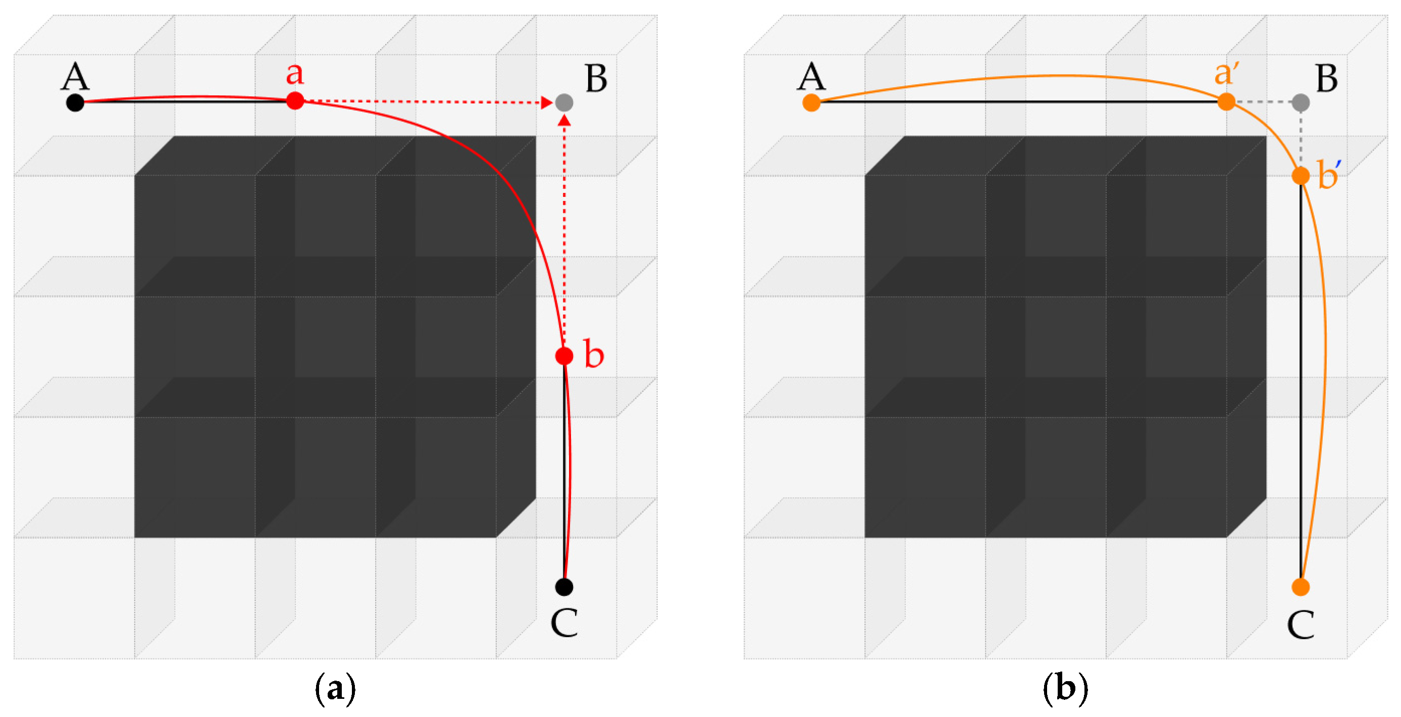
The smoothing process is illustrated in Figure 7. In this figure, black voxels represent obstacles (R(v) = 1), while control points A, B, and C correspond to nodes of the optimal path G. Initially, cubic B-spline smoothing is applied to three control points, and potential intersections with obstacles are examined. If the curve intersects the obstacle, intermediate control points (a, b) are inserted, and the smoothing is reapplied (Figure 7a). If the regenerated curve (A–a–c–C) still intersects an obstacle, the control points a and c are iteratively adjusted toward the direction of B until the intersection is eliminated. Once the obstacle is avoided, the control points are finalized, and the final smoothed path G* is derived (Figure 7b).
Figure 7.
Cubic B-spline smoothing based on local waypoint interpolation proposed by []: (a) inserting intermediate control points a and b when the curve intersects an obstacle, (b) final smoothed path after obstacle avoidance.
4. Implementation
4.1. Stepwise Implementation and Visualization of the Proposed Method
The proposed method was implemented in Python (version 3.10) to derive the optimal path applicable to various types of UAVs by considering diverse forms of flight risk in urban environments. Since this study focuses on developing a fundamental method for path planning that integrates multiple risks, voxelization of real-world spatial data is beyond its scope. Accordingly, the experimental validation was performed using synthetically generated sample data in the widely adopted NetCDF format [,], representing risks at the voxel-based layer.
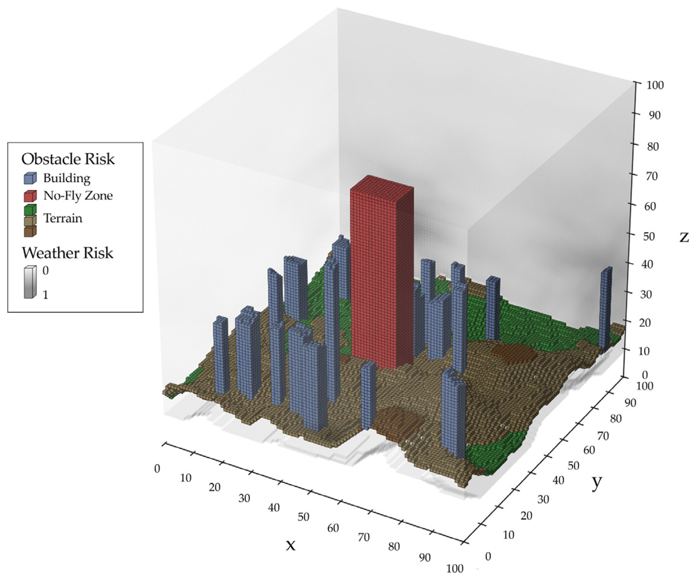
For the implementation, a 3D urban model was constructed, consisting of 100 × 100 × 100 voxels with a voxel size of 20 m (Figure 8). The voxel size was determined by the physical size of the representative UAM vehicle, the Joby S4. In this model, blue voxels represent buildings, red voxels represent no-fly zones, and green to brown voxels represent terrain with gradually increasing elevation. Each voxel was also assigned a weather risk within the range [0, 1], reflecting meteorological conditions such as cloud cover and precipitation, for which equal weights were applied across all meteorological factors due to the use of simulated data.
Figure 8.
Implementation environment of the voxel-based 3D urban model.
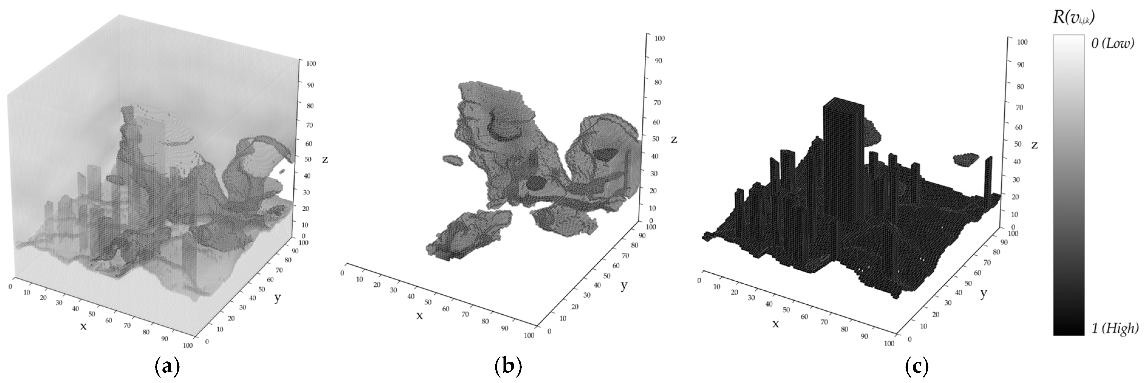
In the first phase, the flight risk R(v) was calculated by integrating both obstacle risk and weather risk. Figure 9 illustrates the spatial distribution of flight risk within the range [0, 1], categorized into three equal intervals. Voxels with obstacle risk were considered infeasible for flight (R(v) = 1), while the weather risk was incorporated in feasible voxels to determine their relative flight risk levels. Notably, the medium-level flight risk index was observed in areas located behind the no-fly zones.
Figure 9.
Flight risk index: (a) low level (0–0.333), (b) medium level (0.334–0.666), (c) high level (0.667–1.0).
In the second phase, the final smoothed optimal path G* from the origin to the destination was derived using the flight risk map in three steps. The origin and destinations were defined based on vertiport locations situated on building rooftops within the UAM system. Specifically, the origin was set at vertiport A (23, 74, 54), and the destinations were set at vertiport B (99, 87, 44) and vertiport C (89, 13, 46).
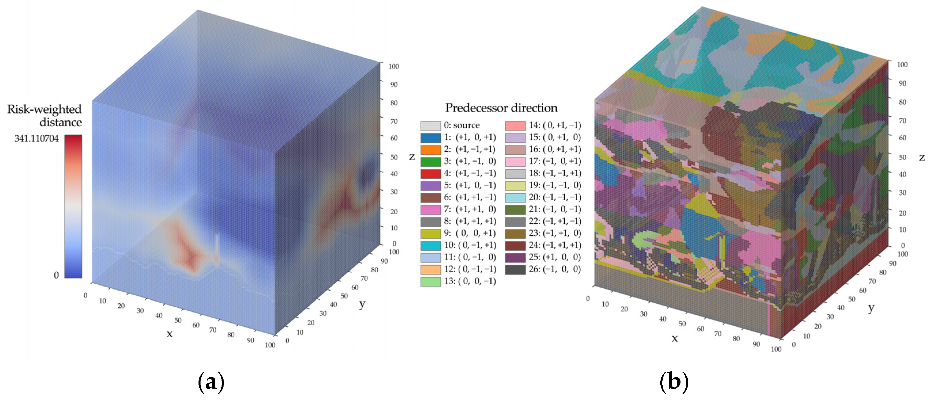
In the first step, the risk-weighted distance from the destination to each voxel was calculated. Figure 10 presents the spatial distribution of risk-weighted distance and predecessor direction. The risk-weighted distance represents the minimum cumulative distance that incorporates flight risk and is required to travel from vertiport B and C to each voxel, whereas the predecessor direction represents the direction from which voxel v was reached.
Figure 10.
(a) Risk-weighted distance map. (b) Predecessor direction map.
In the second step, the optimal path network from the origin to the destination was extracted based on the predecessor direction, as shown in Figure 11. Although the Euclidean distance between vertiport A and vertiport B was shorter, the optimal path was generated toward vertiport C to minimize overall flight risk.
Figure 11.
Optimal path extracted based on the predecessor direction map: (a) 3D view, (b) top view.
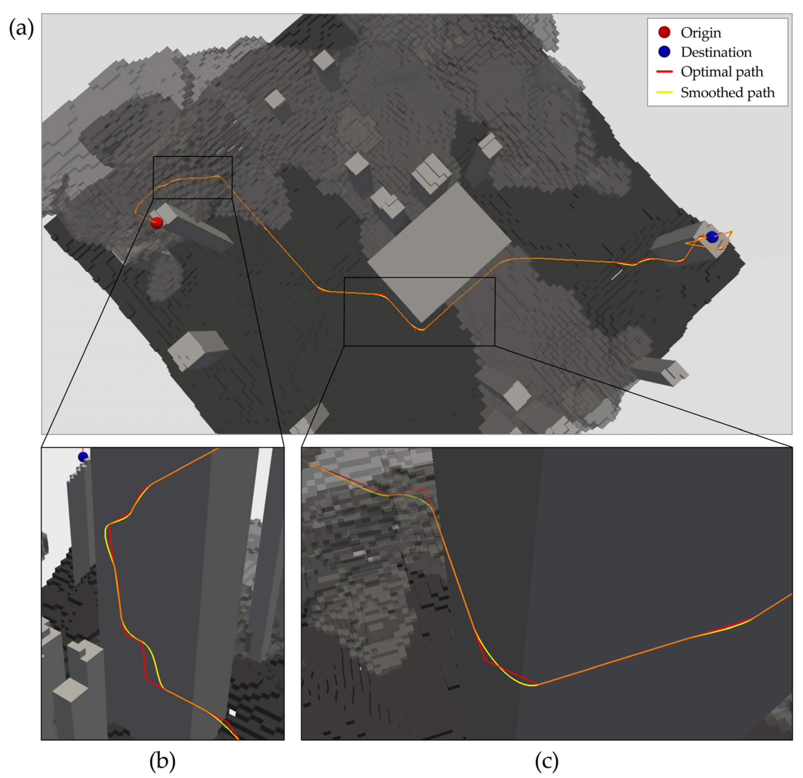
In the third step, cubic B-spline smoothing based on local waypoint interpolation [] was applied to the optimal path. The resulting final smoothed optimal path is shown in Figure 12. Due to the directional constraints imposed by the voxel model, the optimal path exhibited a zigzag pattern that is unsuitable for UAV flight. However, the final smoothed path was refined into a continuous and smooth trajectory while effectively avoiding collisions with obstacles.
Figure 12.
Final smoothed optimal path: (a) entire path, (b) enlarged view near the origin, and (c) enlarged view near the obstacle.
4.2. Quantitative Evaluation of Path Performance Under Experimental Scenarios
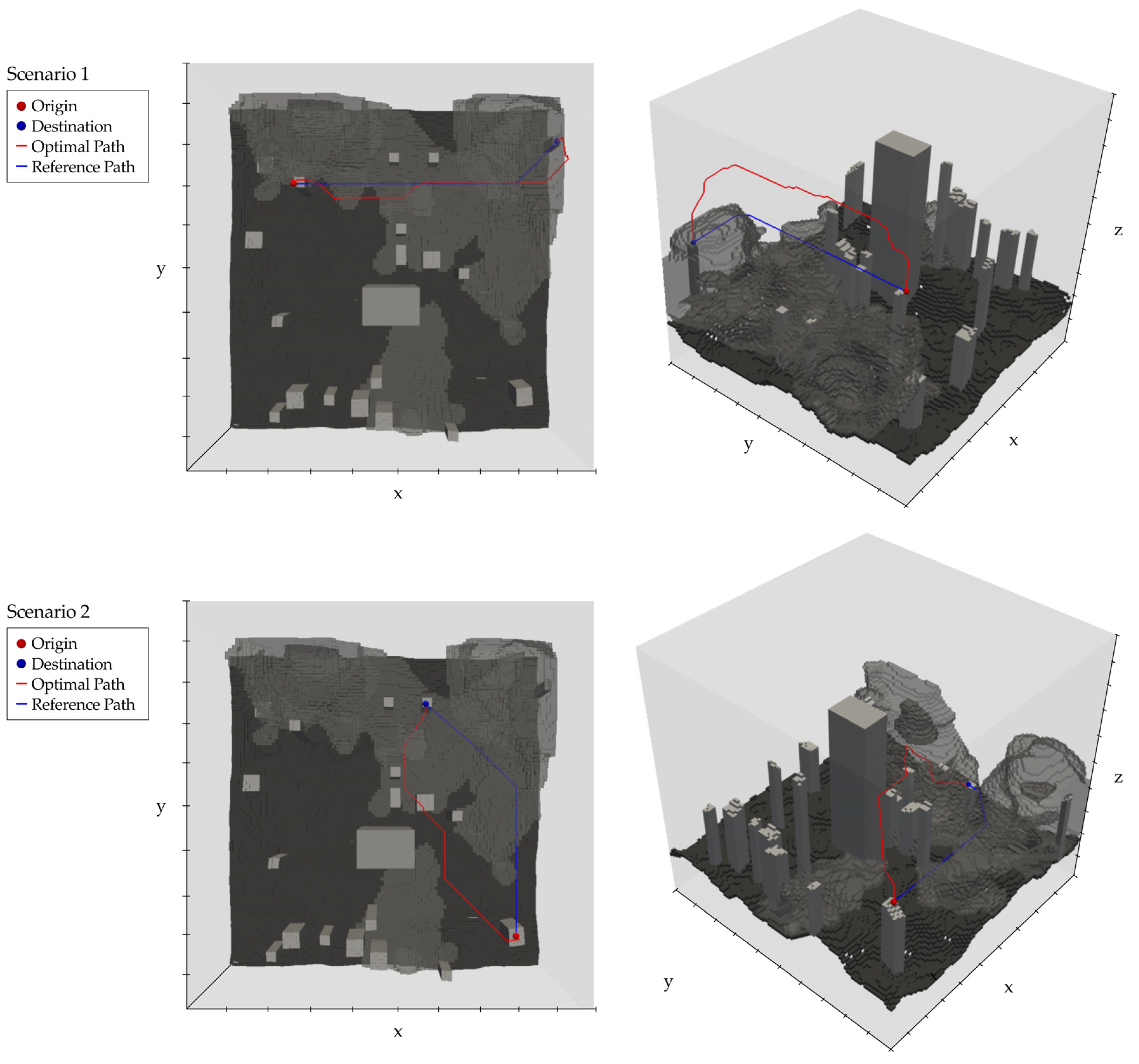
The two experimental scenarios were designed to analyze the differences in path length and safety between the optimal path derived from the proposed method and a reference path. The reference path was generated based on the principle of the traditional 2D wavefront algorithm, which classifies space only into obstacles and free cells, thereby producing a collision-free path without considering continuous risks. Each scenario was configured with different origin and destination points within the constructed 3D urban environment to examine the consistency of the results under different spatial configurations. In addition, the final smoothed path was compared to examine the effects of the post-processing procedure. The optimal path and reference path from the two scenarios are presented in Figure 13.
Figure 13.
Comparison of the optimal path and reference path generated by the proposed algorithm under two scenarios.
To quantitatively evaluate the safety of each path, a total flight risk index was calculated using the probabilistic risk assessment method proposed by []. Theoretically, this index is obtained by integrating the risk density function along the path. Since this study employs a voxel-based flight risk map, as in previous research, the index was computed by accumulating the voxel-based flight risk values using the following approximation equation. This index represents the total accumulated flight risk along the path and is a dimensionless quantity. It is derived from the summation of voxel-level risk density values normalized to the range [0, 1], rather than from a probability or a variable with physical units. Therefore, this index serves as a relative metric for comparing the safety of different paths under the same flight risk map.
where is the flight risk index in voxel , is the path length within voxel , and is the total number of voxels intersected by the path.
Specifically, the quantitative comparison of each path under two scenarios is summarized in Table 1. For the flight risk index, the total value, as computed by Equation (5), represents the total accumulated flight risk along the entire path, whereas the average value indicates the risk per meter, obtained by dividing the total risk by the path length. The minimum and maximum values correspond to the lowest and highest voxel-level flight risk values encountered along the path, respectively.
Table 1.
Quantitative comparison of the collision-free path, optimal path, and final smoothed optimal path under two scenarios of path length and risk metrics.
In Scenario 1, the optimal path was 44.813% (757.907 m) longer than the reference path, whereas the total flight risk index decreased by 56.586% (227.927). The average flight risk index, representing the risk per meter, also decreased by 70.168% (0.167), and both the minimum and maximum values were lower than those of the reference path. Furthermore, compared with the optimal path, the final smoothed optimal path showed a 1.477% (36.181 m) reduction in path length and a 0.293% (0.512) decrease in the total flight risk index. The average flight risk index slightly increased by 1.408% (0.001), and both the minimum and maximum values were unchanged.
A similar trend was observed in Scenario 2. The optimal path was 36.617% (624.099 m) longer than the reference path, whereas the total flight risk index decreased by 58.587% (188.128). The average flight risk index decreased by 69.681% (0.131), and both the minimum and maximum values were again lower than those of the reference path. Compared with the optimal path, the final smoothed optimal path exhibited a 2.242% (52.2 m) reduction in path length and a 2.756% (3.665) reduction in the total flight risk index. The average and minimum flight risk indices remained unchanged, while the maximum flight risk index slightly increased.
Overall, although the optimal path was longer than the reference path, it exhibited substantially lower total risk. In both scenarios, the rate of reduction in total flight risk index (57.59%) exceeded the rate of increase in path length (40.72%). This demonstrates that the proposed method effectively reduces flight risk despite a moderate increase in path length. Additionally, the smoothing method effectively mitigated the exaggerated distance inherent to voxel-based paths without causing any significant increase in flight risk.
5. Discussion
This section discusses the implications of the experimental results and highlights the methodological contributions of the proposed path planning approach.
The results demonstrate a quantifiable trade-off between path length and safety. Although the optimal path derived from the proposed method was moderately longer than the reference path, the substantial reduction in the total flight risk index highlights that the proposed algorithm effectively prioritizes flight safety over minimal path distance. While previous UAV path planning studies have primarily emphasized time-efficient [,,] or energy-efficient paths [,], the proposed method guarantees a globally optimal path in terms of safety. Therefore, it provides a new alternative for operations where safety and reliability are critical, such as early-stage UAM applications that are not yet fully commercialized. Furthermore, this approach may also be effective in various safety-critical scenarios, including autonomous delivery drones operating in densely populated areas or surveillance UAVs required to maintain stable flight under adverse weather conditions.
Compared with conventional UAV path planning approaches, the proposed method incorporates a broader set of flight risks into the path planning process. Previous studies have primarily considered limited categories of risks, such as terrain [], buildings and urban structures [,,], and no-fly zones [,]. While these studies provide essential foundations for safe navigation, they do not fully capture the diverse flight risks present in urban airspace. In contrast, the proposed approach explicitly integrates multiple flight risks, including meteorological conditions, by normalizing risk indicators and embedding them within the voxel structure. This integration provides a more realistic representation of urban airspace and offers flexibility to incorporate additional environmental or operational risks as relevant data become available. As a result, the method improves the robustness and situational awareness of UAV path planning across complex and variable flight conditions.
Furthermore, by extending the traditional 2D wavefront algorithm to a fully 3D voxel-based implementation, the proposed method reduces the need for explicit graph construction and adjacency management typically required in graph-based algorithms. The direct use of voxel adjacency relationships not only simplifies the computation process but also enhances scalability for large-scale urban airspace modeling. In addition, incorporating travel distances associated with adjacent directions enables a more realistic estimation of actual movement compared with conventional cell-based algorithms. Collectively, these enhancements suggest that the proposed method provides a theoretically grounded and computationally efficient foundation for safe path planning in complex 3D environments.
6. Conclusions
This study proposed a voxel-based optimal path planning method to support various types of UAVs, including those in UAM systems. The method integrates diverse forms of flight risk to ensure a globally optimal path in terms of safety, thereby providing a foundation for reliable navigation in complex 3D urban environments. Quantitative evaluation showed that the optimal path was approximately 40.72% longer than the reference path, while the total flight risk index decreased by 57.59%, demonstrating a substantial improvement in safety.
In the future, this study can be extended to the following aspects. First, future extensions may examine how the method can be balanced with other operational objectives, such as travel time and energy efficiency. Second, incorporating actual meteorological and environmental datasets could further clarify the robustness, reproducibility, and practical feasibility of the proposed method under realistic operational conditions. Third, additional analysis may be conducted to explore the computational implications of voxel resolution, particularly its influence on memory usage and processing efficiency. Such exploration may help identify an appropriate balance between spatial precision and computational cost, supporting the scalability and practical applicability of the proposed method in large-scale urban environments.
Author Contributions
Conceptualization, Jiyeong Lee and Min Jang; methodology, Jiyeong Lee, Min Jang and Dohee Kim; software, Min Jang; validation, Jiyeong Lee and Min Jang; formal analysis, Jiyeong Lee and Min Jang; investigation, Min Jang; resources, Jiyeong Lee and Min Jang; data curation, Min Jang; writing—original draft preparation, Min Jang; writing—review and editing, Jiyeong Lee and Min Jang; visualization, Jiyeong Lee, Min Jang and Dohee Kim; supervision, Jiyeong Lee; project administration, Jiyeong Lee; funding acquisition, Jiyeong Lee. All authors have read and agreed to the published version of the manuscript.
Funding
This work was supported by an Korea Agency for Infrastructure Technology Advancement (KAIA) grant funded by the Ministry of Land, Infrastructure and Transport (RS-2025-02317649, Implementation and Application of 3D Grid System for Advanced National Spatial Information).
Data Availability Statement
No new data were created or analyzed in this study. Data sharing is not applicable to this article.
Conflicts of Interest
The authors declare no conflicts of interest.
Abbreviations
The following abbreviations are used in this manuscript:
| UAM | Urban Air Mobility |
| eVTOL | Electric Vertical Takeoff and Landing |
| UAV | Unmanned Aerial Vehicle |
| 2D | Two-dimensional |
| 3D | Three-dimensional |
References
- Mitieka, D.; Luke, R.; Twinomurinzi, H.; Mageto, J. Smart Mobility in Urban Areas: A Bibliometric Review and Research Agenda. Sustainability 2023, 15, 6754. [Google Scholar] [CrossRef]
- Cabreira, T.M.; Brisolara, L.B.; Ferreira, P.R., Jr. Survey on Coverage Path Planning with Unmanned Aerial Vehicles. Drones 2019, 3, 4. [Google Scholar] [CrossRef]
- Federal Aviation Administration (FAA). Small Unmanned Aircraft Systems: 14 CFR Part 107—Operating Limitations for Small Unmanned Aircraft (§107.51). 2016. Available online: https://www.ecfr.gov/current/title-14/chapter-I/subchapter-F/part-107 (accessed on 22 September 2025).
- European Union Aviation Safety Agency (EASA). Easy Access Rules for Unmanned Aircraft Systems. 2024. Available online: https://www.easa.europa.eu/en/document-library/easy-access-rules/online-publications/easy-access-rules-unmanned-aircraft-systems (accessed on 22 September 2025).
- Zhang, H.; Tian, T.; Feng, O.; Wu, S.; Zhong, G. Research on Public Air Route Network Planning of Urban Low-Altitude Logistics Unmanned Aerial Vehicles. Sustainability 2023, 15, 12021. [Google Scholar] [CrossRef]
- Niu, L.; Wang, Z.; Lin, Z.; Zhang, Y.; Yan, Y.; He, Z. Voxel-Based Navigation: A Systematic Review of Techniques, Applications, and Challenges. ISPRS Int. J. Geo-Inf. 2024, 13, 461. [Google Scholar] [CrossRef]
- Chiciudean, V.; Oniga, F. Pathfinding in a 3D Grid for UAV Navigation. In Proceedings of the 2022 IEEE 18th International Conference on Intelligent Computer Communication and Processing (ICCP), Cluj-Napoca, Romania, 22–24 September 2022; IEEE: Piscataway, NJ, USA, 2022; pp. 305–311. [Google Scholar] [CrossRef]
- Valiente, G. Adjacency Maps and Efficient Graph Algorithms. Algorithms 2022, 15, 67. [Google Scholar] [CrossRef]
- Tang, Q.; Dou, W. An Effective Method for Computing the Least-Cost Path Using a Multi-Resolution Raster Cost Surface Model. ISPRS Int. J. Geo-Inf. 2023, 12, 287. [Google Scholar] [CrossRef]
- Zhang, H.-Y.; Lin, W.-M.; Chen, A.-X. Path Planning for the Mobile Robot: A Review. Symmetry 2018, 10, 450. [Google Scholar] [CrossRef]
- Tang, H.; Zhang, Y.; Mohmoodian, V.; Charkhgard, H. Automated flight planning of high-density urban air mobility. Transp. Res. Part C Emerg. Technol. 2021, 131, 103324. [Google Scholar] [CrossRef]
- Zhang, N.; Zhang, M.; Low, K.H. 3D path planning and real-time collision resolution of multirotor drone operations in complex urban low-altitude airspace. Transp. Res. Part C Emerg. Technol. 2021, 129, 103123. [Google Scholar] [CrossRef]
- Roseman, C.A.; Argrow, B.M. Weather hazard risk quantification for sUAS safety risk management. J. Atmos. Ocean. Technol. 2020, 37, 1251. [Google Scholar] [CrossRef]
- Teng, Y.; Wang, X.; Wang, L.; Yao, M. The Safety Risk Assessment Method for Logistics UAV Considering Environmental Impacts. In Proceedings of the 2024 IEEE International Conference on Unmanned Systems (ICUS), Nanjing, China, 18–20 October 2024; IEEE: Piscataway, NJ, USA, 2024; pp. 219–224. [Google Scholar] [CrossRef]
- Primatesta, S.; Rizzo, A.; la Cour-Harbo, A. Ground Risk Map for Unmanned Aircraft in Urban Environments. J. Intell. Robot. Syst. 2020, 97, 489–509. [Google Scholar] [CrossRef]
- Hu, X.; Pang, B.; Dai, F.; Low, K.H. Risk assessment model for UAV cost-effective path planning in urban environments. IEEE Access 2020, 8, 150162–150173. [Google Scholar] [CrossRef]
- Sohrabi, S.; Weng, Y.; Das, S.; German Paal, S. Safe Route-Finding: A Review of Literature and Future Directions. Accid. Anal. Prev. 2022, 177, 106816. [Google Scholar] [CrossRef] [PubMed]
- Andaryan, A.Z.; Bell, M.G.; Ramezani, M.; Geers, G. V*: An Efficient Motion Planning Algorithm for Autonomous Vehicles. arXiv 2025, arXiv:2508.06404. [Google Scholar] [CrossRef]
- Dijkstra, E. A note on two problems in connexion with graphs. Numer. Math. 1959, 4, 269–271. [Google Scholar] [CrossRef]
- Hart, P.E.; Nilsson, N.J.; Raphael, B. A formal basis for the heuristic determination of minimum cost paths in graphs. IEEE Trans. Syst. Sci. Cybern. 1968, 4, 100–107. [Google Scholar] [CrossRef]
- Kavraki, L.E.; Svestka, P.; Latombe, J.C.; Overmars, M.H. Probabilistic roadmaps for path planning in high-dimensional configuration spaces. IEEE Trans. Robot. Autom. 1996, 12, 566–580. [Google Scholar] [CrossRef]
- Hsu, D.; Kindel, R.; Latombe, J.C.; Rock, S. Randomized kinodynamic motion planning with moving obstacles. Int. J. Robot. Res. 2002, 21, 233–255. [Google Scholar] [CrossRef]
- LaValle, S.M. Rapidly-Exploring Random Trees: A New Tool for Path Planning. 1998. Available online: http://lavalle.pl/papers/Lav98c.pdf (accessed on 11 November 2025).
- Liu, L.; Wang, X.; Yang, X.; Liu, H.; Li, J.; Wang, P. Path Planning Techniques for Mobile Robots: Review and Prospect. Expert Syst. Appl. 2023, 227, 120254. [Google Scholar] [CrossRef]
- Sun, Y.; Li, H.; Tong, X.; Lei, Y.; Wang, D.; Guo, C.; Tang, J.; Shang, Y. A Multi-Unmanned Aerial Vehicle Fast Path-Planning Method Based on Non-Rigid Hierarchical Discrete Grid Voxel Environment Modeling. Int. J. Appl. Earth Obs. Geoinf. 2023, 116, 103139. [Google Scholar] [CrossRef]
- Goodchild, M.F. An evaluation of lattice solutions to the problem of corridor location. Environ. Plan. A 1977, 9, 727–738. [Google Scholar] [CrossRef]
- Murphy, R. Introduction to AI Robotics; MIT Press: Cambridge, MA, USA, 2019. [Google Scholar]
- Zelenka, J.; Kasanicky, T. Outdoor UAV Control and Coordination System Supported by Biological Inspired Method. In Proceedings of the 2014 23rd International Conference on Robotics in Alpe-Adria-Danube Region (RAAD), Smolenice, Slovakia, 3–5 September 2014; pp. 1–7. [Google Scholar] [CrossRef]
- Marchese, F.M. A directional diffusion algorithm on cellular automata for robot path-planning. Future Gener. Comput. Syst. 2020, 18, 983–994. [Google Scholar] [CrossRef]
- Ronchi, E. Developing and Validating Evacuation Models for Fire Safety Engineering. Fire Saf. J. 2021, 120, 103020. [Google Scholar] [CrossRef]
- Tang, C.; Liang, Y.; Yu, S.; Sun, R.; Zheng, J. Autonomous 3D Exploration of Indoor Environment Based on Wavefront Algorithm. In Proceedings of the 2020 IEEE International Conference on Networking, Sensing and Control (ICNSC), Nanjing, China, 30 October–2 November 2020; IEEE: Piscataway, NJ, USA, 2020; pp. 1–6. [Google Scholar] [CrossRef]
- Psotka, M.; Duchoň, F.; Roman, M.; Michal, T.; Michal, D. Global Path Planning Method Based on a Modification of the Wavefront Algorithm for Ground Mobile Robots. Robotics 2023, 12, 25. [Google Scholar] [CrossRef]
- Ghai, B.; Shukla, A. Wave Front Method Based Path Planning Algorithm for Mobile Robots. In Proceedings of the First International Conference on Information and Communication Technology for Intelligent Systems, Ahmedabad, India, 28–29 November 2015; Satapathy, S., Das, S., Eds.; Smart Innovation, Systems and Technologies; Springer: Cham, Switzerland, 2016; Volume 51, pp. 281–288. [Google Scholar] [CrossRef]
- ESRI. How Cost Distance Tools Work. Available online: https://desktop.arcgis.com/en/arcmap/10.4/tools/spatial-analyst-toolbox/how-the-cost-distance-tools-work.htm (accessed on 22 August 2025).
- Li, X.; Gao, X.; Zhang, W.; Hao, L. Smooth and collision-free trajectory generation in cluttered environments using cubic B-spline form. Mech. Mach. Theory 2022, 169, 104606. [Google Scholar] [CrossRef]
- Piegl, L.; Tiller, W. The NURBS Book, 2nd ed.; Springer: New York, NY, USA, 1996. [Google Scholar]
- Lv, T.; Fu, J.; Li, B. Design and Application of Multi-Dimensional Visualization System for Large-Scale Ocean Data. ISPRS Int. J. Geo-Inf. 2022, 11, 491. [Google Scholar] [CrossRef]
- Kaya, U.C.; Dogan, A.; Huber, M. A Probabilistic Risk Assessment Framework for the Path Planning of Safe Task-Aware UAS Operations. In Proceedings of the AIAA Scitech 2019 Forum, San Diego, CA, USA, 7–11 January 2019. [Google Scholar] [CrossRef]
- Paielli, R.A. Trajectory generation based on power for urban air mobility. Front. Aerosp. Eng. 2023, 2, 1278726. [Google Scholar] [CrossRef]
Disclaimer/Publisher’s Note: The statements, opinions and data contained in all publications are solely those of the individual author(s) and contributor(s) and not of MDPI and/or the editor(s). MDPI and/or the editor(s) disclaim responsibility for any injury to people or property resulting from any ideas, methods, instructions or products referred to in the content. |
© 2025 by the authors. Published by MDPI on behalf of the International Society for Photogrammetry and Remote Sensing. Licensee MDPI, Basel, Switzerland. This article is an open access article distributed under the terms and conditions of the Creative Commons Attribution (CC BY) license (https://creativecommons.org/licenses/by/4.0/).