Multi-Scale Non-Local Spatio-Temporal Information Fusion Networks for Multi-Step Traffic Flow Forecasting

Abstract

Traffic flow prediction is a crucial research area in traffic management. Accurately predicting traffic flow in each area of the city over the long term can enable city managers to make informed decisions regarding the allocation of urban transportation resources in the future. The existing traffic flow prediction models either give insufficient attention to the interactions of long-lasting spatio-temporal regions or extract spatio-temporal features in a single scale, which ignores the identification of traffic flow patterns at various scales. In this paper, we present a multi-scale spatio-temporal information fusion model using non-local networks, which fuses traffic flow pattern features at multiple scales in space and time, complemented by non-local networks to construct the global direct dependence relationship between local areas and the entire region of the city in space and time in the past. The proposed model is evaluated through experiments and is shown to outperform existing benchmark models in terms of prediction performance.

1. Introduction

Accurately predicting traffic flow has become crucial in the development and construction of smart cities [1]. The precise processing of urban traffic information and forecasting changes can enable city officials to understand current urban operations and make more efficient and effective management decisions [2,3,4]. In addition, the results of traffic flow prediction can be used to optimize the city’s land use [5], reduce traffic congestion [6], and optimize the location of functional areas [7], helping to develop a complete and comprehensive smart city system. The field of traffic flow prediction has progressed from traditional dynamical models [8] and statistical models [9,10,11] to models based on deep learning. Although better than traditional prediction models, the performance of these existing deep learning models still has some limitations.

Firstly, there are still limitations in traffic flow pattern recognition. Different urban areas serve different functions, and traffic patterns within these areas change over time. As shown in Figure 1, the areas marked in green illustrate traffic connectivity at a small scale, where a single area contains multiple road intersections with different road flow efficiencies and where a single area is connected to neighboring areas with road connections in a very short period of time to form its own traffic flow pattern. At a larger scale, the area is not only composed of roads, but may also contain different types of buildings. The zones marked in red represent the different functional areas of the city as a result of actual use, which may be work, residential, or commercial areas, and the traffic flows between these zones are influenced by the time of day and the road connections in the area. For example, on weekdays, the main traffic flows are between residential and commercial areas, and on weekends, the focus of traffic flows shifts to residential and consumer areas. If the road connections between areas are dense, the rate of change of traffic flow between the two will also be faster, while for larger spans between areas that need to build traffic connections through multiple intermediate areas, the change of traffic flow will be relatively slow. Capturing their specific traffic flow patterns at different scales will help the model to make accurate predictions of future traffic flow trends.

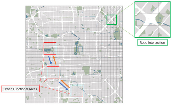
Figure 1. Differences in flows between regions at different scales.

The second limitation is the lack of capture of the interaction relationship between long-lived spatio-temporal regions. Urban traffic flow changes are associated not only with changes in time but also with spatial relationships among regions. Over time, traffic flow changes in a city’s periphery will affect traffic flow in the core, and accurately identifying potential connections between these areas will improve the accuracy of modeling future traffic flow predictions. The graph convolution model [12,13,14,15,16] uses convolution and superposition of time and space to predict future traffic trends based on past continuous flow maps and other influencing factors. However, most of the current work is biased towards analyzing the impact of various environmental factors on local traffic flow [14,15]. As for networks combining Convolutional Neural Networks (CNNs) with Long Short-Term Memory (LSTM) networks or their variants [17,18,19,20] for capturing the spatial and temporal dependence of different regions over long distances, which is often achieved through the use of LSTM with constant loops in time and continuous stacking of convolutional layers to enhance the convolutional sensory field, it is difficult to establish a potentially direct link that exists between the local and the global.

In this paper, we present a detailed model to solve the problems of traffic flow forecasting. Our contributions are as follows:

• We propose a multi-scale non-local spatio-temporal information fusion network (MN-STFN), which is able to accurately and stably make multi-step predictions of future traffic flows by inputting gridded data of traffic flows in the past period.
• Our model is able to capture the unique traffic flow patterns at different scales.
• We add a non-local network structure to the model to better capture the spatio-temporal direct traffic connections between the local and global parts of the urban region in the temporal traffic flow data.
• We compare our model with multiple baseline models on two public datasets in Beijing and New York. Experiments show that our model exhibits better performance on Root Mean Square Error (RMSE) and Mean Absolute Percentage Error (MAPE) against existing models.

2. Related Work

In the problem of traffic flow prediction, how to accurately establish the interdependence between regions and areas and effectively identify the potential traffic flow patterns in the city is crucial to improve the accuracy of future traffic flow trend prediction.

The most direct way to establish the relationship between areas is to use the graph structure to express the spatial layout of urban areas. In the structure of the graph, each node corresponds to a point of interest (POI) that exists in the current city reality, and each edge connection corresponds to a road connection in reality, and through the use of the graph neural network, it is possible to extract the urban traffic flow pattern on the basis of the traffic flow graph [21]. In STGCN [13], the authors constructed spatio-temporal convolution blocks interspersed with spatial graph convolution in the temporal graph convolution and went on to capture the spatio-temporal traffic flow patterns over long distances in the city by continuously stacking the spatio-temporal convolution blocks and incorporating additional influencing factors. DCRNN [22] represents the dynamics of the traffic flow as a diffusion process and through the introduction of an interpretable diffusion convolution operation to construct the spatial dependence between nodes, combined with recurrent neural network to complement the temporal correlation to capture the spatio-temporal flow characteristics of traffic flow.

On this basis, more work focuses on refining the extra factors existing in traffic flow so as to improve the accuracy of the model in predicting future traffic flow trends. STC-CDPM [12] analyzes the trajectory of the flow of real people and extracts the extra activity features based on the POI attributes of the areas passing through during the flow, and combines them with the flow features. STUaNet [15] aims to reduce the uncertainty between the predicted value of the traffic flow and the actual data by quantifying the uncertainty of external additional influencing factors and the uncertainty caused by the variation in urban traffic changes. ST-SSL [14] performs data augmentation on the original data and constructs two self-supervised learning tasks based on it in spatio-temporal terms to enhance the model’s recognition of traffic flow patterns and the spatio-temporal heterogeneity of traffic.

Although the above graph neural network can intuitively and effectively construct the traffic flow relationship between urban areas and regions, the expansion of the prediction area will dramatically increase the model’s parameters. This increase will reduce the model’s prediction performance and make it less practical. Additionally, the method of extracting features through graph convolution cannot combine the temporal and spatial features of regional traffic flow simultaneously. This can result in the loss of the unique traffic flow pattern of the region in spatio-temporal terms.

In addition to using edges to represent connectivity between neighboring city areas, actual distance between two regions in reality can also serve as a measure of connection. The city can be partitioned into uniformly sized two-dimensional grids, which allows for the establishment of long-range relationships between regions using deep convolutional neural networks. Deep-ST [2] proposed a method of modeling traffic flow grid data by employing three distinct deep convolutional networks with three temporal features: closeness, period, and trend. The study analyzes traffic flow grid data by extracting flow trends over time intervals and predicts future traffic flow data using a combination of spatio-temporal information and additional features through two different fusions. An alternative approach presented in ST-ResNet [3] involves replacing convolutional networks with stacked residual units and Deep Residual Networks to extract changing features of traffic flow spatio-temporal data with greater depth. The stacking of convolutional networks can enhance the model’s ability to perceive space, while establishing inter-regional interactions over long distances via the deep neural network. However, the traffic flow pattern for regions cannot be based solely on spatial relationships, as the impact of temporal changes also holds significance. Stacking convolutional operations could impede the model’s feature extraction of temporal changes in the region. The combination of convolutions will decrease the model’s ability to extract regional features that vary over time. When modeling time series data, it is always more beneficial to use LSTM. Unlike the utilization of convolutional networks alone, the AT-Conv-LSTM [20] algorithm incorporates LSTM into the network architecture. It combines LSTM and a CNN to discern the traffic flow trend, captures the traffic flow pattern over a longer period of time through the use of two bi-directional LSTM networks, and ultimately resolves the connection between the three output-hidden states by means of a fully connected network, leading to the final prediction results. However, due to network structure limitations, it is only appropriate for managing traffic flow relationships in one dimension. ConvLSTM [23] mitigates redundant connections introduced by the fully connected structure present in LSTM by substituting convolutional operation, thus reducing the number of parameters in the network structure. In addition, the sharing of the convolutional kernel also indicates similarities in time changes between various regions. DeepSTCL [18] employs a network structure similar to ST-ResNet but instead applies ConvLSTM to traffic flow data with three unique periodic trends. This model establishes the spatio-temporal relationship of traffic flow among various time slices and accounts for multiple spatio-temporal factors simultaneously when identifying traffic flow patterns. As a result, the accuracy of the prediction is improved. However, the convolutional kernel’s size constrains the range of regional relationships and therefore hampers the model’s capacity to capture long-distance spatio-temporal dependencies.

Furthermore, research in meta-learning typically focuses on the utilization of extracted meta-knowledge in combination with model parameter optimization. STMetaNet [24] suggests two distinct meta-knowledge learners for nodes and edges, enabling the creation of individualized regression models for various regions while avoiding an overwhelming number of model parameters. AutoSTG [25] utilizes meta-learning to learn regional spatio-temporal network structure. This involved aggregating node and edge meta-knowledge, combined with searching the network structure. Through continuously training and updating the network parameter weights, spatio-temporal data prediction models are able to be constructed.

Since the attention mechanism has been proposed, it has been widely applied in various deep learning tasks [26]. ACFM [27] improves footfall prediction accuracy with a spatio-temporal feature learning module that includes two ConvLSTM networks and an adaptive attention mechanism through adaptive spatio-temporal weight construction. SA-ConvLSTM [17] presents a self-attention module that utilizes extra memory units based on ConvLSTM. This approach expresses global spatio-temporal dependencies through additional memory units, combined with self-attention mechanisms to rectify content errors. The technique effectively solves the challenge of long-distance dependency capture in spatio-temporal data. AttConvLSTM [19] utilizes a structure composed of seq2seq and attention to predict future traffic flows in multiple steps. However, the former method uses attention within the SA-ConvLSTM cell, which only establishes relationships between neighboring regions in time intervals, leaving long-range dependencies to be built by continuous loops, while the latter approach focuses attention on the final encoded output of a single time slice, obscuring the regional structural relationships present in the original inputs and reflecting only the direct associations between temporal variations of traffic flows. The non-local network [28] was initially proposed to establish direct connections between diverse pixels across space and time in computer vision. This methodology includes an attention-based remote dependency capture mechanism, making it a versatile network module that can be conveniently embedded inside any model. The implementation of a non-local network in traffic flow prediction enables direct connectivity between traffic flow characteristics in diverse regions, capturing traffic flow dependencies over time and space and improving predictive accuracy.

Therefore, our model utilizes the Multi-scale Traffic Flow Pattern Capture (MTFPC) block to capture traffic flow features at different scales based on the encoding-prediction network structure. This allows for better adaptation to different sizes of urban areas and extraction of complex traffic flow patterns compared to the graph neural network. We introduce the non-local network, which establishes a direct link between local and global urban areas. This reduces prediction errors and enables multi-step accurate prediction of traffic flow.

3. Preliminaries

3.1. Problem Formulation

Definition 1. 

Spatial Region. We divide a city region R into $N=H\times W$ regular rectangular cells of the same size based on latitude and longitude, with each cell $r_n$ representing a piece of the city.

Definition 2. 

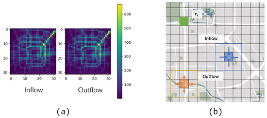
Inflow and Outflow. The traffic flow data associated with each region are the inflow and outflow, which correspond to the traffic flow entering the region from other regions and moving from the region to other regions at time t, respectively, and can be expressed as follows:

$$x_t\in R^{H\times W\times 2},$$

(1)

where $x_t^{i,j,0}and x_t^{i,j,1}$ represent the traffic flow from region $r_{i,j}$ into other regions and from other regions into $r_{i,j}$ at time interval t. The visualization is shown in Figure 2.

Figure 2. Visualization of inflow and outflow. (a) Inflow and outflow for a given time interval in the BJTaxi dataset. (b) Inflow and outflow to single areas of the city.

Definition 3. 

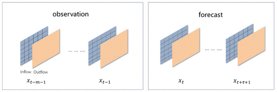
Traffic flow prediction given a sequence of historically observed traffic flow data $\{x_{t-1},\dots ,x_{t-m-1}\}$ from moment $t-1$ to moment $t-m-1$, predict the future traffic flow data $\{x_{t+1},\dots ,x_{t+1+\tau }\}$ from moment $t+1$ to moment $t+1+\tau$. The visualization is shown in Figure 3.

Figure 3. Visualization of traffic flow prediction.

3.2. Convolutional Neural Network

A Convolutional Neural Network (CNN) is a type of deep learning model that is mainly used for processing and analyzing data with a grid structure, such as images and videos. The core operation in Convolutional Neural Networks is the convolutional operation, which extracts features by sliding learnable convolutional kernels over the input data. Each convolution kernel acts as a local filter that recognizes and captures specific patterns or features at different locations in the input data. Convolutional operations exhibit weight sharing, where the same convolutional kernel shares parameters across the entire input. This property reduces the number of parameters in the model and improves generalization.

3.3. Convolutional Long Short-Term Memory

Convolutional Long Short-Term Memory (ConvLSTM) is a neural network structure based on Long Short-Term Memory (LSTM) networks, which introduces the convolutional operation in convolutional neural networks into the memory units and gating mechanisms of LSTM in order to efficiently capture spatio-temporal relationships in sequence data. ConvLSTM combines the features of CNNs and LSTM and performs well for sequential data, especially for processing video sequences or spatio-temporal sequential data. The main formulas within ConvLSTM are as follows:

$$i_t=\sigma \left(W_{xi}\ast {\mathcal{X}}_t+W_{hi}\ast {\mathcal{H}}_{t-1}+W_{ci}\circ {\mathcal{C}}_{t-1}+b_i\right)$$

(2)

$$f_t=\sigma \left(W_{xf}\ast {\mathcal{X}}_t+W_{hf}\ast {\mathcal{H}}_{t-1}+W_{cf}\circ {\mathcal{C}}_{t-1}+b_f\right)$$

(3)

$${\mathcal{C}}_t=f_t\circ {\mathcal{C}}_{t-1}+i_t\circ tanh\left(W_{xc}\ast {\mathcal{X}}_t+W_{hc}\ast {\mathcal{H}}_{t-1}+b_c\right)$$

(4)

$$o_t=\sigma \left(W_{xo}\ast {\mathcal{X}}_t+W_{ho}\ast {\mathcal{H}}_{t-1}+W_{co}\circ {\mathcal{C}}_t+b_o\right)$$

(5)

$${\mathcal{H}}_t=o_t\circ tanh\left({\mathcal{C}}_t\right)$$

(6)

where W denotes a learnable parameter; H denotes a short-term memory unit; C denotes a long-term memory unit; i, f, and o denote the input, forgetting, and output signals, respectively; ‘∗’ denotes performing a convolution operation; and ‘∘’ denotes the Hardman product.

4. Methods

In this section, we describe our model in detail. The structure of our model is shown in Figure 4. Our model is based on the Encode-Forecast structure in [23], which consists of two main parts: the Encode part for feature extraction of past traffic flow patterns at different scales, and the Forecast part for predicting future traffic flows.

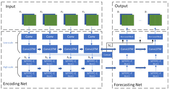
Figure 4. The multi-scale non-local spatio-temporal information fusion network (MN-STFN) framwork.

4.1. Encoding Net for Traffic Flow Pattern

The encoding part is mainly used to capture the traffic flow patterns at different scales in the past, which is divided into two parts: low-scale and high-scale. The low-scale part extracts simple traffic pattern features from the original input region, while the high-scale part enhances the input feature scale through region-wide enhancement and feature fusion to extract spatio-temporal traffic flow patterns existing in the urban region at that scale.

Firstly, the low-scale traffic flow pattern encoding (LS-E) for the input past traffic flow data sequence $X=\{x_{t-1},\dots ,x_{t-m-1}\}$ enhances the dimensionality of the traffic flow information through a convolutional network with a convolutional kernel of $1\ast 1$, and then the traffic flow information at the low scale is modeled by patterns in the temporal and spatial scales. The specific representation is as follows:

$$(h_{t_1},{\mathcal{H}}_l)=LS\text{-}E\left(x\right),$$

(7)

$$x_{\tau }^{*}=Conv\left(x_{\tau }\right),$$

(8)

$$h_{\tau +1}=ConvLSTM(x_{\tau }^{*},h_{\tau }),$$

(9)

where $x_{\tau }\in X$ denotes the initial input data at moment $\tau$, $\tau \in \{t-1,\cdots ,t-m-1\}$, ${\mathcal{H}}_l$ denotes the set of hidden states output by $ConvLSTM(•)$ at each moment in the past, $x_{\tau }^{*}$ denotes the output after dimensionality enhancement, and $h_{\tau }$ denotes the hidden state at moment $\tau$.

This is immediately followed by the high-scale traffic flow model encoding (HS-E), which consists of several constantly overlapping MTFPC-E blocks, the structure of which is shown in Figure 5. The upper part indicates the internal structure of the MTFPC-E, while the lower part indicates the variation in the regional scale.

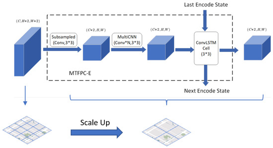
Figure 5. Multi-scale Traffic Flow Pattern Capture block for encoding (MTFPC-E).

The input for a single MTFPC-E block is the traffic pattern coding result from the LS-E or the output of the previous MTFPC-E block. The downsampling process begins with a convolutional layer that uses a $3\ast 3$ kernel to reduce the scale of the input tensor by half. This allows for the fusion of traffic flow features between neighboring regions and the combination of multiple neighboring regions into a single one, resulting in an expanded region range. To minimize the loss of traffic information during the fusion process, the final output region features will be doubled in dimension when downsampling is performed. Following this, a multilayer convolutional network extracts traffic flow features between regions in a larger scale space. Finally, the traffic flow features are extracted over time using ConvLSTM combined with the traffic features from the same scale in the previous moment. The final output is the traffic flow pattern code at that scale. The code can be expressed as follows:

$$h_t^s=MTFPC\text{-}{E}_s(h_t^{s-1},h_s^{t-1}),$$

(10)

where s denotes the current number of layers of $MTFPC\text{-}E$, s denotes the current moment, $h_t^s$ denotes the coded output at moment t in this scale, and $h_{t-1}^s$ denotes the hidden state at the previous moment.

By flexibly adjusting the number of layers and the number of stacks of convolutional layers in the MTFPC-E block, it is possible to realize the capture of the unique traffic flow pattern characteristics at different scales. However, it should be noted that in order to achieve the best performance of the model, it should be ensured that the total convolutional sensory fields of both LS-E and HS-E are similar to the scale of the original input data.

4.2. Forecasting Net

The forecasting part is used for forecasting and scale reduction in the input hidden state of the previous moment, and the beginning part of its structure is similar to the coding structure, which is also divided into high-scale prediction reduction (HS-F) and low-scale prediction reduction (LS-F). For a given moment, the first part is the high-scale prediction reduction, which is realized by the constantly stacked MTFPC-F block:

$$y_t^{s-1}=MTFPC\text{-}{F}_s(y_t^s,h_{t-1}^s)$$

(11)

where s denotes the current number of layers of the $MTFPC\text{-}F$ block; t denotes the current moment; $y_t^s$ denotes the input at this scale, which can also be regarded as the predicted reduced output of the previous scale; $h_{t-1}^s$ denotes the state of the predicted predicted output of the previous moment, which serves as the starting input for the prediction; and $y_t^s$ will be set to an all-zero tensor.

The structure of the MTFPC-F block is shown in Figure 6, where the upper half indicates the internal structure of MTFPC-F and the lower half indicates the variation in the regional scale. For the input prediction results of the previous scale, the ConvLSTM is first used to predict the traffic flow characteristics of the previous moment in time, and then the predicted inputs are spatially reduced by a multilayer inverse convolutional network, and finally the predicted outputs are scaled by an inverse convolutional network with a convolutional kernel of $3\ast 3$.

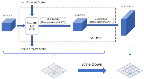
Figure 6. Multi-scale Traffic Flow Pattern Capture block for forecasting (MTFPC-F).

LS-F follows HS-F, which makes low-scale predictions based on high-scale outputs. Its structure consists of ConvLSTM with a non-local block, which can be represented as follows:

$$Y=LS\text{-}F(Y_l,H_l)$$

(12)

$$y_t^{*}=ConvLSTM(y_t^1,h_t^1)$$

(13)

$$y_t=Non\text{-}Local(y_t^{*},{\mathcal{H}}_l)$$

(14)

where $Y_t$ denotes the set of predicted outputs at the high scale and Y denotes the final prediction result. For the inputs with the previous scale, the prediction is firstly corrected by ConvLSTM at the low scale, and then the final and prediction results are outputted by establishing a direct connection between the past hidden state and the current prediction inputs according to the non-local block, which will be introduced in the next section.

4.3. Non-Local Block

Non-local networks [28], a network structure mainly applied in computer vision, establish the dependency between a local point and all other points by computing the similarity between global and local features. Although deep convolutional networks can provide a large enough receptive field to capture the global change pattern of features, this method is computationally intensive and inefficient, and it is difficult to establish the connection of long-distance local features through the superposition of convolutional kernels or recurrent neural networks. The idea of non-local is to break through the limitation of the receptive field of the network and directly establish long-distance dependency relationships between different time slices of points and points. In traffic flow information, a dense traffic area in the initial time slice will affect the traffic flow in other key areas of the city in the future after spreading over many moments. The introduction of a non-local block in the initial stage of local spatio-temporal feature extraction will help the network to capture the spatial and temporal connections between localized areas of the city and improve the accuracy of the model prediction.

The original network structure in [28] establishes a corresponding relationship within a tensor, between local features and global features. In contrast, our non-local block establishes a long-distance dependency between the low-scale prediction outputs and the set of hidden states output from past low-scale ConvLSTM.

Figure 7 shows the internal structure of our non-local block, which $\mathcal{H}$ represents the set of low-scale traffic flow features at different moments in the encoding part, $y_t^{*}$ represents the low-scale traffic prediction results in the prediction part, $\varphi$ and $\mu$ represent two convolutional networks with kernel sizes of $1\ast 1$ and $1\ast 1\ast 1$, respectively, which are used to reduce the dimensionality of the input features to reduce the amount of computation. After the two convolutional networks, the influence relationship between regions can be represented by a dot product, and the region relationship matrix A can be calculated by matrix multiplication:

$$A=\varphi \left(Y_t^{*}\right)\mu \left({\mathcal{H}}_l\right),$$

(15)

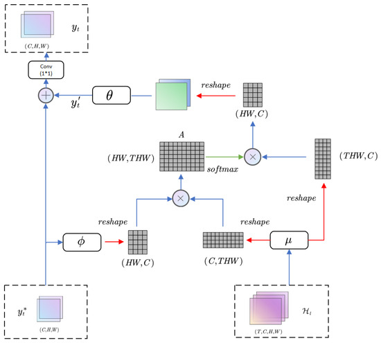
Figure 7. The structure of non-local block.

After normalizing the relationship matrix A, the low-scale traffic flow feature tensor after dimensionality reduction is multiplied to obtain the influence values of all regions in the past on the current prediction region. The feature dimensionality is then reduced by a convolutional network with a $1\ast 1$ convolutional kernel and added back to the original low-scale traffic prediction to obtain the final prediction. Similar to the encoding in the initial input section where the dimension of the traffic flow information is increased for individual regions, the dimension of the prediction result is reduced again by a convolutional network to the same dimension as the validation tensor before the final output of the block:

$$y_t^{\prime }=softmax\left(A\right)\mu \left({\mathcal{H}}_l\right),$$

(16)

$$y_t=Conv(y_t^{*}+y_t^{\prime })$$

(17)

5. Experiments

5.1. Datasets

We use two publicly available real-world datasets [3], BJTaxi and NYCBike, to train and compare the performance of the models, as shown in Table 1. The details of the datasets are given as follows:

Table 1. Statistics for Datasets.

Datasets	Time Interval	Taxis/Bikes	Regions	Available Time Interval	Data Type
BJTaxi	30 min	34k+	32 × 32	22,459	Taxi GPS
NYCBike	1 h	6.8k+	16 × 8	4392	Bike rent

• BJTaxi: The dataset was collected from the real GPS movement trajectories of Beijing cabs from 2013–2016, which are processed and divided into $32\ast 32$ specification grid data, and a single grid contains both inflow and outflow features, and the whole dataset is divided into data at 30-min intervals, and the number of available time intervals is 22,459. We use the last four weeks of data as test data and all the rest of the data are used for training.
• NYCBike: This dataset was collected with the movement trajectories of New York public bicycles from April 2014 to September 2014. The grid size of the region is $16\ast 9$, the time interval of data collection is one hour, and the available time interval is 4392; we use the data of the last 10 days as the test data, and the rest of the data are used as the training data.

Before using the data, we processed the data in a uniform manner. The raw data are processed as regular grid data in [3]. Similarly to [19], to maintain data continuity, for dates with missing data, all data within that day are removed. Individual data are a continuous time series and the next data are obtained by jumping individual time intervals. Next, Min-Max Normalization is performed on all data prior to training to scale the data to between $[0,1]$, and then the data are reduced back to their original size when error validation is performed.

5.2. Baselines

Our model will be compared to the following seven benchmark models.

• SVR: Support Vector Regression (SVR) is an application of Support Vector Machines (SVMs) to solve regression problems. Unlike traditional linear regression models, SVR can handle non-linear relationships and is very effective in dealing with high-dimensional data and noise in data.
• LSTM: It is a variant of recurrent neural networks (RNNs) for processing and modeling time series data and other sequence data with temporal dependencies. LSTM is designed to solve the problem of gradient vanishing in traditional RNNs to better capture long-term dependencies.
• ST-SSL [14]: It proposes a novel spatio-temporal self-supervised learning traffic prediction framework, a spatio-temporal convolutional module on top of a complementary self-supervised learning paradigm to enhance traffic pattern representation and identify spatial and temporal heterogeneity in traffic flows. Due to model structural limitations, only single-step prediction performance is compared for this model.
• ConvLSTM [23]: Its combining of convolutional networks with LSTM allows it to capture the existence of local dependencies in spatio-temporal data.
• SA-ConvLSTM [17]: A variant of ConvLSTM to capture long-term dependencies in the presence of time series by introducing self-attention as well as additional memory units.
• ST-ResNet [3]: It is a traffic flow prediction model based on deep residual networks. By stacking residual units, three different cycles of traffic flow data are processed separately to capture the spatio-temporal correlations present in the traffic data.
• AttConvLSTM [19]: It is a multi-step traffic flow prediction model based on sequence-to-sequence architecture, which establishes the influence relationship between regions at a long distance by introducing an attention mechanism to the hidden states at different moments.

The source code of our model is released on GitHub (https://github.com/RicardeLu/MN-STFN, accessed 18 December 2023).

5.3. Evaluation Metrics and Settings

We use root mean square error (RMSE) and mean absolute percentage error (MAPE) as the evaluation function for performance comparison, which is defined as follows:

$$RMSE=\sqrt{\frac{1}{n}\sum _{i=1}^n{({\widehat{y}}_i-y_i)}^2}$$

(18)

$$MAPE=\frac{100\%}{n}\sum _{i=1}^n\left|\frac{{\widehat{y}}_i-y_i}{y_i}\right|$$

(19)

Our model was implemented using Pytorch, with the number of model training rounds set to 200, batchsize set to 32, and model optimization using Adam [29], with the learning rate set to 0.001 and exponential decay of the learning rate set to 0.995. All convolutional kernels within the model were set to 3, and the model was trained using a single NVIDIA 3080ti.

5.4. Comparing with Baselines

Table 2 and Table 3 show the evaluation results of all models on the BJTaxi dataset. Table 4 and Table 5 demonstrate the evaluation results of all models on the NYCBike dataset. On the BJTaxi dataset, the number of CNN layers inside the MTFPC block of the model is set to 4 and the number of blocks is set to 2. On the NYCBike dataset, the number of internal CNN layers is set to 2 and the number of blocks is set to 1. Figure 8 and Figure 9 show the trend of the prediction performance of the main models on the BJTaxi dataset and the NYCBike dataset. From these graphs, we can make the following observations:

Table 2. The RMSE results for BJTaxi dataset.

Methods	RMSE of $\mathit{\tau }$ Step Prediction
	1	2	3	4	5
SVR	39.26	44.49	48.51	51.79	54.38
LSTM	16.21	18.49	19.25	20.02	20.85
ST-SSL	17.82	-	-	-	-
ConvLSTM	17.46	21.19	24.10	26.39	29.23
SA-ConvLSTM	15.66	16.35	17.28	17.78	18.38
ST-ResNet	16.42	17.80	18.65	19.35	19.77
AttConvLSTM	19.11	19.68	22.32	24.81	26.87
MN-STFN	14.13	15.54	16.35	17.67	17.95

The best result in each prediction step is indicated in bold.

Table 3. The MAPE results for BJTaxi dataset.

Methods	MAPE of $\mathit{\tau }$ Step Prediction
	1	2	3	4	5
SVR	0.4281	0.4409	0.4499	0.4568	0.4626
LSTM	0.3661	0.3973	0.4020	0.4336	0.4384
ST-SSL	0.2196	-	-	-	-
ConvLSTM	0.2940	0.3599	0.4151	0.4742	0.5481
SA-ConvLSTM	0.2294	0.2322	0.2419	0.2436	0.2505
ST-ResNet	0.2252	0.2381	0.2455	0.2563	0.2586
AttConvLSTM	0.3727	0.4022	0.4676	0.5510	0.5660
MN-STFN	0.2081	0.2294	0.2354	0.2420	0.2464

The best result in each prediction step is indicated in bold.

Table 4. The RMSE results for NYCBike dataset.

Methods	RMSE of $\mathit{\tau }$ Step Prediction
	1	2	3	4	5
SVR	10.75	12.61	13.86	14.57	16.79
LSTM	4.85	5.74	5.62	6.08	6.71
ST-SSL	4.62	-	-	-	-
ConvLSTM	5.65	7.25	8.41	9.29	9.55
SA-ConvLSTM	4.68	5.22	5.62	6.08	6.71
ST-ResNet	4.51	5.03	5.49	6.07	6.54
AttConvLSTM	4.89	5.76	6.15	6.70	7.41
MN-STFN	4.49	5.08	5.50	5.93	6.68

The best result in each prediction step is indicated in bold.

Table 5. The MAPE results for NYCBike dataset.

Methods	MAPE of $\mathit{\tau }$ Step Prediction
	1	2	3	4	5
SVR	0.5832	0.6489	0.6959	0.5993	0.6136
LSTM	0.4370	0.4917	0.5510	0.5677	0.6345
ST-SSL	0.3018	-	-	-	-
ConvLSTM	0.5025	0.6021	0.6472	0.6482	0.6793
SA-ConvLSTM	0.4072	0.4153	0.4303	0.4415	0.4860
ST-ResNet	0.3920	0.4396	0.4624	0.4772	0.5023
AttConvLSTM	0.4321	0.4576	0.4728	0.5058	0.5729
MN-STFN	0.3895	0.4082	0.4286	0.4322	0.4848

The best result in each prediction step is indicated in bold.

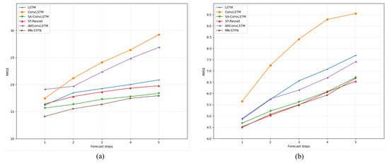
Figure 8. Comparison of RMSE results for several major models. (a) BJTaxi. (b) NYCBike.

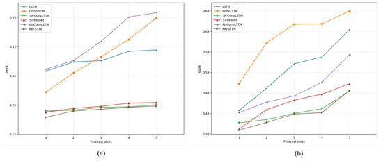
Figure 9. Comparison of MAPE results for several major models. (a) BJTaxi. (b) NYCBike.

• On the BJTaxi dataset, our model (MN-STFN) shows better performance compared to other existing methods. We are the first model to reduce the RMSE to below 15 on single-step prediction, which shows that our non-local network with multi-scale traffic pattern capture can effectively reduce the prediction error of the model; on the 2–5-step prediction, the performance is constantly leaning towards SA-ConvLSTM but it still manages to achieve the minimum error on multi-step prediction. Our model also has the lowest error on MAPE, outperforming all other models in both single-step and multi-step prediction.
• For the results on the NYCBike dataset, our model shows better performance in RMSE compared to the rest of the models for 1–4 step prediction, while ST-ResNet shows better performance for 5-step prediction. As for the results on MAPE, ST-SSL shows better performance in the case of single-step prediction; while in the case of multi-step prediction, our model performs better than the rest of the models.
• With the exception of ST-SSL, which shows better performance on the single-step prediction of MAPE results, the difference in the performance of all models on the NYCBike dataset is not as pronounced as on the BJTaxi dataset. The reason may be that the total data volume of the NYCBike dataset is much smaller than that of the former, the difference in traffic flow variations in the dataset is not very large, the traffic flow patterns in the data are relatively simple, and the existing methods are able to capture the flow patterns that exist in them well. Therefore, except for SVR, the performance difference in the other models in this dataset is not very obvious. On the other hand, the NYCBike dataset area is not very large, and thus its flow patterns do not vary much at different scales, which makes our multi-scale structure not work well. Nevertheless, the prediction results of our model on the NYCBike dataset are still able to approach and exceed the best existing models, and with the expansion of the prediction area, our model is able to better capture the complex traffic flow patterns and show excellent prediction performance.

Figure 10 demonstrates the comparison of the predicted values of our model with ground truth data under the BJTaxi dataset in the case of single-step prediction. It can be observed that our model can capture the cyclical pattern of regional traffic flow changes well, and for short-term traffic flow changes, the model can also fit the trend of traffic flow changes.

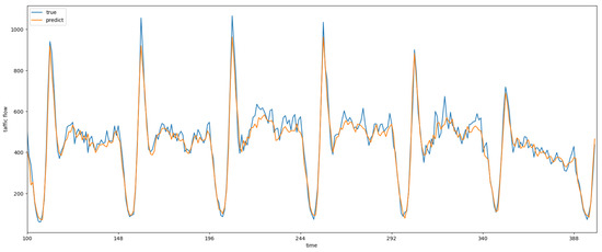
Figure 10. Single-step forecast scenario for individual area traffic flow predictions compared to true values.

5.5. Effect of Multi-Scale Traffic Flow Pattern Capture

By evaluating the performance of our model under different block layer stacks, we are able to show how well our model captures traffic flow patterns at different scales. In the validation, the number of convolutional layers in the block is uniformly set to 4, and the number of prediction steps is set to 1, 3 and 5, respectively; more layers stacked in the block indicates the capture of traffic flow patterns at higher scales. Table 6 demonstrates the comparison of the performance under multi-step prediction for models with different numbers of blocks under the BJTaxi dataset. We can observe that along with the stacking of blocks, the single-step prediction error of the model decreases and then increases, and the model reaches the best performance at block number 2.

Table 6. Effect of Multi-scale Traffic Flow Pattern Capture in BJTaxi dataset.

Block Number	RMSE of $\mathit{\tau }$ Step Prediction
	1	3	5
MTFPC-1	14.21	16.42	17.82
MTFPC-2	14.13	16.35	17.95
MTFPC-3	14.41	16.62	17.96

The best result in each prediction step is indicated in bold.

To further verify the effect of traffic flow patterns on the prediction results at different scales, we visualize the prediction error of a sample in the BJTaxi dataset under two different mode scale models. The visualization results are shown in Figure 11.

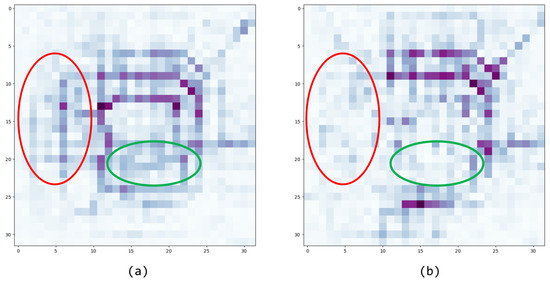
Figure 11. Visualization of errors in single-step prediction results for different scale models. The prediction error in a region increases as the color of the region gets darker. (a) MTFPC-1. (b) MTFPC-2.

It can be observed that the model that can capture the high-scale information has a lower error compared to the low scale model in the area marked in Figure 11.

5.6. Effect of Low-Scale Hidden-State Dimensions

The model embeds the features of the original high-dimensional input data into the low-scale traffic flow feature extraction part. The size of the hidden state of the low-scale traffic flow pattern affects the size of the feature extraction of the high-scale traffic flow pattern, which in turn affects the size of the capacity of the whole model. To demonstrate the effect of different low-scale hidden-state dimensions on the model performance, we evaluated three different models with low-scale dimensions of 8, 16, and 32. Table 7 and Figure 12 show the performance comparison of the three models for multi-stage prediction on the BJTaxi dataset. We can observe the low-scale hidden-state dimension of 16. At 8 and 32, the model is underfitting and overfitting, respectively.

Table 7. Comparison of predictive performance of models with different hidden dimensions.

Input Dim	RMSE of $\mathit{\tau }$ Step Prediction
	1	3	5
8	14.48	17.26	18.87
16	14.13	16.35	17.95
32	14.67	16.52	17.99

The best result in each prediction step is indicated in bold.

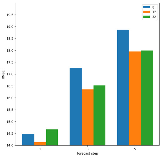
Figure 12. The visualization comparison of the predictive performance of models with different hidden dimensions.

5.7. Effect of Non-Local Block

Our non-local block is used to establish a spatio-temporal connection between the prediction tensor and past hidden states. The role of the non-local structure for establishing direct spatio-temporal dependencies between local regions and the global region is assessed by performing ablation experiments on it. We perform ablation studies by carefully designing the following variant.

• MN-STFN-dc: It uses an transposed convolution layer instead of a non-local block to transform the hidden state dimension into the predicted output dimension.

The forecasting performance of the two models on the BJTaxi dataset is shown in Table 8. It can be observed that our non-local block can effectively reduce the forecasting error of the model and improve the performance of the model, both in single-step forecasting and multi-step forecasting.

Table 8. Effect of non-local block on BJTaxi dataset.

Methods	RMSE of $\mathit{\tau }$ Step Prediction
	1	3	5
MN-STFN-dc	14.32	16.75	18.32
MN-STFN	14.13	16.35	17.95

The best result in each prediction step is indicated in bold.

To visualize more intuitively the effect of the non-local networks on the model, we compare the prediction errors of the two models for a single step in Figure 13. It can be clearly observed that for the model without non-local networks, the prediction errors are distributed around all the traffic flow routes, while on the contrary, for the added model, the errors shrink to the vicinity of the main roads where the urban traffic flows rapidly. Figure 14 shows a heat map of the influence of past moments on the prediction results of individual grids, and from the markers in the figure, it can be observed that the network tends to establish the connection between individual areas and important traffic nodes for the more recent observations, while as the time span increases, the network instead decreases this hotspot-region connection and tends to establish a single-region global connection. This further demonstrates the effectiveness of our non-local networks for establishing global dependencies.

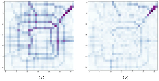
Figure 13. Visualization of the error of single-step and prediction results for two models with a single sample. The prediction error in a region increases as the color of the region gets darker. (a) MN-STFN-dc. (b) MN-STFN.

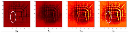
Figure 14. Visualization of the influence of input data on individual grids in the prediction results.

6. Conclusions

In this paper, we propose a multi-scale non-local spatio-temporal information fusion network (MN-STFN) for multi-step prediction of traffic flow. The extraction of spatio-temporal flow features of traffic flow at different scales is realized by stacking multiple multi-scale traffic flow pattern capture (MTFPC) blocks, and supplemented with a non-local network to capture direct spatio-temporal dependencies between local regions and the global region to improve the accuracy of prediction. The performance evaluation results for the BJTaxi dataset and the NYCBike dataset show that our model exhibits better performance on the multi-step prediction of traffic flow compared to the benchmark model. The evaluation comparison for these two datasets of different magnitudes also shows that our model is able to comprehensively capture and predict the simple traffic flow model for smaller regions, while along with the increase in the prediction region, our model is able to show better performance in modeling regional relationships and predicting future traffic flow compared to other models. We also verify the effectiveness of the MTFPC block and non-local block by comparing a series of ablation experiments. The multi-scale structure will help the model to more comprehensively construct the complex traffic flow patterns existing in the city, rather than local modules, and intuitively show the impact of the historical traffic flow changes on the current moment, which will help city managers to more comprehensively grasp the current state of urban traffic flow and make the right decision for future urban planning in combination with real needs.

In our future work, we will explore the following directions: first, improve the model structure to reduce the impact on the accuracy of multi-step prediction due to error accumulation and achieve longer-term traffic flow prediction, and second, consider the impact of additional factors such as weather and holidays in the prediction to reduce uncertainty in the model prediction.

References

- Zheng, Y.; Capra, L.; Wolfson, O.; Yang, H. Urban computing: Concepts, methodologies, and applications. ACM Trans. Intell. Syst. Technol. TIST 2014, 5, 1–55. [Google Scholar] [CrossRef]
- Zhang, J.; Zheng, Y.; Qi, D.; Li, R.; Yi, X. DNN-based prediction model for spatio-temporal data. In Proceedings of the 24th ACM SIGSPATIAL International Conference on Advances in Geographic Information Systems, Burlingame, CA, USA, 31 October–3 November 2016; pp. 1–4. [Google Scholar]
- Zhang, J.; Zheng, Y.; Qi, D. Deep spatio-temporal residual networks for citywide crowd flows prediction. In Proceedings of the AAAI Conference on Artificial Intelligence, San Francisco, CA, USA, 4–9 February 2017; Volume 31. [Google Scholar]
- Chen, Q.; Song, X.; Yamada, H.; Shibasaki, R. Learning deep representation from big and heterogeneous data for traffic accident inference. In Proceedings of the AAAI Conference on Artificial Intelligence, Phoenix, AZ, USA, 12–17 February 2016; Volume 30. [Google Scholar]
- Jayarajah, K.; Tan, A.; Misra, A. Understanding the Interdependency of Land Use and Mobility for Urban Planning. In Proceedings of the the 2018 ACM International Joint Conference and 2018 International Symposium, Singapore, 8–12 October 2018. [Google Scholar]
- Wang, Y.; Tong, D.; Li, W.; Liu, Y. Optimizing the spatial relocation of hospitals to reduce urban traffic congestion: A case study of Beijing. Trans. GIS 2019, 23, 365–386. [Google Scholar] [CrossRef]
- Chen, Y.; Wu, G.; Chen, Y.; Xia, Z. Spatial Location Optimization of Fire Stations with Traffic Status and Urban Functional Areas. Appl. Spat. Anal. Policy 2023, 16, 771–788. [Google Scholar] [CrossRef]
- Ali, A.; Terada, K. A framework for human tracking using kalman filter and fast mean shift algorithms. In Proceedings of the 2009 IEEE 12th International Conference on Computer Vision Workshops, ICCV Workshops, Kyoto, Japan, 27 September–4 October 2009; pp. 1028–1033. [Google Scholar]
- Kumar, S.V.; Vanajakshi, L. Short-term traffic flow prediction using seasonal ARIMA model with limited input data. Eur. Transp. Res. Rev. 2015, 7, 21. [Google Scholar] [CrossRef]
- Zheng, J.; Ni, L.M. An unsupervised framework for sensing individual and cluster behavior patterns from human mobile data. In Proceedings of the 2012 ACM Conference on Ubiquitous Computing, Pittsburgh, PA, USA, 5–8 September 2012; pp. 153–162. [Google Scholar]
- Ye, Y.; Zheng, Y.; Chen, Y.; Feng, J.; Xie, X. Mining individual life pattern based on location history. In Proceedings of the 2009 Tenth International Conference on Mobile Data Management: Systems, Services and Middleware, Washington, DC, USA, 18–20 May 2009; pp. 1–10. [Google Scholar]
- Fu, X.; Yu, G.; Liu, Z. Spatial–temporal convolutional model for urban crowd density prediction based on mobile-phone signaling data. IEEE Trans. Intell. Transp. Syst. 2021, 23, 14661–14673. [Google Scholar] [CrossRef]
- Yu, B.; Yin, H.; Zhu, Z. Spatio-temporal graph convolutional networks: A deep learning framework for traffic forecasting. arXiv 2017, arXiv:1709.04875. [Google Scholar]
- Ji, J.; Wang, J.; Huang, C.; Wu, J.; Xu, B.; Wu, Z.; Zhang, J.; Zheng, Y. Spatio-temporal self-supervised learning for traffic flow prediction. In Proceedings of the AAAI Conference on Artificial Intelligence, Washington, DC, USA, 7–14 February 2023; Volume 37, pp. 4356–4364. [Google Scholar]
- Zhou, Z.; Wang, Y.; Xie, X.; Qiao, L.; Li, Y. STUaNet: Understanding uncertainty in spatiotemporal collective human mobility. In Proceedings of the Web Conference 2021, Ljubljana, Slovenia, 19–23 April 2021; pp. 1868–1879. [Google Scholar]
- Zhang, Y.; Li, Y.; Zhou, X.; Luo, J.; Zhang, Z.L. Urban traffic dynamics prediction—a continuous spatial-temporal meta-learning approach. ACM Trans. Intell. Syst. Technol. TIST 2022, 13, 1–19. [Google Scholar] [CrossRef]
- Lin, Z.; Li, M.; Zheng, Z.; Cheng, Y.; Yuan, C. Self-attention convlstm for spatiotemporal prediction. In Proceedings of the AAAI Conference on Artificial Intelligence, New York, NY, USA, 7–12 February 2020; Volume 34, pp. 11531–11538. [Google Scholar]
- Wang, D.; Yang, Y.; Ning, S. DeepSTCL: A deep spatio-temporal ConvLSTM for travel demand prediction. In Proceedings of the 2018 International Joint Conference on Neural Networks (IJCNN), Rio de Janeiro, Brazil, 8–13 July 2018; pp. 1–8. [Google Scholar]
- Liu, C.H.; Piao, C.; Ma, X.; Yuan, Y.; Tang, J.; Wang, G.; Leung, K.K. Modeling citywide crowd flows using attentive convolutional lstm. In Proceedings of the 2021 IEEE 37th International Conference on Data Engineering (ICDE), Chania, Greece, 19–22 April 2021; pp. 217–228. [Google Scholar]
- Zheng, H.; Lin, F.; Feng, X.; Chen, Y. A hybrid deep learning model with attention-based conv-LSTM networks for short-term traffic flow prediction. IEEE Trans. Intell. Transp. Syst. 2020, 22, 6910–6920. [Google Scholar] [CrossRef]
- Li, Z.; Han, Y.; Xu, Z.; Zhang, Z.; Sun, Z.; Chen, G. PMGCN: Progressive Multi-Graph Convolutional Network for Traffic Forecasting. ISPRS Int. J. Geo-Inf. 2023, 12, 241. [Google Scholar] [CrossRef]
- Li, Y.; Yu, R.; Shahabi, C.; Liu, Y. Diffusion convolutional recurrent neural network: Data-driven traffic forecasting. arXiv 2017, arXiv:1707.01926. [Google Scholar]
- Shi, X.; Chen, Z.; Wang, H.; Yeung, D.Y.; Wong, W.K.; Woo, W.C. Convolutional LSTM network: A machine learning approach for precipitation nowcasting. Adv. Neural Inf. Process. Syst. 2015, 28, 802–810. [Google Scholar]
- Pan, Z.; Liang, Y.; Wang, W.; Yu, Y.; Zheng, Y.; Zhang, J. Urban traffic prediction from spatio-temporal data using deep meta learning. In Proceedings of the 25th ACM SIGKDD International Conference on Knowledge Discovery & Data Mining, Anchorage, AK, USA, 4–8 August 2019; pp. 1720–1730. [Google Scholar]
- Pan, Z.; Ke, S.; Yang, X.; Liang, Y.; Yu, Y.; Zhang, J.; Zheng, Y. AutoSTG: Neural Architecture Search for Predictions of Spatio-Temporal Graph. In Proceedings of the Web Conference 2021, Ljubljana, Slovenia, 19–23 April 2021; pp. 1846–1855. [Google Scholar]
- Vaswani, A.; Shazeer, N.; Parmar, N.; Uszkoreit, J.; Jones, L.; Gomez, A.N.; Kaiser, Ł.; Polosukhin, I. Attention is all you need. Adv. Neural Inf. Process. Syst. 2017, 30, 6000–6010. [Google Scholar]
- Liu, L.; Zhang, R.; Peng, J.; Li, G.; Du, B.; Lin, L. Attentive crowd flow machines. In Proceedings of the 26th ACM international conference on Multimedia, Seoul, Republic of Korea, 22–26 October 2018; pp. 1553–1561. [Google Scholar]
- Wang, X.; Girshick, R.; Gupta, A.; He, K. Non-local neural networks. In Proceedings of the IEEE Conference on Computer Vision and Pattern Recognition, Salt Lake City, UT, USA, 18–22 June 2018; pp. 7794–7803. [Google Scholar]
- Kingma, D.P.; Ba, J. Adam: A method for stochastic optimization. arXiv 2014, arXiv:1412.6980. [Google Scholar]
Disclaimer/Publisher’s Note: The statements, opinions and data contained in all publications are solely those of the individual author(s) and contributor(s) and not of MDPI and/or the editor(s). MDPI and/or the editor(s) disclaim responsibility for any injury to people or property resulting from any ideas, methods, instructions or products referred to in the content. |
© 2024 by the authors. Licensee MDPI, Basel, Switzerland. This article is an open access article distributed under the terms and conditions of the Creative Commons Attribution (CC BY) license (https://creativecommons.org/licenses/by/4.0/).