Article

Uncovering Factors Affecting Taxi Income from GPS Traces at the Directional Road Segment Level

1
School of Intelligent Systems Engineering, Sun Yat-sen University, Shenzhen 518107, China
2
School of Civil Engineering, Tsinghua University, Beijing 100084, China
3
School of Art and Design, Xi’an University of Technology, Xi’an 710061, China
4
Department of Civil and Environmental Engineering, Nagoya University, Nagoya 464-8603, Japan
*
Author to whom correspondence should be addressed.
ISPRS Int. J. Geo-Inf. 2022, 11(8), 431; https://doi.org/10.3390/ijgi11080431
Submission received: 6 June 2022 / Revised: 21 July 2022 / Accepted: 26 July 2022 / Published: 31 July 2022

Abstract

:
Nowadays, the market demand for taxis is still intense. However, there exist lots of issues affecting the healthy development of the taxi industry, such as an increasing difficulty in hailing taxis, detouring behavior etc., and especially, the low incomes of taxi drivers. This paper establishes a multi-layer road index (MRI) system of 7862 directional road segments (DRSs), and collects over 194 million occupied GPS points within a week, revealing the factors affecting taxi drivers’ incomes in Shenzhen, China. The income differences has been identified on different DRSs, which accordingly have been categorized into two levels. Four categories of DRS factors, i.e., road attributes, traffic dynamics, points of interest (POIs), and taxi operation strategies, are defined as the impact factors affecting income levels. The selected sample-based binomial logit (SBL) model has been proposed to reveal the significance of these influencing factors. The results indicate that the road segments with different features have different incomes over different time periods. The main factors in income analysis are the factors used to represent taxi operation strategies. Highly rewarding pick-up road segments can be identified, which could contribute to drivers’ income improvements, and can further contribute to the development of the taxi market.

1. Introduction

Taxis play an important role in public transportation provision—effectively plugging the gaps that are left by buses and subways. Generally, they are not considered to be a luxury mode of transport—they are predominantly used by people with mobility problems, and by people who do not own cars, to perform trips that would have otherwise been impossible. As for Shenzhen, in 2015, it has been recorded that there were 16,597 taxis delivering more than 1.1 million passengers per day, which constitute an indispensable part of the city’s traffic ecosystem.
In most European countries, taxi fares include a flag-down fare, a fare charged by the ride length, a congestion premium (or so-called low-speed fare, which is the cost of waiting upon the request of the passenger), and other expenses (such as fuel surcharges) [1], which are normally regulated by the taxi associations and regulators. The entry regulation has been formulated in Belgium, Italy, France, and other countries [2]. In other countries, deregulation policies lead to a sharp increase in the number of taxis and have dramatically declined the service quality [3]. Especially with lower incomes, the drivers tend to decline in their service quality. Therefore, establishing a fair, efficient, and comprehensive fare policy and service management system is essential and critical for a boom in the global taxi industry.
For the China taxi industry, the income level is still a major concern for taxi drivers and regulators. However, with the growth of the taxi market and changes in travel demands, a lot of problems have accumulated, such as service refusal, cruising, and taxi strikes [4]. For instance, in December 2020, the Shenzhen Municipal Transportation Bureau received 71.43% of complaints against the taxi service. Since 2004, nearly 200 taxi strikes have taken place across the country, involving more than 100 cities nationwide. Especially, since 2015, taxi strikes have been spreading to the big cities, including Shenyang, Changchun, Jinan, Chengdu, and other provincial capitals. These phenomena are ultimately due to low income. Taxi drivers tend to avoid driving during peak hours, because they earn less than expected, and do not know where the high-paying areas are. Therefore, instead of being blocked in a traffic jam, drivers plan for suspension of their services, and they have a rest. In order to maximize profits, in the past few years, taxi drivers always reduce the empty rate by increasing the number of passengers, which is influenced by taxi revenue models and the hunting-cruising service method [5,6]. Nowadays, online driving services provide a new opportunity. Taxi drivers can select the destination across different online taxi service platforms. The destination plays an important role in in determining their income.
The orders of ride-hailing and incomes vary with regions and times. Experienced taxi drivers tend to have higher incomes. These drivers usually spend less time looking for new passengers, because they know where the high-income areas are, according to different time periods and regions [7,8]. Therefore, based on driving experience, they can reasonably choose the cruise route and the order destination. However, for most drivers, they do not have enough experience to determine their range of motion to maximize the average hourly income. As a result, there is an interesting phenomenon where passengers cannot find taxis and drivers cannot find passengers. The reason for this embarrassing, as the driver is blind when searching passengers while using an inefficient ride-hailing operation system [9,10].
To improve the taxi operation efficiency, it is essential to understand the distribution of passengers with high profits. Especially during peak hours, driver income is highly reduced by prolonged periods of being stuck in congestion. Although some research indicates that congestion charges will eliminate the impact of congestion, the effects may not seem like much [1]. Activity hotspots are sometimes being misused by taxi drivers to identify high-income areas, but this method may not be referenced to grasp high-driving profits, instead of the density. Therefore, this paper intends to seek the spatiotemporal distribution law of high taxi income from the inherent attributes of the road sections (including directionality, connection attributes, land use characteristics, etc.) as an initial reference for taxi drivers.
This study aims to identify the road segments of high incomes. The payment for each path is calculated to the road segment where the travel starts. Charging methods can be formulated based on the results to improve the operational efficiency of the taxi market. Further suggestions of cruising can be put up for taxi companies and drivers to increase their daily income, and to improve the efficiency of the taxi industry. The contributions of this paper are as follows: (1) The multi-layer road index (MRI) system has been used for map matching and for calculating the spatiotemporal distribution of taxi revenue in units of directional road segments. (2) A large sample of urban road sections is obtained, with the income of each direction, and the tendency of taxi income in different time periods are analyzed. (3) Except for the driver service strategy, this paper fully considers the road characteristics, with directions in impacting the taxi income.
The remainder of this article is organized as follows: Section 2 reviews the methods and factors for identifying taxi incomes; Section 3 presents the data collection methods. Section 4 illustrates the results of the high-income areas and their causes. Section 5 proposes appropriate conclusions and policy recommendations with regard to increasing the taxi incomes.

2. Literature Review

In the past two decades, research into taxi income can be classified by whether taxi GPS data is being used. On the one hand, the research is mainly focused on theoretical investigations without using GPS data. On the other hand, GPS data-based research tends to be problem-solving oriented, and is the mainstream academic research method nowadays. Previous research has evidenced that a certain intelligence lies in taxi drivers’ waiting, hunting, and cruising behaviors [11,12]. Following Castro and Gao, etc., to some extent, such behavior indicates the urban wisdom and experience possessed by taxi GPS data [13,14,15]. The mining of taxi trajectories is also widely applied in path recommendation [16,17], mobility pattern detection [18,19], spatiotemporal dynamics analysis [20,21], and congestion estimation [22] etc., nowadays. Therefore, GPS data-based income research is the trend of future works in taxi investigation.
GPS data-based research has already influenced the income of the taxi drivers. These related researches are mainly focused on revealing the crowd-intelligence of the taxi income, which are affected by the driving model [23], likelihood of pick ups [24], working time [25,26], speed changing [24,27], taxi service strategy, etc. For instance, in the research of taxi service strategy, the main aspects include space-time distribution of passenger sources [28], space-time patterns on cruising trips and stopping spots [29], hot-spot regions [30], mileage or time utilization ratio [31], and region selection [14,32,33], etc. In addition to these factors, there are also some external authors added indicators concerning as the impact factor of the taxi income, such as ticket price [24,34], taxi market supply and demand ratio [35], weather factors [36], etc.
Recently, scholars have started to pay attention to investigating the spatial features of the income. From the behavioral aspects, the spatial distribution of the top rank of taxi drivers (with a higher efficiency then the average) is heterogeneous, while ordinary taxi drivers (with lower efficiency then the average) have a homogenous spatial distribution [10]. Yuan also confirmed that the distribution of high-income travels and high-income regions are imbalanced at the spatial dimension, while the high-income spots and regions are varied at different periods [37]. Liu did not directly confirm that road design and land use affected the income, but they have already affected the demands of taxis [38]. In [29], the authors classified taxi drivers according to income. The Mash map matching and the DBSCAN (density-based clustering of applications with noise) clustering method have been used to compare the time spent on cruise trips and the parking spots of drivers according to income levels.
Previous studies have analyzed the difference between high-income and low-income taxi drivers from different perspectives. However, most of the research has only focused on the time dimension. Form the spatial dimension, there are a few studies involving the quantitative impact of income. For instance, researchers have little knowledge of when and which road sections have a positive impact on improving the income of the taxi driver. Moreover, the spatial analysis focuses more on rough regional analysis instead of refining the road sections of attributes at the city scale. Thus, this research focuses on finding the significant factors that influence incomes, which uses the directional road segment (DRS) as a statistical analysis unit.
In this paper, we first establish a multi-layer road index (MRI) system and map matching based on taxi tracing data. Then, the temporal distribution of the taxi income at the regular DRS perspective is investigated in explaining the time features of the income. The corresponding influencing factors of DRSs and taxi operation strategies are also put forward based on the MRI system. Thirdly, a binary logit model is selected to analysis the sample-based income level and the impact factors. Fourthly, results are presented to explain the contribution of each factor at different periods. This research provides valuable advice and insights for taxi agencies in developing the charging rules. Especially for taxi companies and taxi drivers, the conclusion helps to increase their daily income and to improve the efficiency of the taxi industry.

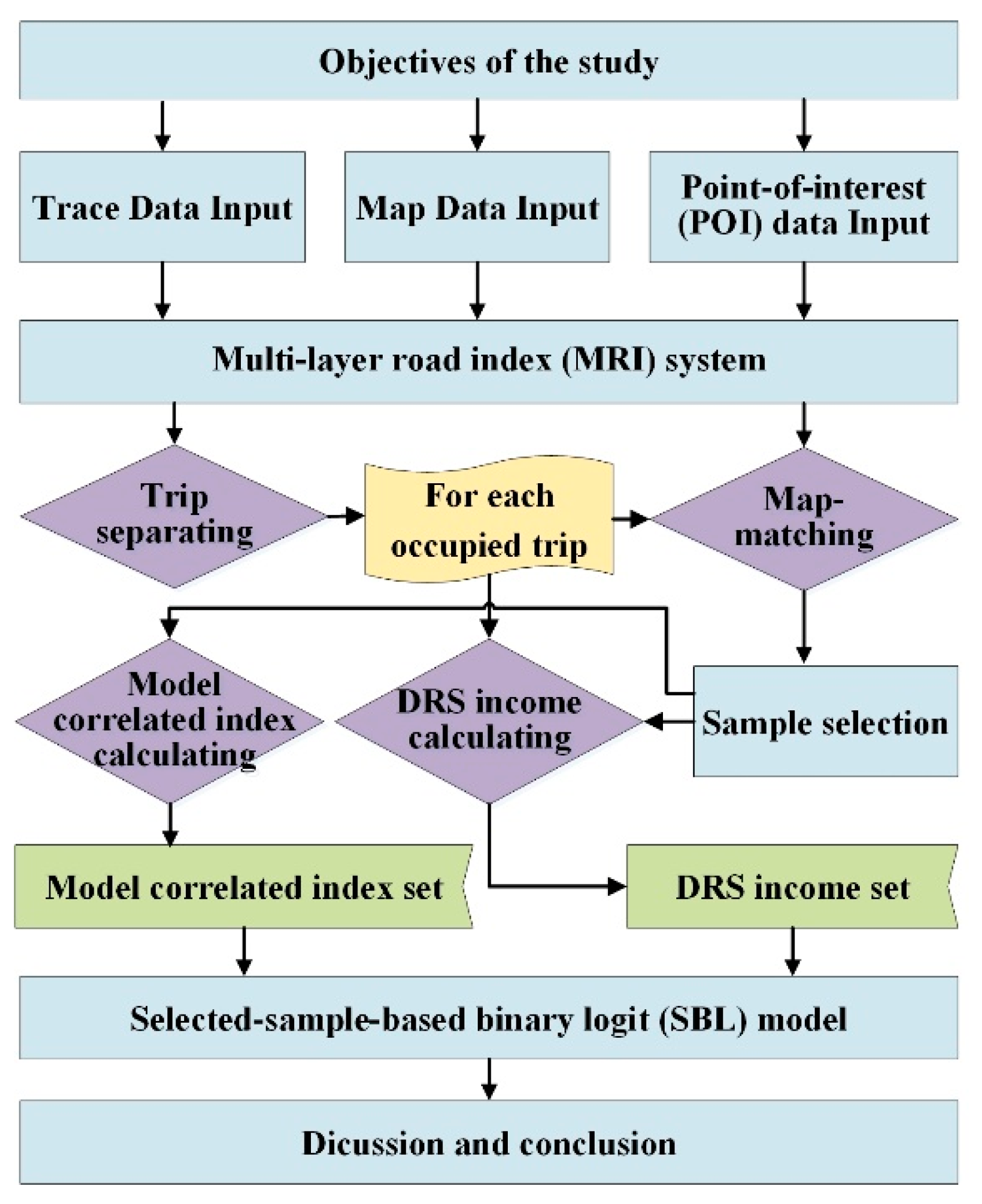
3. Materials and Methods

The Materials and Methods section includes data collection and data extraction processes, the method of income calculation, the definition of indicators affecting income, and the analysis method for causes of income. An overview of the step-by-step study methodology is illustrated in Figure 1.

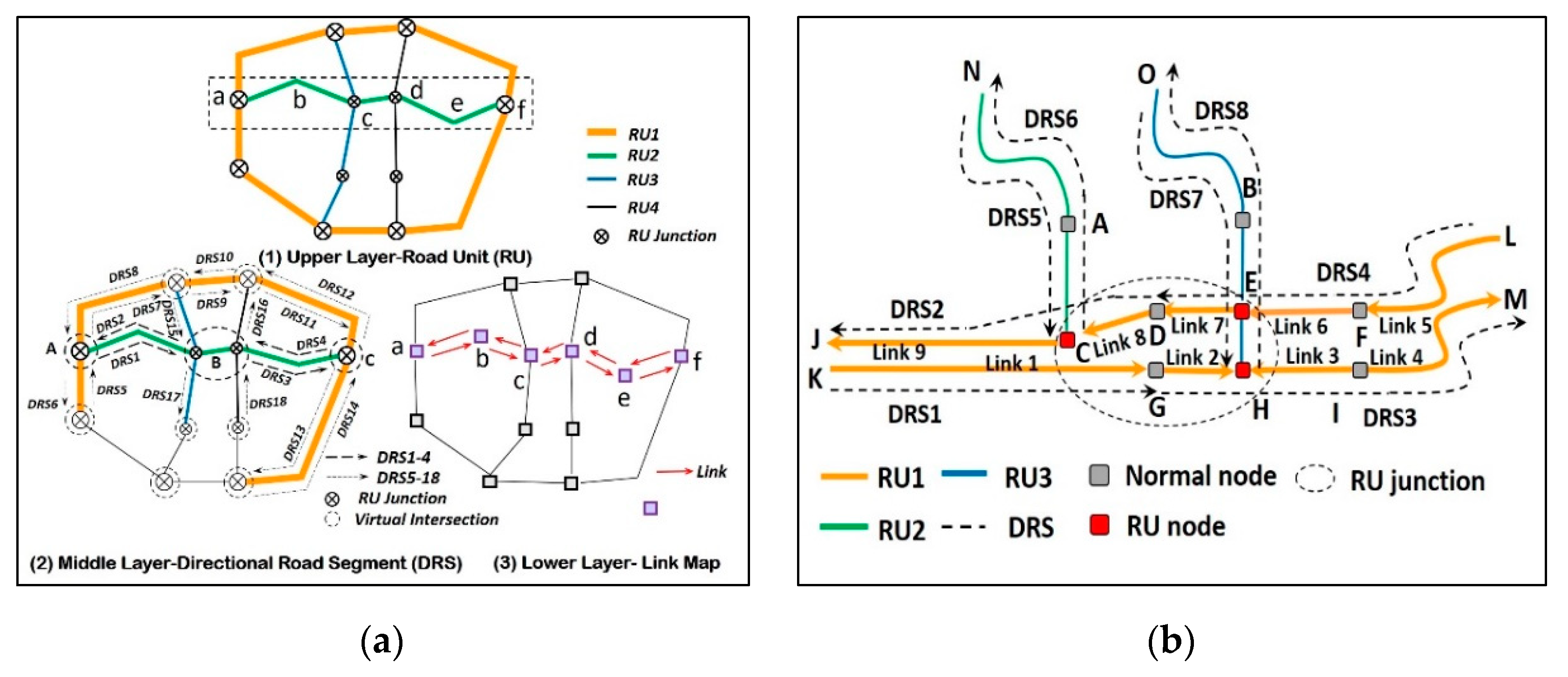
3.1. Multi-Layer Road Index (MRI) System

Most of the current map-matching approaches use algorithms repeatedly, and passively collect and handle local geographic and topological information for each track point; and urban road networks such as multi-layer roads can be particularly complex [39]. Instead of dividing the whole research area into regular grids or suitable TAZs where different types of road segments will be inevitably mixed up, we suggest building a MRI system [40] by extending a road indexing method called “intersection continuity negotiation”, proposed by [41,42].
The MRI system is a technique of pre-processing GIS road networks. It classifies all links in the GIS map of road networks into different groups. Each link belongs to only one group. The links in one group are connected and combined into a road unit that is much longer than any link in the group. A GIS map of road networks pre-processed using the MRI system is called an MRI map, which can help researchers to unveil the features of road networks more deeply, because it supports the analysis at DRS levels.
Given an original topological map of urban road networks G (N, L), where N is the set of road network nodes, and L is the set of the road network links. One or more links constitutes a road segment that connects two adjacent intersections, with attributes such as road name, road direction, and road function classification.
Figure 2a shows the basic component of MRI: a link map layer (the lower layer), a directional road segment layer (the middle layer), and an undirected road unit layer (the upper layer). An MRI system is generated by connecting the three layers, with an illustrative example shown in Figure 2b. The link map layer is derived from the original GIS map. Links, road units (RU), and directional road segments (DRSs) are three different analysis units in the MRI system.
Definition 1 (RU: Road Unit).
For a map G (N, L), a RU represents an undirected virtual traffic corridor that is formed using a series of sequentially connected links. The method in constructing the RU set can be referred to in previous studies.
Definition 2 (DRS: Directional Road Segment).
In the RU networks of map G, the RU junction is denoted as the intersection of two different RUs. For any two adjacent RU junctions, if their distance is no more than a specific value (e.g., 200 m), they are considered as a “virtual intersection”, called the virtual RU junction. The virtual RU junctions and the original RU junctions form the new RU junctions set. Each RU is divided by some of the new RU junctions in the set into a sequence of directional road segment units called DRSs. The DRSs of the same road in the MRI map are paired; each paired DRS represents different directional road segments of the same road.
The MRI system implements the Cross, Continuity and Condition (3C) rules in merging the original map links into DRSs, which makes the system more conducive to revealing the regularity and continuity of the road network, as well as obtaining the driving direction of the taxi driver. Therefore, this proposed MRI system can be extended successfully to the map-matching algorithm, and it is expected to become an invaluable basis for systematic research at the DRS level in the future.

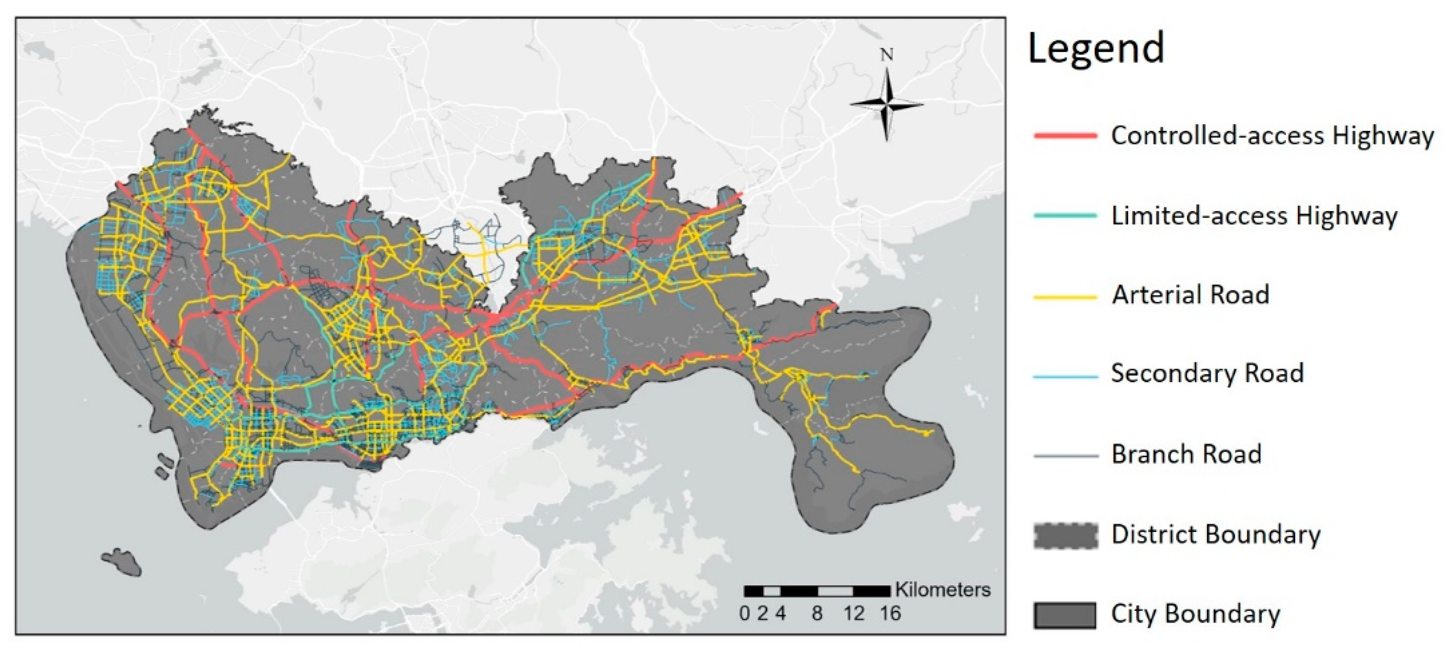
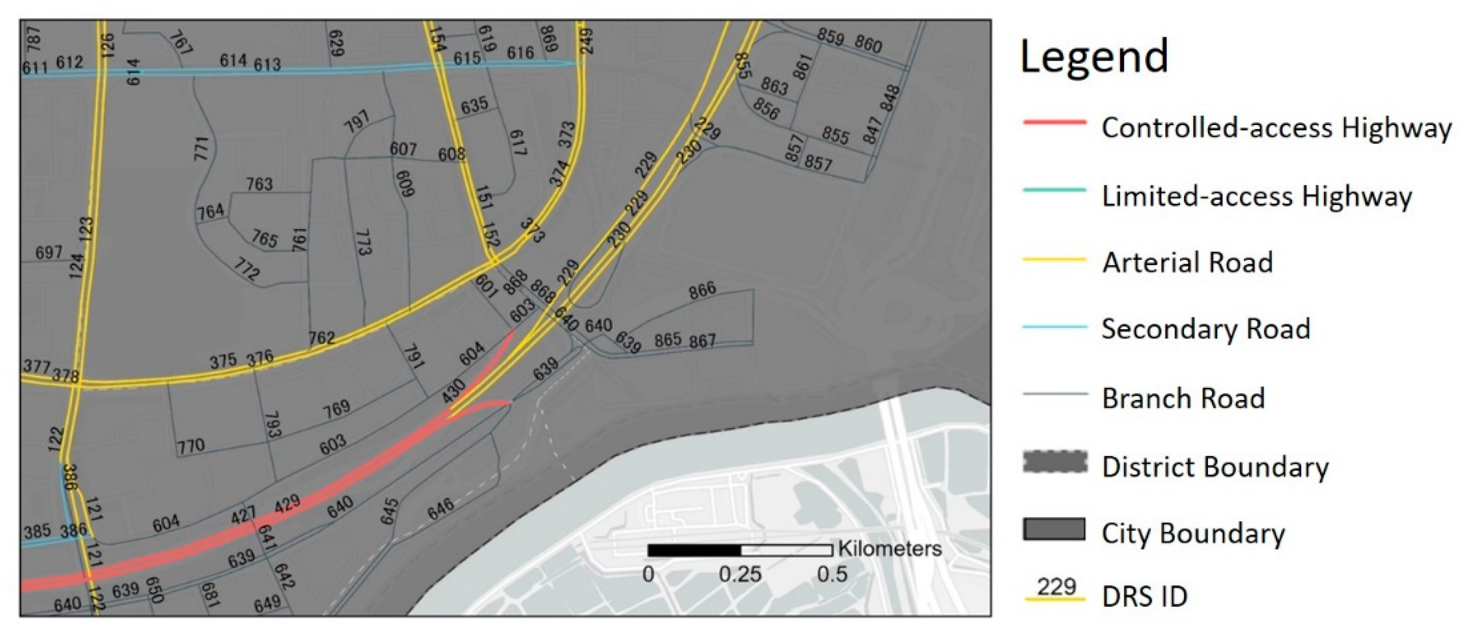
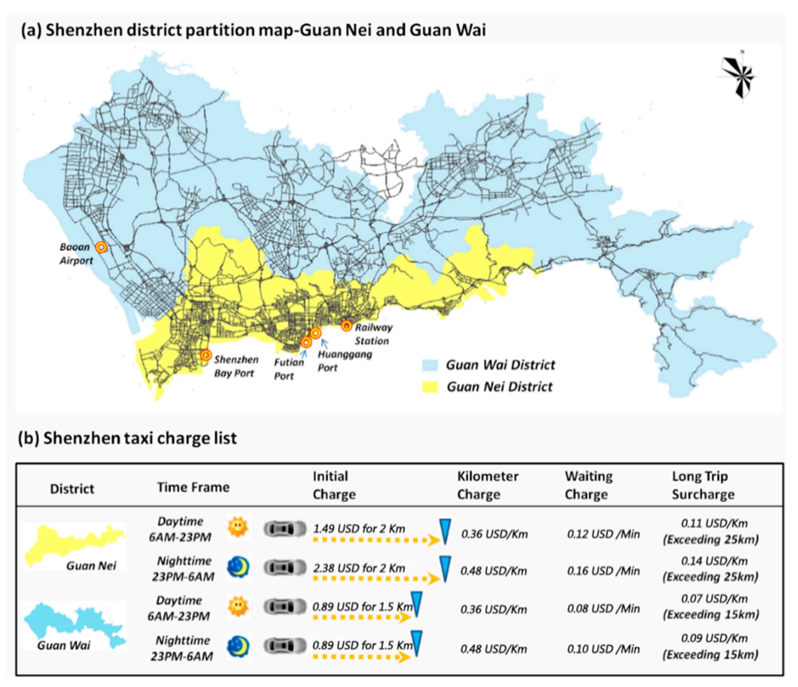
3.2. Study Area and Data

This study selects the main urban area of Shenzhen, China as the case study area. Shenzhen is located at the center of the Pearl River Delta in the south of China, with a land area of 1996.8 km2 and an urban population of over 17 million in 2021. It has six districts, including Luohu, Nanshan, Futian, Baoan, Longgang, and Yantian. It is the first Special Economic Zone (SEZ) city after the institution of reform and the Open-Door Policy in China, in 1979. In the past 30 years, the operation of a market economy has made Shenzhen’s economy develop rapidly, bringing with it a dramatic population increase and spatial expansion. Shenzhen has experienced rapid urbanization at a rate of more than 78% [33]. Its gross domestic product (GDP) increased from RMB 0.2 billion in 1979 to RMB 3066.48 billion in 2021. Shenzhen Metro is the seventh largest system in China, and embraces additional investments. In addition, Shenzhen has established trans-it-supportive policies to promote urban development along transit corridors and to facilitate TOD (transit-oriented development) around transit stations [43]. However, taking Luohu District for example, the coverage of rail stations within 500 m was only 48.6% in the built-up area before 2021 [44]. The mismatch between the demand and supply of rail services is obvious. The traffic condition in Shenzhen has not been improved since the rapid development of rail transit. The worsening of traffic congestion shows that public transportation is still not attractive, or it is maybe losing its appeal. Therefore, research into enhancing cab services as a link between buses and subways is still worthwhile.
The map used in this research is based on the road network of Shenzhen Transportation Planning, which is fitted with an MRI grid consisting of 2476 road units (RU) and 7862 directional road segments (DRSs) derived from 21,115 map links. Figure 3 is the topological road network of the study area, and describes a general view of the different classifications of the roads. The DRSs of the MRI map of Shenzhen were generated based on the layout of the road network. Each DRS is labeled as a number, as described in Figure 4. The basic statistics of the MRI structure of Shenzhen are shown in Table 1.

3.3. Taxi Trace Data

The taxi GPS trajectory data were collected every 30 s during a week from the City of Shenzhen Taxi (COST) database, between 15 January 2015 and 21 January 2015, containing a total of consecutive 194 million passenger track points produced by 15,726 taxis. In order to facilitate the analysis, the trajectory data were recognized as 4.85 million passenger travel paths [45], and each pathway contained a set of continuous tracing points, while the latitude, longitude, and timestamps were associated.

3.4. Point-of-Interest (POI) Data

Points of interest (POIs) provides rich semantics with the mixture of human movement [46], and have been commonly used in various location-based services tools, such as Uber, DiDi, etc. Concerning the taxi market demand, the distribution of POIs in the DRS represent the features of transportation, such as travel purpose, potential travel distance, time consumption, and even travel mode. This research models the features of the taxi income, using the 248,162 POI data points of seven categories in Shenzhen, including the realty/company (3.66%), store (27.28%), transportation (0.04%), hotel (1.93%), entertainment (21.47%), hospital and clinic (0.04%), and parking (0.83%). All of the POIs will be aggregated in the view of the DRSs, and discretized as the model input factors.

3.5. Calculation of Income

According to the taxi charging standards, we counted the payment of each route on the DRSs, based on the MRI system and taxi trace data. The charging standards were classified by the Guan Nei (Nanshan District, Luohu District, Futian District) and Guan Wai (Longgang District, Longhua District, Baoan District) districts, as shown in Figure 5a. The specifics of the charging standards are seen in Figure 5b. Each DRS’s total revenue was calculated by the sum of the route revenue with starting point on this segment.

3.6. Defining Correlated Variables on Each DRS

Based on the established MRI system, four categories of DRS-influencing factors are included, including the road network structure, road section dynamic information, POI distribution, and taxi market operation indicators. These categories are explained as follows.

3.6.1. DRS-Correlated Variables

As a promising application system for map coding, MRI not only provides a complete set of map statistics at the DRS scale, but also makes it possible to analyze the structural characteristics of the road network in depth.

DRS Attributes

For a map G, each map link has a unique DRS label, which in turn is subordinated to a unique RU in representing a continuous traffic corridor. Clearly, the larger the range of the RU to which the DRS belongs (namely, having a larger degree), the more freedom of the path that a trip may choose. Therefore, we use the degree value of the RU as an influencing factor in defining the DRS to which it belongs.
Definition 3 (DRS degree).
DRS degree: For a given RUx of a map G, the DRS degree value is the total number of other RUs directly connected to it, corresponding to the DRS degree of that RU. For a single DRS, it may also be directly connected to other DRSs, so that the upstream and downstream DRSs can be defined.
Definition 4 (Number of upstream/downstream DRSs).
For a given RUx of a map G, the DRS degree value is the total number of other RUs directly connected to it, corresponding to the DRS degree of that RU. For a single DRS, it may also be directly connected to other DRSs, so that the upstream and downstream DRSs can be defined.
Definition 5 (DRS grade).
DRSy describes the yth route of the DRS. For a given DRSy in a map G, a grade value has been applied to indicate the road class, e.g., 1—highway, 2—arterial, 3—secondary, and 4—branch road. The lower the rank value, the higher its road condition and design speed.
Definition 6 (DRS length).
For a given pair of virtual intersections for each DRS, the length is calculated as the Euclidean distance from the center of one end to the other. As shown in Figure 2, the lengths of DRS1 and DRS2 are the Euclidean distances from the virtual intersection A to B.

DRS Dynamics

This type of DRS feature indicates the market dynamics of the DRS. To be more specific, as we mentioned before, the roads become more congested during peak hours, which reduces the market revenue. However, when the congestion dissipates, the revenue increases. Therefore, we use the average speed of the road segment to reflect the actual state of traffic, as no matter what the conditions are, the congestion will affect the traffic volume on the road networks.
Definition 7 (DRS average travel speed).
For a special time period, assuming that Q vehicles passes through the DRSy without intentionally suspending movement (for example, waiting for a passenger), the average travel speed of the DRSy is measured as follows:
a v g S p d y = q = 1 Q d q y q = 1 Q t q y
where, d q y is the total distance of the car q driving on DRSy within the t q y travel time period. According to the four time periods, e.g., the morning peak, evening peak, daytime, and nighttime, the average travel speed of each DRS is generated respectively, using all of the valid occupied taxi trace data.
The average traffic speed of DRS represents the level of road infrastructure supply that adapts to the variety of traffic activities. Considering the taxi demand, it is also important to reveal the dynamic travel characteristics of passengers on each DRS. We notice that, the travel distance not only reflects these characteristics, but also has a direct impact on the service revenue of each trip. Therefore, the proportion of long-distance trips is included in the analysis as follows.
Definition 8 (Long-distance trip ratio of DRS).
For a special time period, a total of P valid trips are supposed staring from DRSy, and the ratio of the long-distance trip DRSy is:
L o n g D i s t y = p = 1 P M A X ( d i s t p y γ | d i s t p y γ | , 0 ) / P  
where d i s t p y represents the travel distance of the trip p, where the starting point is on DRSy. γ is the assumed borderline between short distances and long distances, where the value is taken as 10 km.

Aggregating the POI Data

The distribution of different types of POIs near pick-up points may also reveal some potential taxi demand characteristics, such as possible travel purposes [47,48], the expected travel time or distance [49] and even the mobility pattern [46]. The POIs within 250 m of each DRS were statistically calculated, in order to describe the distribution of POIs by each DRS precisely. It is assumed that the more specific the distribution of POIs spread on the DRSs, the more possible travel demands associated with the POIs.

3.6.2. The Index of DRS Taxi Operation Strategies

In addition to obtaining the attributes of DRSs, the indictors of operation strategies are also obtained, in representing the rules of a taxi picking up passengers and passing through the DRS. This indictor suggests the differences of the service conditions of each DRS.
In the age of ride-hailing, the right operating strategies will boost the earnings of taxi drivers [50]. The literature on the operation strategy has covered passenger searching, passenger delivering, and service area selection [27]. The objectives of the passenger-searching strategy include maximizing profit and maximizing demand coverage [51]. In terms of passenger-delivery strategies and service region preference, choosing similar spatiotemporal areas and dropping off customers as quickly as possible can also increase the profit. Additionally, there are operating strategies with descriptive indicators such as occupied distance, occupied time, capacity utilization [14], etc. In the paper, we defined a new concept, “driver operation strategy”, from the spatial-temporal perspective.
Definition 9 (Ratio of search distance).
This indictor refers to the ratio of deadhead cruising distance to the total cruising distance (deadhead or occupied) generated on DRSy in a certain time period:
R S D y = d i s t e y / d i s t e y + d i s t o y
where, d i s t e y indicates the total deadhead cruising distance on DRSy, and d i s t o y indicates total occupied distance on DRSy.
The higher the RSD, the more likely taxis would move through the road section without passengers; however, this does not always imply a lower travel demand.
Definition 10 (ratio of noninitial price trips).
This indicator is the ratio of the trips that exceed the starting distance on DRSy during a certain period of time:
R N P T y = t r i p e y / t r i p o y
where t r i p e y is the number of the daily trips, except for the trips within the distance of the staring price on DRSy. t r i p o y is the number of occupied trips on DRSy.
Definition 11 (Ratio of long service distance).
For a special time period, this refers to the ratio of the count of occupied passes longer than 10 km on DRSy, to the total count of occupied passes on that segment. A 10 km distance is also taken as the threshold of the long service distance.
R L S D y = d i s t f y / 8000 t r i p e y  
where d i s t f y denotes the total follow distance of picked-up customers on DRSy, which is the part that takes away the initial distance (the initial distance value is 2 km in Guan Nei district). For a long service distance of 10 km, the follow distance is 8 km.
Definition 12 (Ratio of occupied trips).
This indicator represents the ratio of the occupied trips to the overall trips passing through the DRS in a certain period of time.
R O T y = t r i p o y / t r i p y y  
where t r i p y is the total trips that pass through the DRSy.
The correlated variables are described and discretized in Table 2 for the model fitting in the following section.

3.7. Applying the Selected Sample-Based Binary Logit (SBL) Model

The binary logit (BL) model [52] has strong interpretative power for mathematical analysis and the odds ratio. This model is one of the most widely used methods in dealing with multi-scene analysis, from a practical statistical point of view. In general, the dependent variable can be viewed as a dichotomous variable to reflect the positive and negative aspects of a phenomenon. We divide the incomes of all directional road segments into two categories with sample selection. Since the sample size is large enough, the top and bottom 20 percent of DRSs (the sample size is 1865) can be selected to exclude abnormal samples.
Model evaluation: p < 0.05 shows the significance threshold of the explanatory variable. In addition, we used the −2 Log likelihood and Pearson’s Chi-squared statistics to measure the goodness of fit of the model. Then, pseudo-R2 was used to evaluate the proportion of variance explained by the model to the total variance. Finally, the effectiveness and forecast accuracy of the DRS income model was analyzed from the statistical and logical judgment aspects.

4. Experimental Results and Discussion

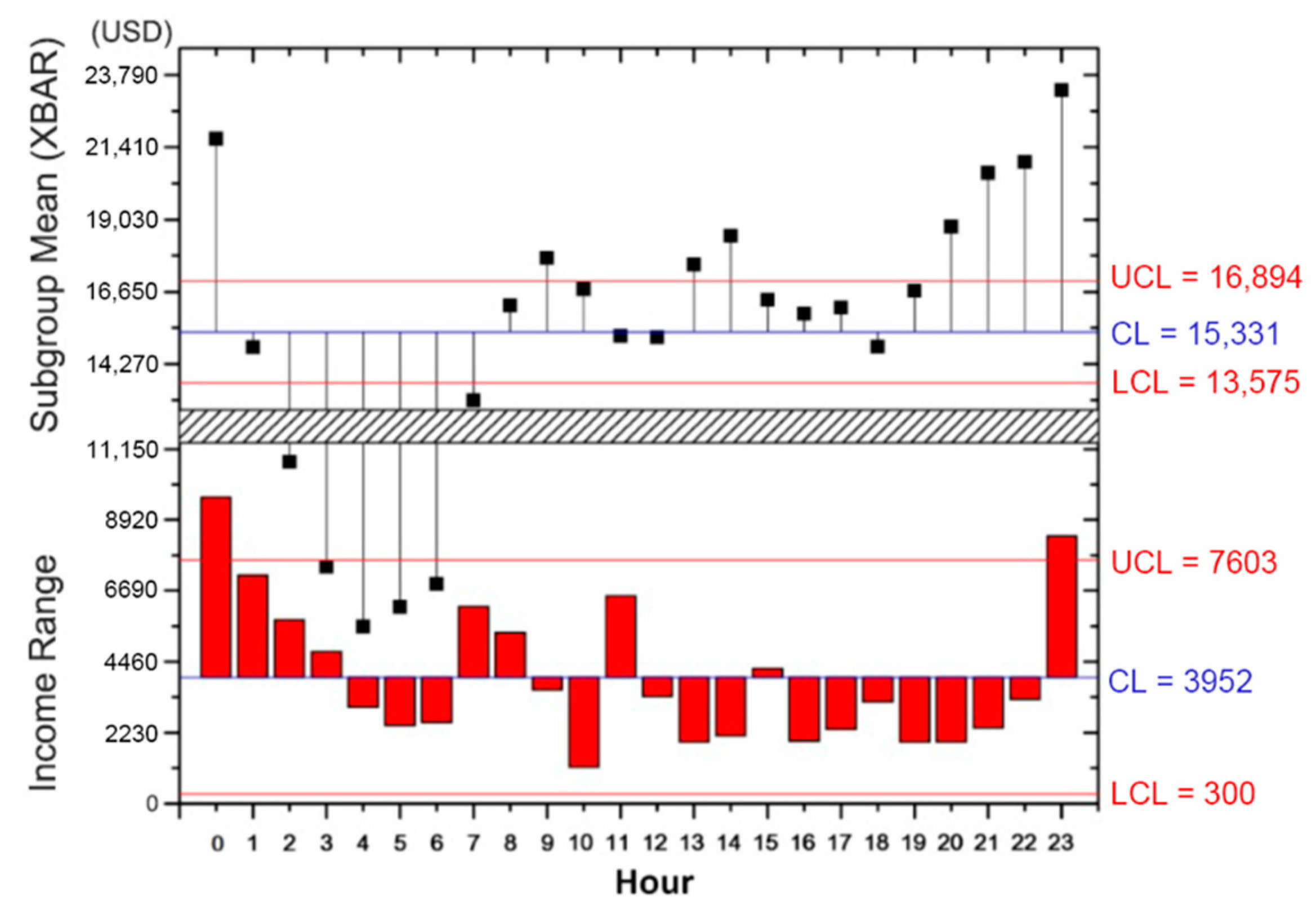
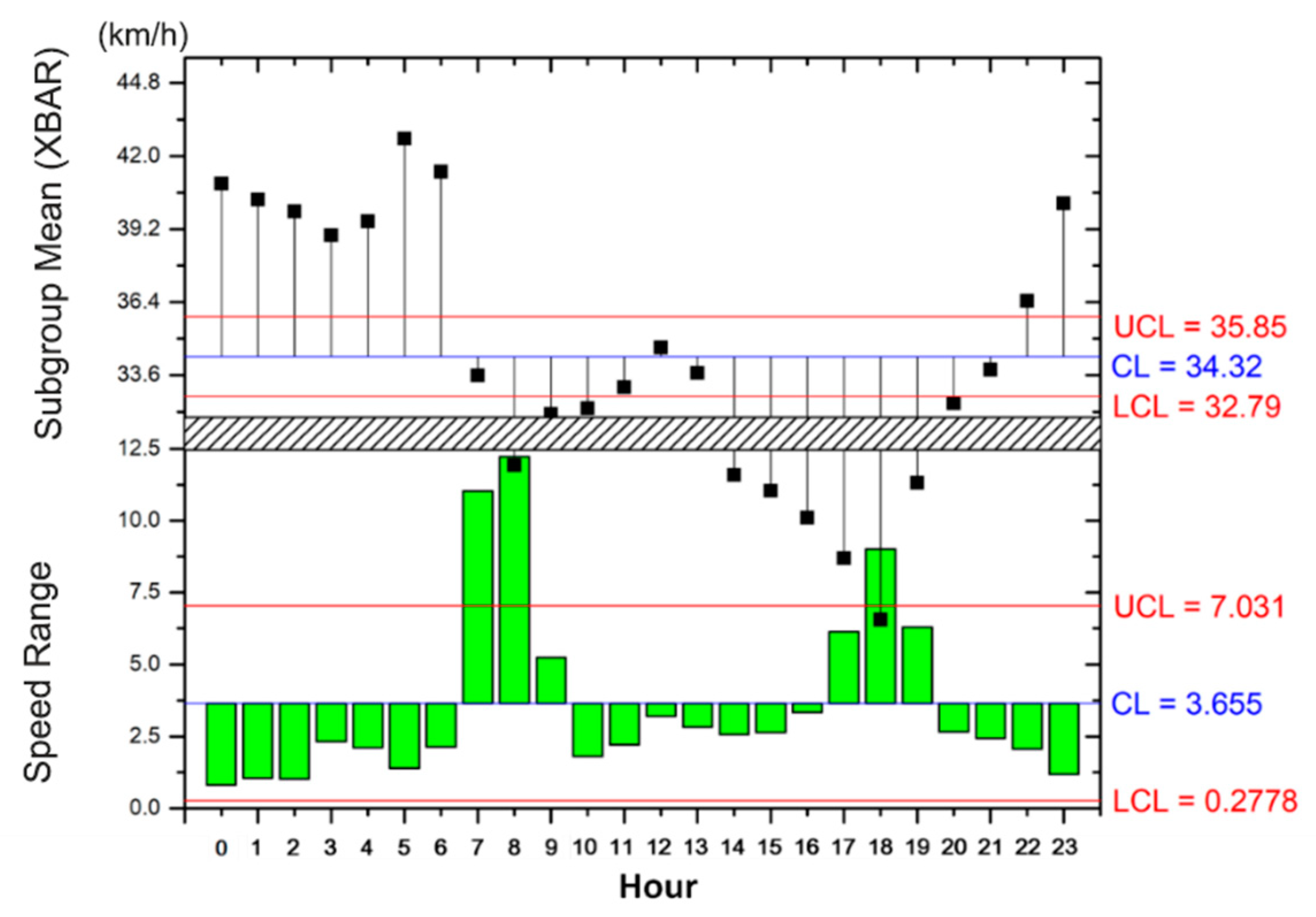
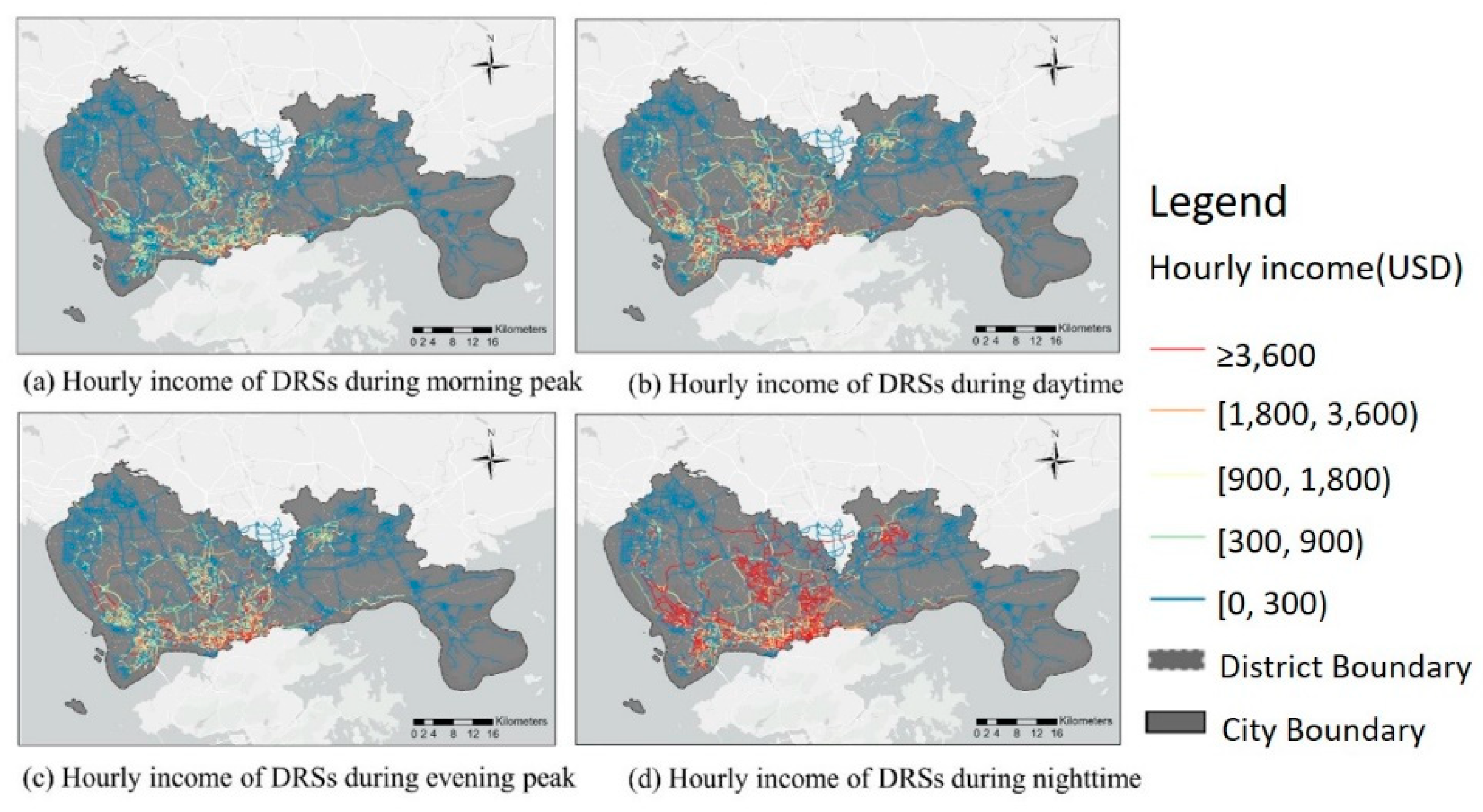
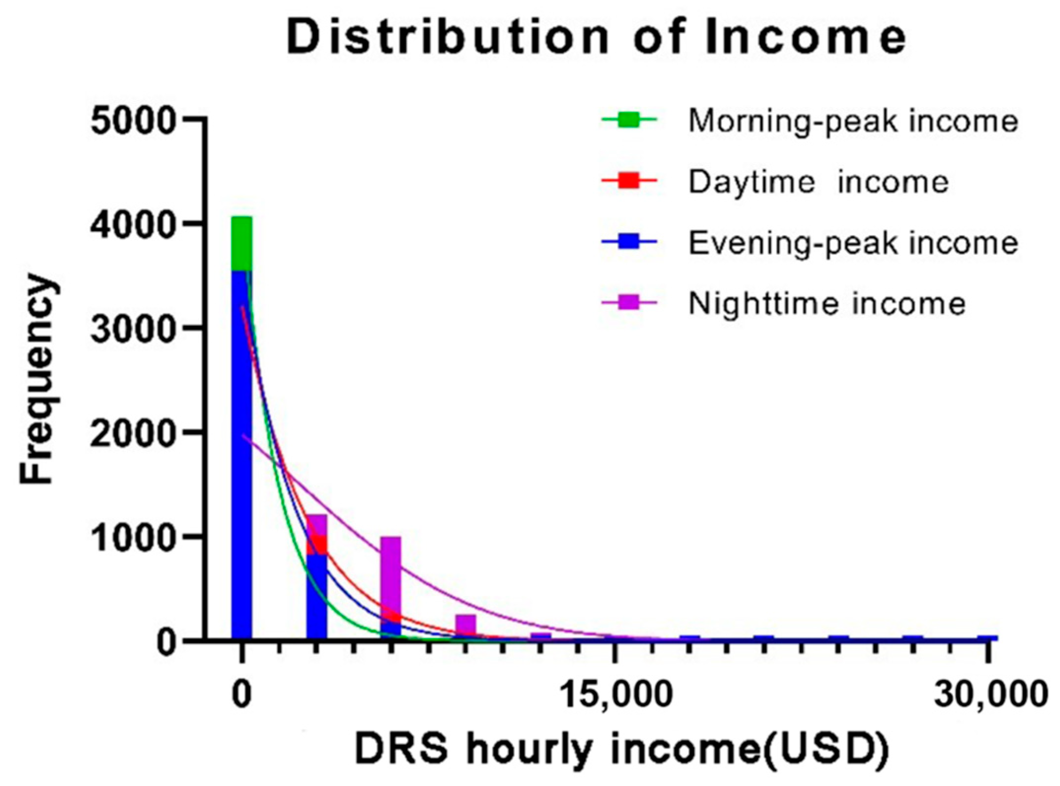
4.1. Distribution of Taxi Income on Directional Road Segments (DRSs)

The total incomes of the DRSs where the taxi journey starts were aggregated. In this research, the sample size was 4661 among the 7862 full-scaled road networks in Shenzhen, where the DRS of the daily travel time was less than 5, namely, a weekly travel time of less than 35, this was excluded. The upper part of Figure 6 illustrates the fluctuation of the income within 24 h, and the lower part shows the hourly income range. To be more specific, the median hourly income for a week is USD 15331 (United States dollars), while the total income is at its lowest level at 4 a.m., suggesting the lowest travel demand at this time. For the morning hours, there is a significant increase in market income, starting at 7 a.m., and with a peak at 9 a.m., which may be largely related to the increase in commuter traffic by taxi in the morning peak. In the evening, the income pinnacle appears at 11 pm. The potential explanation would be the lack of public transportation at that time, because Shenzhen has a large number of leisure events at the end of the day, while the majority of public transportation has been closed.
Figure 7 indicates the regularity of the average speed varying with time at different DRS levels. As can be seen, the average speed exhibits phase characteristics of bimodal variation within the speed restriction of the China’s road traffic safety regulations. It is obvious that there are intensive trip demands during the morning and evening peaks, leading to a significant drop in average speeds. At night, the traffic speed starts to increase, which improves the incomes of taxi drivers with a faster speed and efficient operations. We further divided the data by following four time periods, morning peak (7:00–10:00), daytime (10:00–17:00), evening peak (17:00–22:00), and nighttime (22:00–7:00). Additionally, the income frequency of each time period is calculated. Meanwhile, the spatial distribution of income was more divergent over the whole urban area, as Figure 8 shows, in different periods.
Figure 9 is the distribution histogram of DRS income by time period. This plot indicates that the frequency of the DRS daily income follows an exponential distribution, with a small number of DRSs of high income, and certain DRSs of extremely high income. This shows a good exponential distribution of income for the rest of the time period, except for nighttime, when there is less variation within the DRSs for medium income.

4.2. Result of the SBL Models and Significant Factors

A selected sample-based binary logit (SBL) was used to evaluate the percentage contributions of DRS incomes during the four time periods and all-day. The top and bottom 20/100 rankings of the DRS incomes were selected in representing the income levels, with 1 = high and 0 = low.
Collinearity can be explained as the excessive correlation between independent variables. As the most commonly used methods for the collinearity diagnostics, variance inflation factors (VIF) are estimated before the model fitting. In general, VIF will be not less than 1, and a bigger VIF means that the explanatory variables have a larger collinearity; while the VIF exceeds 4, the variables need to be re-selected or disregarded. Table 3 shows the results of the VIFs, with a majority value of between 1.1 and 3.4. Obviously, there is multicollinearity in the result of the SBL model of all-day, respecting the daytime and evening peak average speeds. With the variables for POIs of Entertainments multicollinearity being serious in all of these five models, this may be closely related to the POI of Store, in representing the consumption characters. Therefore, the POIL. Entertainments was excluded from the input factors for the SBL model fitting, while in the model for all-day, the variables of daytime and evening peak were disregarded.
Table 4 shows the performances of the five SBL models. For each model, the p value is less than 0.05, which means that at least one input factor has been detected for having a significant odds ratio. In addition, the pseudo-R-squared value indicates that the variation degree of dependent variable can be explained by the input factors. Most of the values of pseudo-R2 are over 0.6, representing a good explanatory power of the SBL models and selected variables. Additionally, the accuracy of each model for DRS income is around 85 percent, with a narrow fluctuation of less than 3 percent, except for the accuracy of the nighttime model, which is 70.5%. The nighttime DRS income may be slightly weaker in prediction and explanation, because the sample size is not balanced enough, and the working hours of taxi drivers are characterized by fluctuation.
Table 5 shows the SBL model‘s results of different time periods. The insignificant factors (p > 0.05) have been excluded. Explanations of each variable are shown in Table 2. It is obviously that the DRS attributes (i.e., DegreeL, Grade, Length, DownstreamNumL, AvgSpdL, LongDistL, and POIL) and the taxi operation strategies (i.e., RSDL, RLSDL, ROTL, and RNPTL, respectively) are relevant to the incomes. Specifically, Grade, DownstreamNumL, AvgSpdL, RSDL, RLSDL, and ROTL are the common impact factors correlating with DRS incomes. In general, concerning the taxi operation strategies, RSDL, representing the efficiency of customer search, as well as RLSDL, representing the long-distance ratio of delivery passengers, had highly negative impacts on the incomes, representing the ROTL of the passenger turnover ratio boost incomes. In the all-day model, the indictor of ODDs indicates that drivers should certainly be more hard working or flexible, and cruise to increase their incomes (positive odd ratio (OR) of ROTL = 3.730; negative OR of RLSDL = 0.323; negative OR of RSDL = 0.087).
The degree of the DRS dominates the attractiveness of the road segment, while the grade of the DRS determines its accessibility. The number of the downstream DRS increases the probability that passengers choose the current DRS as the starting point, and the average travel speed also reflects the efficiency of the taxi transport. For example, in the all-day model, positive OR of DownstreamNumL = 2.612, positive OR of DegreeL = 1.833, negative OR of Grade = 0.611, and negative OR of AvgSpdL = 0.570. This shows that the importance of the road in the road network, the connection form, and the degree of accessibility will all have an impact on the DRS income.
It is worth noting though that POI is also an important factor impacting on incomes, but with different specific types in each model. Specifically, five types of POI appeared to be the significant factors distributed throughout various periods, including “Hotel” (only nighttime), “Scenic” (all periods except nighttime), “Realty&Company” (all periods except nighttime), “transportation” (only nighttime), and “Hospital&Clinic” (all periods except daytime).
General analysis: Grade, AvgSpdL, RSD, and RLSD are negatively correlated with the DRS income. The lower Grade indicates the lower level of activities, which leads lower taxi market demands and incomes. Nevertheless, the lower AvgSpdL is related to a higher building density and taxi market demand, which refers to a higher income. Interestingly, a higher RLSD does not lead to an increase in DRS income, but rather, to a decrease. This result suggests that distant travel will decrease the incomes because of its time consuming nature. The number of downstream DRS, Degree, and the ROT are positively correlated with the incomes. This result indicates that more downstream DRSs, a greater degree, and a higher incidence of carrying passengers, with more potential taxi demands directly causes a higher revenue concentration effect in the market.
The only difference is that RNPT is positively correlated with the all-day (coefficient 0.537, p < 0.05) and daytime models (coefficient 0.451, p < 0.05), and negatively correlated with the nighttime model (coefficient −0.364, p < 0.05). This finding implies that income is reduced as a result of more long-distance trips taken at night.

4.3. Discussion and Implications

Although the OLS model has indicated the main factors determining DRS income, the significance of each indicator varies over time. More specifically, the differences between the results of these five models are as follows:
(1)
The DRS length only impacts on the nighttime income. This result may be attributed to the sparse taxi demands, where the longer the length of the DRS, the higher the incomes.
(2)
Degree and LongDist have no impact on the nighttime model, which are due to the high driving speed and the dispersions of the travel destination at nighttime.
(3)
The number of upstream DRSs only has a positive impact on market revenue during the morning peak. This phenomenon can be explained as the greater number of upstream and downstream DRSs, which contribute to alleviating the traffic congestion, as well as increasing the incomes. This result also indicates that the travel demand is more intensive in the morning rush hours compared with other time periods.
(4)
The POIL of Realty/Company, Hospital/Clinic, and Park has a greater contribution to the DRS income in the peak hours and all-day models, comparing to the other POI type. The Hospital/Clinic-type POI is not related to the DRS income in the daytime model, as it is consistent with the travel characteristics of patients. The nighttime model has a distinctive feature, in that the POI of Transportation (OR 1.431; p < 0.05) has a positive impact on DRS incomes, in accordance with the land use of Hotel (OR 1.239; p < 0.05) and Hospital/Clinic (OR 1.419; p < 0.05) at night.
(5)
RNPT only has an impact in the model of peak traffic hours, owing to the traffic congestion causing incomplete trips within the starting distance.
The key contribution of this study is that, instead of using the driver as the statistical unit, the branch road section is utilized to integrate taxi income and to analyze the elements that affect income level. The taxi GPS trajectory is accurately matched by direction, using a new map-matching technique. At the same time, it increases the effect of the characteristics of the branch road itself on income, in addition to taking traditional taxi demand, driver service strategy indicators, and driving speed into account. The behavioral motive indicating driver intelligence was left out of the influencing elements due to the lack of sufficient driver information. The impacts of significant influencing factors on the income levels of DRSs are summarized as follows:
(1)
Taxi operation strategies are important aspects in determining DRS income, among which, the RSD is the most indicative factor in describing the service efficiency. These results are consistent with findings in similar research [35], which indicates that high-income DRSs often have shorter search distances.
(2)
The number of downstream DRSs is the determinant factor affecting incomes. From the angle of a complex network, more travel options coinciding with the taxi driving direction contribute more to the DRS income than the degree of interconnection.
(3)
In the nighttime model, AvgSpdL is the only significant indicator affecting income, and it is also the only controllable factor that can increase the efficiency of the distribution performance.
(4)
In the evening peak model, AvgSpdL is also a key factor in influencing the option of travel path. During the evening peak, this indictor is particular important in avoiding the congested section of the road, to drive up the speed and increase the income. These results are consistent with findings in similar research [37], which found that the income is greatly affected by traffic conditions in the evening peak hours.
(5)
POI types have different effects on DRS income at different time periods, but “Scenic” and “Realty&Company” are constant factors that affect income. As with more “Realty&Company” being more likely to form larger crowds, the surrounding roads with “Scenic” will also generate a lot of taxi demand for foreign tourists, thereby increasing the income. These results are consistent with findings in similar research [38].

5. Conclusions

This research uses the SBL model in investigating the impact factors of the DRS incomes. We have made up for the blankness of analyzing taxi drivers’ incomes from the perspective of DRSs. Four kinds of influencing factors have been classified according to the impacts of different time periods, to improve the accuracy of the analysis of DRS income. The major findings are included as follows:
(1)
There exists a marked difference in DRS incomes. The average hourly incomes within the study hours have a mean of USD 15,331 and a standard deviation of USD 3952. The gap between the lowest average hourly income of DRS and the highest average hourly income of DRS, which approaches USD 17,000, is larger.
(2)
The main factors in income analysis are the factors used to represent taxi operation strategies and the number of downstream DRSs. RSD (coefficient −2.445), RLSD (coefficient −1.13), and ROT (coefficient 1.316) are significant operational measures of the taxi market, according to the SBL all-day model, which was tested over time. The daytime, nighttime, and all-day models are all possible with RNPT. In addition, DownstreamNumL is a very important element of its positive effect in the five models, which were found to have ORs of 2.612, 2.133, 2.971, 2.496, and 1.501 during the all-day, morning peak, daytime, evening peak, and nighttime, respectively. This conclusion can be used as a starting point for further research into the taxi market revenue, from both the driver and DRS perspectives.
(3)
The factors that influence incomes in different time periods are completely different. DRSs with more real estate/companies, hospitals with many upstream roads, degrees, and high road grades are more high-income DRSs during the morning peak. The DRSs with several realty/companies, hospitals, and parks nearby, as well as more downstream roads, more degrees, and higher road ranks, are high-income areas during the evening peak. During the daytime, high-income DRSs congregate in areas with a lot of real estate/companies and parks, as well as a lot of downstream roads, a lot of degrees, and a lot of long-distance travel. DRS income distribution is more scattered at night, with fewer impact factors, but a higher grade, more downstream, longer road length, and adjacent hotels, traffic stations, and hospitals corresponding to high-income road sections were also identified.
These findings quantitatively demonstrate the influence of road attributes on the spatiotemporal distribution of the income, from a novel directional perspective. For different time periods, a summary of the characteristics of the high-income DRSs can provide new ideas for taxi industry managers to balance the income levels of drivers. A selected order delivery process by the managers can reduce the proportion of low-income drivers, as well as improving the overall efficiency of taxi drivers. Two suggestions are being recommended for the taxi industry managers: (1) Taxi charge rules should take traffic circumstances into account, especially in locations where the average speed is excessively slow during the morning and evening peak hours. (2) The vehicle dispatch system should offer a fair opportunity to drivers traveling to high-income areas.
In this research, a feasible model for large-scale DRS data mining operation is provided. As far as we are aware, this is the first demonstration of how to investigate taxi revenue with a procedure of map preprocessing, and the trajectory matching method. For future study, this method could be utilized in analyzing the impact of taxis on urban carbon emissions, finding restricted areas, road sections, and directions for taxi drivers, controlling the total amount of taxis, etc. Although this article only focuses on the physical road elements that drive DRS incomes, the fundamental method and research structure can be utilized for relevant factors, such as human characteristics. In the following phase, we plan to gather private information on drivers, such as their gender, age, and whether or not they have children, etc., and analyze how these factors may affect taxi revenues.

Author Contributions

Conceptualization, Ming Cai; methodology, Shuxin Jin; data curation, Zhouhao Wu; writing—original draft preparation, Shuxin Jin; writing—review and editing, Tong Shen; visualization, writing—review, Di Wang. All authors have read and agreed to the published version of the manuscript.

Funding

This research was funded by the Fundamental Research Funds for the Central Universities, Sun Yat-sen University (Grant number 22dfx08), the National Key R&D Program of China (Grant number 2020YFB1600400), the Special Scientific Research Program of the Education Department of Shaanxi Province of China (Grant number 19JK0382).

Data Availability Statement

The data presented in this study are available on request to the corresponding author.

Conflicts of Interest

The authors declare no conflict of interest.

References

  1. Lozano, J.A.; Macías, J.A.G.; Chávez, E. Crowd location forecasting at points of interest. Int. J. Ad Hoc Ubiquitous Comput. 2015, 18, 191–204. [Google Scholar] [CrossRef]
  2. Ashkrof, P.; Correia, G.H.D.A.; Cats, O.; van Arem, B. Understanding ride-sourcing drivers’ behaviour and preferences: Insights from focus groups analysis. Res. Transp. Bus. Manag. 2020, 37, 100516. [Google Scholar] [CrossRef]
  3. Castro, P.S.; Zhang, D.; Chen, C.; Li, S.; Pan, G. From taxi GPS traces to social and community dynamics. ACM Comput. Surv. 2013, 46, 1–34. [Google Scholar] [CrossRef]
  4. Chen, Y.; Fu, Q.; Zhu, J. Finding next high-quality passenger based on spatio-temporal big data. In Proceedings of the 2020 IEEE 5th International Conference on Cloud Computing and Big Data Analytics (ICCCBDA), Chengdu, China, 10–13 April 2020; pp. 447–452. [Google Scholar]
  5. Cramer, J.; Krueger, A.B. Disruptive Change in the Taxi Business: The Case of Uber. Am. Econ. Rev. 2016, 106, 177–182. [Google Scholar] [CrossRef] [Green Version]
  6. Duong, H.L.; Chu, J.; Yao, D. Taxi Drivers’ Response to Cancellations and No-Shows: New Evidence for Reference-Dependent Preferences. Manag. Sci. 2022. [Google Scholar] [CrossRef]
  7. Gao, Y.; Xu, P.; Lu, L.; Liu, H.; Liu, S.; Qu, H. Visualization of Taxi Drivers’ Income and Mobility Intelligence. In International Symposium on Visual Computing; Springer: Berlin/Heidelberg, Germany, 2012; pp. 275–284. [Google Scholar] [CrossRef]
  8. He, Z.; Xi-Wei, S.; Zhuang, L.; Nie, P. On-line map-matching framework for floating car data with low sampling rate in urban road networks. IET Intell. Transp. Syst. 2013, 7, 404–414. [Google Scholar] [CrossRef]
  9. Hu, B.; Xia, X.; Sun, H.; Dong, X. Understanding the imbalance of the taxi market: From the high-quality customer’s perspective. Phys. A Stat. Mech. Its Appl. 2019, 535. [Google Scholar] [CrossRef]
  10. Liu, X.; Sun, L.; Sun, Q.; Gao, G. Spatial Variation of Taxi Demand Using GPS Trajectories and POI Data. J. Adv. Transp. 2020, 2020, 7621576. [Google Scholar] [CrossRef]
  11. Lai, X.; Fu, H.; Li, J.; Sha, Z. Understanding drivers’ route choice behaviours in the urban network with machine learning models. IET Intell. Transp. Syst. 2018, 13, 427–434. [Google Scholar] [CrossRef]
  12. Liu, L.; Andris, C.; Ratti, C. Uncovering cabdrivers’ behavior patterns from their digital traces. Comput. Environ. Urban Syst. 2010, 34, 541–548. [Google Scholar] [CrossRef]
  13. Liu, Q.; Ding, C.; Chen, P. A panel analysis of the effect of the urban environment on the spatiotemporal pattern of taxi demand. Travel Behav. Soc. 2019, 18, 29–36. [Google Scholar] [CrossRef]
  14. Lv, Q.; Qiao, Y.; Ansari, N.; Liu, J.; Yang, J. Big Data Driven Hidden Markov Model Based Individual Mobility Prediction at Points of Interest. IEEE Trans. Veh. Technol. 2016, 66, 5204–5216. [Google Scholar] [CrossRef]
  15. Maruthasalam, A.P.; Roy, D.; Venkateshan, P. Refuse or Accept?: Analysis of Taxi Driver Operating Strategies in E-Hailing Platforms. Soc. Sci. Electron. Publ. 2018. [Google Scholar] [CrossRef]
  16. Menard, S.W. Quantitative Applications in the Social Sciences. In Applied Logistic Regression Analysis; Sage Pubns: Thousand Oaks, CA, USA, 2013. [Google Scholar]
  17. Naji, H.; Wu, C.; Hui, Z.; Li, L. Towards understanding the impact of human mobility patterns on taxi drivers’ income based on GPS data: A case study in Wuhan—China. In Proceedings of the 2017 4th International Conference on Transportation Information and Safety (ICTIS), Banff, AB, Canada, 8–10 August 2017; pp. 1152–1160. [Google Scholar] [CrossRef]
  18. Nie, Y. How can the taxi industry survive the tide of ridesourcing? Evidence from Shenzhen, China. Transp. Res. Part C Emerg. Technol. 2017, 79, 242–256. [Google Scholar] [CrossRef]
  19. Oleyaei-Motlagh, S.Y.; Vela, A. Inferring demand from partially observed data to address the mismatch between demand and supply of taxis in the presence of rain. arXiv 2019, arXiv:1903.06619. [Google Scholar]
  20. Ou, G.; Wu, Y.; Wang, G.; Guo, Z. Big-data-based analysis on the relationship between taxi travelling patterns and taxi drivers’ incomes. In Proceedings of the 2019 16th International Conference on Service Systems and Service Management, ICSSSM, Shenzhen, China, 13–15 July 2019; pp. 1–6. [Google Scholar] [CrossRef]
  21. Porta, S.; Crucitti, P.; Latora, V. The network analysis of urban streets: A dual approach. Phys. A Stat. Mech. Its Appl. 2006, 369, 853–866. [Google Scholar] [CrossRef] [Green Version]
  22. Qin, G.; Li, T.; Yu, B.; Wang, Y.; Huang, Z.; Sun, J. Mining factors affecting taxi drivers’ incomes using GPS trajectories. Transp. Res. Part C Emerg. Technol. 2017, 79, 103–118. [Google Scholar] [CrossRef] [Green Version]
  23. Qu, M.; Zhu, H.; Liu, J.; Liu, G.; Xiong, H. A cost-effective recommender system for taxi drivers. In Proceedings of the 20th ACM SIGKDD International Conference on Knowledge Discovery and Data Mining, New York, NY, USA, 24–27 August 2014. [Google Scholar] [CrossRef]
  24. Rong, H.; Zhou, X.; Yang, C.; Shafiq, Z.; Liu, A. The rich and the poor: A Markov decision process approach to optimizing taxi driver revenue efficiency. In Proceedings of the International Conference on Information and Knowledge Management, Beijing, China, 24–28 October 2016; pp. 2329–2334. [Google Scholar] [CrossRef] [Green Version]
  25. Salanova, J.M.; Estrada, M.; Aifadopoulou, G.; Mitsakis, E. A review of the modeling of taxi services. Procedia-Soc. Behav. Sci. 2011, 20, 150–161. [Google Scholar] [CrossRef] [Green Version]
  26. Scellato, S.; Musolesi, M.; Mascolo, C.; Latora, V.; Campbell, A.T. NextPlace: A spatio-temporal prediction framework for pervasive systems. In Proceedings of the International Conference on Pervasive Computing, San Francisco, CA, USA, 12–15 June 2011; pp. 152–169. [Google Scholar] [CrossRef] [Green Version]
  27. Sirisoma, R.M.N.T.; Wong, S.C.; Lam, W.H.K.; Wang, D.; Yang, H.; Zhang, P. Empirical evidence for taxi customer-search model. Proc. Inst. Civ. Eng.-Transp. 2010, 163, 203–210. [Google Scholar] [CrossRef] [Green Version]
  28. Sun, L.; Zhang, D.; Chen, C.; Castro, P.S.; Li, S.; Wang, Z. Real Time anomalous trajectory detection and analysis. Mob. Netw. Appl. 2012, 18, 341–356. [Google Scholar] [CrossRef]
  29. Tang, L.; Sun, F.; Kan, Z.; Ren, C.; Cheng, L. Uncovering distribution patterns of high performance taxis from big trace data. ISPRS Int. J. Geo-Inf. 2017, 6, 134. [Google Scholar] [CrossRef] [Green Version]
  30. Tang, L.; Zheng, W.; Wang, Z.; Hong, X.U.; Hong, J.; Dong, K. Space Time Analysis on the Pick-up and Drop-off of Taxi Passengers Based on GPS Big Data. J. Geo-Inf. Sci. 2015, 17, 1179–1186. [Google Scholar] [CrossRef]
  31. Tu, J.; Duan, Y. Detecting Congestion and Detour of Taxi Trip via GPS Data. In Proceedings of the 2017 IEEE 2nd International Conference on Data Science in Cyberspace, DSC 2017, Shenzhen, China, 26–29 June 2017; pp. 615–618. [Google Scholar] [CrossRef]
  32. Wang, D.; Miwa, T.; Morikawa, T. Interrelationships between traditional taxi services and online ride-hailing: Empirical evidence from Xiamen, China. Sustain. Cities Soc. 2022, 83. [Google Scholar] [CrossRef]
  33. Wang, D.; Miwa, T.; Morikawa, T. Comparative Analysis of Spatial–Temporal Distribution between Traditional Taxi Service and Emerging Ride-Hailing. ISPRS Int. J. Geo-Inf. 2021, 10, 690. [Google Scholar] [CrossRef]
  34. Wang, W.; Pan, L.; Yuan, N.; Zhang, S.; Liu, D. A comparative analysis of intra-city human mobility by taxi. Phys. A Stat. Mech. Its Appl. 2015, 420, 134–147. [Google Scholar] [CrossRef]
  35. Wang, Y.; Wu, Z.; Li, C. The Complexity of Large-scale Urban Networks: A Comparative Study in China. In Proceedings of the Transportation Research Board Annual Meeting, Washington, DC, USA, 11–15 January 2015; pp. 15–4997. [Google Scholar]
  36. Wong, R.; Szeto, W.; Wong, S.C.; Yang, H. Modelling multi-period customer-searching behaviour of taxi drivers. Transp. B Transp. Dyn. 2013, 2, 40–59. [Google Scholar] [CrossRef]
  37. Wu, Z.; Xie, J.; Wang, Y.; Nie, Y.M. Map matching based on multi-layer road index. Transp. Res. Part C Emerg. Technol. 2020, 118, 102651. [Google Scholar] [CrossRef]
  38. Yang, J.; Su, P.; Cao, J. On the importance of Shenzhen metro transit to land development and threshold effect. Transp. Policy 2020, 99, 1–11. [Google Scholar] [CrossRef]
  39. Ye, Y.; Zheng, Y.; Chen, Y.; Feng, J.; Xie, X. Mining Individual Life Pattern Based on Location History. In Proceedings of the 2009 Tenth International Conference on Mobile Data Management: Systems, Services and Middleware, Taipei, Taiwan, 18–20 May 2009; pp. 1–10. [Google Scholar] [CrossRef]
  40. Yuan, C.; Geng, X.; Mao, X. Taxi High-Income Region Recommendation and Spatial Correlation Analysis. IEEE Access 2020, 8, 139529–139545. [Google Scholar] [CrossRef]
  41. Yuan, C.; Wu, D.; Wei, D.; Liu, H. Modeling and Analyzing Taxi Congestion Premium in Congested Cities. J. Adv. Transp. 2017, 2017, 2619810. [Google Scholar] [CrossRef] [Green Version]
  42. Yuan, J.; Zheng, Y.; Zhang, L.; Xie, X.; Sun, G. Where to find my next passenger. In Proceedings of the 13th international Conference on Ubiquitous Computing, Beijing, China, 17–21 September 2011; pp. 109–118. [Google Scholar] [CrossRef]
  43. Yuan, N.J.; Zheng, Y.; Zhang, L.; Xie, X. T-Finder: A Recommender System for Finding Passengers and Vacant Taxis. IEEE Trans. Knowl. Data Eng. 2012, 25, 2390–2403. [Google Scholar] [CrossRef]
  44. To Create a “Main Position” for Social Integration between Shenzhen and Hong Kong, Shenzhen Luohu Strives to Build a Pioneer Area for the Shenzhen-Hong Kong Port Economic Belt. Available online: http://www.tzb.sz.gov.cn/xwzx/gzdt/gqgz/content/post_825145.html (accessed on 16 July 2022).
  45. Yu, X.; Gao, S.; Hu, X.; Park, H. A Markov decision process approach to vacant taxi routing with e-hailing. Transp. Res. Part B Methodol. 2019, 121, 114–134. [Google Scholar] [CrossRef]
  46. Zhang, D.; Sun, L.; Li, B.; Chen, C.; Pan, G.; Li, S.; Wu, Z. Understanding Taxi Service Strategies From Taxi GPS Traces. IEEE Trans. Intell. Transp. Syst. 2014, 16, 123–135. [Google Scholar] [CrossRef]
  47. Zhang, W.; Huang, B.; Luo, D. Effects of land use and transportation on carbon sources and carbon sinks: A case study in Shenzhen, China. Landsc. Urban Plan. 2014, 122, 175–185. [Google Scholar] [CrossRef]
  48. Zheng, Y. Trajectory Data Mining. ACM Trans. Intell. Syst. Technol. 2015, 6, 1–41. [Google Scholar] [CrossRef]
  49. Zheng, Y.; Capra, L.; Wolfson, O.; Yang, H. Urban Computing. ACM Trans. Intell. Syst. Technol. 2014, 5, 1–55. [Google Scholar] [CrossRef]
  50. Zhang, Y.; Zhong, M.; Jiang, Y. A data-driven quantitative assessment model for taxi industry: The scope of business ecosystem’s health. Eur. Transp. Res. Rev. 2017, 9, 23. [Google Scholar] [CrossRef]
  51. Zheng, Z.; Rasouli, S.; Timmermans, H. Modeling taxi driver search behavior under uncertainty. Travel Behav. Soc. 2020, 22, 207–218. [Google Scholar] [CrossRef]
  52. Zhou, B.; Ma, L.; Hu, J.; Wu, S.; He, G. Extraction of Urban Hotspots and Analysis of Spatial interaction Based on Trajectory Data Field: A Case Study of Shenzhen City. Trop. Geogr. 2019, 39, 117–124. [Google Scholar] [CrossRef]
Figure 1. Study methodology flow chart.
Ijgi 11 00431 g001
Figure 2. Multi-layer road index (MRI) system. (a) Three layers in an MRI system. (b) An example of the MRI system.
Ijgi 11 00431 g002
Figure 3. Road network structure of Shenzhen (the source of the geographical background is Mapbox).
Ijgi 11 00431 g003
Figure 4. Example of directional road segments (DRSs) of Shenzhen (the source of the geographical background is Mapbox).
Ijgi 11 00431 g004
Figure 5. Shenzhen district partition and taxi charge list (the source of the geographical background is Mapbox).
Ijgi 11 00431 g005
Figure 6. Trend diagram for income on DRSs.
Ijgi 11 00431 g006
Figure 7. Trend diagram for speed on DRSs.
Ijgi 11 00431 g007
Figure 8. Spatial distributions of incomes (the source of the geographical background is Mapbox).
Ijgi 11 00431 g008
Figure 9. Distribution histogram for DRS income at different time periods.
Ijgi 11 00431 g009
Table 1. Basic statistics of the MRI system of Shenzhen.
Road LevelLinkRUDRSDRS/RU Ratio
AmountLength (km)AmountLength (km)AmountLength (km)
Highway2901.931918.271482.357.79
Arterial road79400.283197.0522860.987.17
Secondary road53540.226431.1519200.392.99
Branch road75310.2414950.7435080.312.35
Total211150.2724761.7378620.593.18
Table 2. DRS-correlated variable description and classified list.
VariableDescriptionValue Type
Level of DRS AttributesDegreeLThe level of road degree of current DRS. If the road degree value of the RU containing current DRS is less than 12, DegreeL = 1; not less than 25, DegreeL = 3; otherwise, DegreeL = 2.Fixed
GradeThe road grade of current DRS. For highway or expressway, Grade = 1; arterial road, Grade = 2; secondary road, Grade = 3; branch road, Grade = 4.
LengthLThe level of length of current DRS. For DRS with a length of less than 0.7 km, LengthL = 1; not less than 1.3 km, LengthL = 3; otherwise, LengthL = 2.
DownstreamNumLThe level of outgoing DRS number of current DRS. For DRS with a downstream DRS number of less than 4, DownstreamNumL = 1; not less than 6, DownstreamNumL = 3; otherwise, DownstreamNumL = 2.
UpstreamNumLThe level of incoming DRS number of current DRS. For DRS with a upstream DRS number of less than 4, UpstreamNumL = 1; not less than 6, UpstreamNumL = 3; otherwise, UpstreamNumL = 2.
Level of DRS
Dynamics
LongDistLThe level of long-distance trip (>10 km) ratio of current DRS. For DRS with a long-distance trip ratio of less than 10%, LongDistL = 1; not less than 30%, LongDistL = 3; otherwise, LongDistL = 2.Changed for different time periods
AvgSpdLThe level of average travel speed of current DRS. For DRS with an average travel speed of less than 20 km/h, AvgSpdL = 1; not less than 35 km/h, AvgSpdL = 3; otherwise, AvgSpdL = 2.
Level of POIPOIL.Realty/
Company
The level of number of realty/company entities on current DRS. For DRS with a number of realty/company entities of less than 20, POIL.Realty/Company = 1; not less than 40, POIL.Realty/Company = 3; otherwise, POIL.Realty/Company = 2.Fixed
POIL.StoreThe level of store number on current DRS. For DRS with a store number of less than 120, POIL.Store = 1; not less than 240, POIL.Store = 3; otherwise, POIL.Store = 2.
POIL.TransportationThe level of transportation enterprise numbers on current DRS. For DRS with no transportation enterprise, POIL.Transportation = 1; not less than 1, POIL.Transportation= 2.
POIL.HotelThe level of hotel number on current DRS. For DRS with a hotel number of less than 8, POIL.Hotel = 1; not less than 20, POIL.Hotel = 3; otherwise, POIL.Hotel = 2.
POIL.EntertainmentsThe level of number of entertainment entities on current DRS. For DRS with a number of entertainment entities of less than 100, POIL.Entertainments = 1; not less than 200, POIL.Entertainments = 3; otherwise, POIL.Entertainments = 2.
POIL.Hospital/
Clinic
The level of number of hospital/clinic entities on current DRS. For DRS with a number of hospital/clinic entities of less than 12, POIL.Hospital/Clinic = 1; not less than 24, POIL.Hospital/Clinic = 3; otherwise, POIL.Hospital/Clinic = 2.
POIL.ParkThe level of park number on current DRS. For DRS with a park number of less than 2, POIL.Park = 1; not less than 4, POIL.Park = 3; otherwise, POIL.Park = 2.
Level of driver
operation strategy
RSDLTop 20% range of RSD, RSDL = 1; bottom 20% of RSD, RSDL = 3; otherwise, RSDL = 2.Changed for different time periods
RNPTLTop 20% range of RNPT, RNPTL = 1; bottom 20% of RNPT, RNPTL = 3; otherwise, RNPTL = 2.
RLSDLTop 20% range of RLSD, RLSDL = 1; bottom 20% of RLSD, RLSDL = 3; otherwise, RLSDL = 2.
ROTL Top 20% range of ROT, ROTL = 1; bottom 20% of ROT, ROTL = 3; otherwise, ROTL = 2.
Table 3. Collinearity detection of the factors affecting DRS incomes.
VariableVIF for Different Time Periods
All-DayMorning PeakDaytimeEvening PeakNighttime
DegreeL1.6371.6111.6051.5661.456
Grade1.6671.6831.6111.6461.505
LengthL1.2791.2831.2391.2861.215
DownstreamNumL2.3602.4642.2072.1932.302
UpstreamNumL2.3652.5392.2242.2002.280
AvgSpdL(Morning peak)3.3291.293n.a.n.a.n.a.
AvgSpdL(Daytime)4.933n.a.1.276n.a.n.a.
AvgSpdL(Evening peak)4.659n.a.n.a.1.325n.a.
AvgSpdL(Nighttime)2.444n.a.n.a.n.a.1.278
LongDistL2.1071.7872.1051.8891.987
POIL.Realty/Company2.2092.2322.2292.2031.988
POIL.Store 2.9172.8623.1032.9472.809
POIL.Transportation1.1161.1121.1091.1131.125
POIL.Hotel2.6182.6622.6442.5462.578
POIL.Entertainments5.0885.2235.4325.2484.899
POIL.Hospital/Clinic3.1673.1083.2733.2653.194
POIL.Park1.5591.5261.5211.5111.544
RSDL2.5201.1842.2922.2922.135
RNPTL1.2491.1301.1741.1991.161
RLSDL2.1461.7772.1451.9102.028
ROTL 2.2571.0422.2272.1242.024
n.a. = not applicable or not available.
Table 4. Overall model performance statistics.
PeriodModel Evaluation IndexAverage Accuracy (%)
Log LikelihoodPearson’s X2p ValuePseudo R2
All-day1115.24210.5680.0000.72786.5
Morning peak1202.06312.0420.0000.62482.8
Daytime1046.86124.9630.0000.69586.2
Evening peak1152.67710.0240.0000.64683.1
Nighttime1850.3755.3970.0000.27470.5
Table 5. Results of the SBL models.
PeriodVariableCoefficientStd.err.p ValueOdds Ratio95% Conf. Interval
All-dayDegreeL0.6060.1320.0001.8331.4162.373
Grade−0.4930.1040.0000.6110.4990.748
LengthL0.3360.1400.0161.4001.0641.841
DownstreamNumL0.9600.1260.0002.6122.0393.346
AvgSpdL(Morning peak)−0.5400.1780.0020.5830.4110.827
AvgSpdL(Nighttime)−0.5620.1830.0020.5700.3990.815
LongDistL0.4370.1900.0211.5481.0682.245
POIL.Realty/Company0.6260.1220.0001.8701.4732.373
POIL.Hospital/Clinic0.4720.1270.0001.6041.2512.056
POIL.Park0.4250.1160.0001.5291.2181.919
RSDL−2.4450.2110.0000.0870.0570.131
RNPTL0.5370.1420.0001.7101.2952.258
RLSDL−1.1300.1960.0000.3230.2200.474
ROTL1.3160.1800.0003.7302.6245.304
Constant0.7960.9190.3872.216n.a.
Morning peakDegreeL0.5560.1250.0001.7441.3672.227
Grade−0.4920.0970.0000.6110.5050.740
DownstreamNumL0.7570.1580.0002.1331.5642.909
UpstreamNumL0.3530.1550.0231.4231.0491.930
AvgSpdL(Morning peak)−0.6660.1190.0000.5140.4070.649
LongDistL0.3310.1430.0211.3921.0521.843
POIL.Realty/Company0.5790.1160.0001.7841.4202.242
POIL.Hospital/Clinic0.3940.1190.0011.4831.1741.873
POIL.Park0.2500.1090.0221.2841.0371.589
RSDL−2.5160.1510.0000.0810.0600.108
RLSDL−0.6780.1580.0000.5080.3720.693
ROTL0.4090.1210.0011.5051.1871.908
Constant2.7640.6460.00015.869n.a.
DaytimeDegreeL0.6630.1330.0001.9401.4952.518
Grade−0.4920.1050.0000.6110.4980.751
DownstreamNumL1.0890.1250.0002.9712.3273.793
AvgSpdL(Daytime)−0.6740.1300.0000.5090.3950.658
LongDistL0.5750.1820.0021.7781.2452.538
POIL.Realty/Company0.8830.1110.0002.4191.9453.008
POIL.Park0.5090.1140.0001.6641.3322.080
RSDL−2.1910.194.0000.1120.0760.164
RNPTL0.4510.137.0011.5701.2002.054
RLSDL−1.0690.193.0000.3430.2350.501
ROTL1.1660.179.0003.2092.2614.554
Constant−0.1380.8990.8780.871n.a.
Evening peakDegreeL0.6280.1280.0001.8751.4572.411
Grade−0.5580.1020.0000.5720.4690.698
DownstreamNumL0.9150.1210.0002.4961.9693.163
AvgSpdL(Evening peak)−0.9260.1280.0000.3960.3080.509
LongDistL0.4590.1580.0041.5831.1622.156
POIL.Realty/Company0.4120.1170.0001.5091.1991.900
POIL.Hospital/Clinic0.5250.1240.0001.6901.3262.155
POIL.Park0.5170.1140.0001.6761.3422.095
RSDL−1.6600.1770.0000.1900.1340.269
RLSDL−0.8380.1670.0000.4330.3120.601
ROTL1.5000.1770.0004.4823.1666.346
Constant−0.3630.8630.6740.695n.a.
NighttimeGrade−0.5060.0740.0000.6030.5220.697
LengthL0.4300.0920.0001.5381.2851.840
DownstreamNumL0.4060.0920.0001.5011.2551.796
AvgSpdL(Nighttime)−0.8720.0990.0000.4180.3440.508
POIL.Transportation0.3580.1690.0341.4311.0271.993
POIL.Hotel0.3500.1080.0011.4191.1491.752
POIL.Hospital/Clinic0.2150.1020.0361.2391.0141.515
RSDL−0.5270.1710.0020.5910.4220.826
RNPTL−0.3640.0920.0000.6950.5800.832
RLSDL−0.6520.0910.0000.5210.4360.623
ROTL0.3210.1700.0591.3780.9881.921
Constant3.0270.8120.00020.633n.a.
n.a. = not applicable or not available.
Publisher’s Note: MDPI stays neutral with regard to jurisdictional claims in published maps and institutional affiliations.

