Abstract
To improve the multi-resolution segmentation (MRS) quality of plastic greenhouses (PGs) in GaoFen-2 (GF-2) images, the effects of atmospheric correction and image enhancement on effective PG segments (EPGSs) were evaluated. A new semi-automatic method was also proposed to extract EPGSs in an accurate and efficient way. Firstly, GF-2 images were preprocessed via atmospheric correction, orthographical correction, registration, fusion, linear compression, or spatial filtering, and, then, boundary-removed point samples with adjustable density were made based on reference polygons by taking advantage of the characteristics of chessboard segmentation. Subsequently, the point samples were used to quickly and accurately extract segments containing 70% or greater of PG pixels in each MRS result. Finally, the extracted EPGSs were compared and analyzed via intersection over union (IoU), over-segmentation index (OSI), under-segmentation index (USI), error index of total area (ETA), and composite error index (CEI). The experimental results show that, along with the change in control variables, the optimal scale parameter, time of segmentation, IoU, OSI, USI, and CEI all showed strong changing trends, with the values of ETA all close to 0. Furthermore, compared with the control group, all the CEIs of the EPGSs extracted from those corrected and enhanced images resulted in lower values, and an optimal CEI involved linearly compressing the DN value of the atmospheric-corrected fusion image to 0–255, and then using Fast Fourier Transform and a circular low-pass filter with a radius of 800 pixels to filter from the spatial frequency domain; in this case, the CEI had a minimum value of 0.159. The results of this study indicate that the 70% design in the experiment is a reasonable pixel ratio to determine the EPGSs, and the OSI-USI-ETA-CEI pattern can be more effective than IoU when it is needed to evaluate the quality of EPGSs. Moreover, taking into consideration heterogeneity and target characteristics, atmospheric correction and image enhancement prior to MRS can improve the quality of EPGSs.
1. Introduction
Plastic greenhouses (PGs) have been widely built for decades [1]; consequently, pixel-based indexes [2,3,4], supervised classification [5,6,7,8,9], or semantic segmentation [10,11,12,13,14], window-based detection [10,13,15,16], and object-based analysis [17,18,19,20,21,22,23,24,25] have been proposed to extract the location, boundary, or number of PGs. Generally, the three classification units have their own advantages and disadvantages in different image resolutions or scales, and object-based analysis of PGs is still a significant approach.
In China, since the PGs with walls are generally nearly in quarter-cylindroid shape, and the PGs without walls are generally nearly in semi-cylindroid shape [26], the film covering PGs interacts with sunlight and scattered light from the sky in various angles. As a result, the DN values of pixels belonging to the same PG often show strong heterogeneity in high-resolution remote sensing images [27,28], which increases the difficulty of segmenting the PG pixels in a Gaofen-2 (GF-2) fusion image [29].
Although various segmentation methods have been proposed in recent years, multi-resolution segmentation (MRS) [30] still plays a vital role [31] as a data preprocessing tool for machine learning methods such as nearest neighbor [17,32], decision tree [18], support vector machine [17,25], and random forest [17,23,24,25]. Moreover, the estimation of scale parameter (ESP) 2 [33], which was proposed to calculate the optimal scale parameter (OSP) on multiple layers, has improved the practicability of MRS. Furthermore, mean shift and MRS are also utilized as a preprocessing step for deep learning application [34,35]. Nevertheless, there are still several problems with obtaining and evaluating effective PG segments (EPGSs).
First, it is known that it is not necessary to evaluate all the segments containing PG pixels; however, the criteria for effective segments are much less restrictive in previous studies [29,36], while guaranteeing that EPGSs contain enough PG pixels to be representative is critical to later classification.
Second, the efficiency of obtaining representative EPGSs of each experimental group is not high enough. Most previous studies extract the spot-check samples of EPGSs [18,20,21,22] in less time, but a small number of EPGSs cannot represent the whole quality. Yao et al. used whole samples that were manually selected, whereas the more convincing comparative trials require indignantly more time [29].
Third, atmospheric correction has the potential to improve the quality of images; thus, the effects of atmospheric correction on EPGSs of Worldview-3 have been evaluated by local sampling [22] via modified Euclidean distance 2 (ED2) [21]. However, as with the original system of ED2 [37], modified ED2 also ignores the difference between the attributes of the quantity-based indicator and those of the area-based indicator, and gives the larger indicator a bigger weight than the smaller one in calculation [29]. In order to reduce the uncertainty caused by the sampling process and dimensional difference in evaluation, a new pattern composed of the over-segmentation index (OSI), under-segmentation index (USI), error index of total area (ETA), and composite error index (CEI) was proposed to evaluate the effects of linear compression and mean filtering on EPGSs of GF-2 fusion image by full samples [29]. However, the effects of atmospheric correction and image enhancement on EPGSs have not yet been evaluated by the new pattern.
To improve the MRS quality of PG in GF-2 images, in this study, a new proportion of 70% was used to determine whether a segment can be an EPGS by analyzing the relationship between extraction results and reference polygons, and an accurate and efficient method was proposed to extract EPGSs by boundary-removed point samples with adjustable density. Moreover, the effects of atmospheric correction and image enhancement on EPGSs were evaluated by intersection over union (IoU) and the OSI-USI-ETA-CEI pattern [29]. The experimental results show that:
- The proportion of 70% designed in the experiment is a reasonable pixel ratio to determine the EPGSs;
- The OSI-USI-ETA-CEI pattern can be more effective than IoU when it is needed to evaluate the quality of EPGSs of GF-2 images in the study area;
- With the consideration of heterogeneity and target characteristics, the atmospheric correction and image enhancement prior to MRS can improve the quality of EPGSs of GF-2 images in the study area;
- The combination of atmospheric correction, Fast Fourier Transform (FFT), and a circular low-pass (CLP) filter with a radius of 800 pixels obtained the lowest CEI in this study.
2. Materials and Methods
The GF-2 images in the study area were preprocessed using image correction, registration, fusion, or enhancement, and then the reference polygons were made into point samples with adjustable density and boundary removal using the characteristics of chessboard segmentation. Finally, the effect of atmospheric correction and image enhancement on EPGSs was analyzed using the IoU and OSI-USI-ETA-CEI pattern for full sample evaluation. A technical flowchart and the configuration of the computer used in the study are shown in Figure 1 and Table 1, respectively:
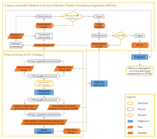
Figure 1.
Technical flowchart.

Table 1.
Configuration of the computer in this research.
2.1. Study Area and Data
The GF-2 image, reference polygons, and ground verification photos and their locations are shown in Figure 2, among which the original images and photos are the same as those of a study by Yao et al. [29], while the reference polygons were improved manually through visual interpretation in some places. For instance, because the imaging time of the GF-2 image is earlier than that of the photo in Figure 2a, the weeds and shrubs that covered the PG with walls in the photo do not appear on the GF-2 image; thus, a PG with walls was added to the new reference polygons. PGs both with and without walls [26], and water, trees, buildings with high reflectance, residences, and barren land, are contained in the study area, which is a typical one in Shouguang City, Shandong Province, China. As a footnote, Table 2 presents basic parameters of the GF-2 images in this study [38].
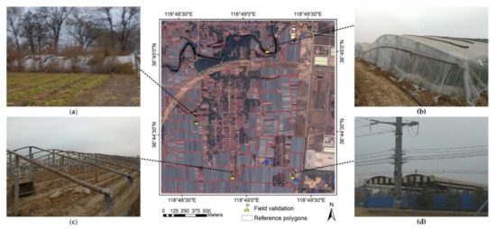
Figure 2.
GF-2 image, reference polygons and ground verification photos of the experimental area: (a) PG with walls; (b) PGs without walls with higher reflectance in image; (c) unsheathed PGs without walls; (d) other sheds used for storage.
Table 2.
Band no., spectral range, spatial resolution, and bit depth of GF-2 images.
2.2. Preprocessing of GF-2 Images
Three schemes were designed for the comparative experiments: the first was used to generate the control group, and the other two were used to generate experimental groups. All preprocessing operations were conducted in ENVI (L3Harris Geospatial Solutions, Inc., Broomfield, CO, USA) software.
2.2.1. Orthographical Correction, Image Registration and Fusion
Firstly, we orthorectified the GF-2 images using rational polynomial coefficients and ASTER GDEM version 2 [39]; secondly, we registered the multispectral image without atmospheric correction (MI) to the panchromatic image that is only orthorectified, and then fused them using the Gram Schmidt Pan Sharpening tool, which outperforms most of the other pan sharpening methods in terms of both maximizing image sharpness and minimizing color distortion [40,41]; thus, a multispectral and panchromatic fusion image without atmospheric correction (FI) with 0.8 m resolution could be obtained.
2.2.2. Atmospheric and Orthographical Correction, Image Registration and Fusion
The difference between this schedule and the first one is the radiometric calibration and atmospheric correction prior to the orthographical correction; thus, an atmospheric-corrected multispectral image (ACMI) with 3.2 m resolution and an atmospheric-corrected fusion image (ACFI) with 0.8 m resolution can be obtained. The atmospheric correction was conducted using the Fast Line-of-sight Atmospheric Analysis of Spectral Hypercubes (FLAASH) [42].
2.2.3. Image Enhancement
Linear compression is a concept opposite to linear stretching. The uniform expansion of the image gray value is called linear stretching, whereas the uniform reduction is called linear compression. The maximum digital number (MDN) value is the maximum gray value of a single-band image in a monochrome or multispectral image, and the gray value of each pixel in each band can be reassigned between 0 and MDN according to the frequency of each original gray value, thereby changing the distribution range of the gray value. When the MDN is reduced, the gray values of the pixels in the image will be compressed to a smaller range [43]. The MDNs adopted in this study were 511, 255, and 127.
Spatial filtering is also an important method for enhancing image information by changing the DN value of an image for a specific purpose. In order to further improve the heterogeneity among pixels and reduce the noise, the input image is filtered from the spatial domain (x, y) and the spatial frequency domain (ξ, η), respectively [43,44]. In this study, mean Gaussian low-pass (GLP) and median convolution filters with a size of 3 × 3 were selected in the spatial domain, and the circular low-pass (CLP) filter combined with FFT was selected in the spatial frequency domain.
2.3. MRS via ESP 2 Tool
Focusing on the effect of atmospheric correction and image enhancement on MRS, the uniform shape and compactness were set as 0.3 and 0.5, respectively [29]. Thus, each optimal scale parameter (OSP) in this research was automatically calculated using the ESP 2 tool [33] with the algorithm parameters [29] set as shown in Table 3. Level 1 and its segments in the exported results were adopted for the next stage of analysis.
Table 3.
Algorithm parameters and settings in the ESP 2 tool.
2.4. A Semi-Automatic Method to Extract EPGSs
The automatic extraction of EPGSs from different segmentation results requires different object samples, features, parameters, and thresholds, which is cumbersome and makes it difficult to avoid the error of false extraction and omission. In this study, the EPGSs were extracted by a semi-automatic process.
Firstly, the point samples used to select PG segments were made, and then the segments that intersected with the point samples were automatically extracted as the PG segments by the eCognition classification algorithm. Finally, visual interpretation and manual selection were carried out to extract the EPGSs. The geometric error of manual selection results has a theoretical minimum, but the error of total extraction area does not, because the total extraction area will be close to the real area of the PGs when the omission error is close to the false error.
2.4.1. Production of Point Samples
Segments overlapping with the reference polygons can be quickly classified using the assign algorithm in eCognition; however, the PG pixel proportion of the segments classified by the boundary of reference polygons is often less than 50%. In order to improve the efficiency of visual interpretation, this study first segmented the GF-2 image by using a chessboard segmentation algorithm combined with the reference polygons (Figure 3a). Thus, the segments that intersected with the reference polygons were classified as initial samples and, then, we discarded most of the segment samples that were located at the boundary of the reference polygons by area calculation and filtering (Figure 3b). Finally, the point samples used for extracting PG segments could be derived using the export algorithm in eCognition (Figure 3c), and the “center of gravity” type was chosen when exporting them.
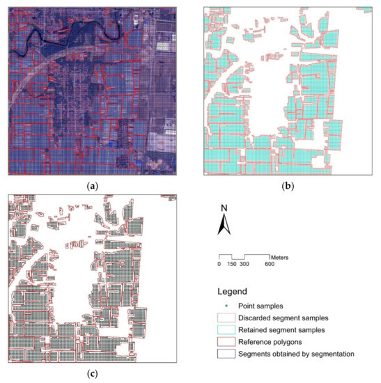
Figure 3.
Production of point samples based on reference polygons: (a) chessboard segmentation combined with reference polygons; (b) discarded and retained segment samples after filtering; (c) relationship between point samples and reference polygons.
In this study, the size of the chessboard was set as 10 pixels or 20 pixels according to the characteristics of the PG segments. For the segmentation results with a large number of segments and a small average area, a denser chessboard was used; otherwise, we used a sparser one. Figure 4 shows the specific algorithm steps of making point samples based on reference polygons and a chessboard with 20 pixels as an example.
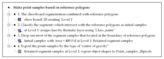
Figure 4.
Algorithm for making point samples.
2.4.2. Criterion for Determining EPGSs
In a broad sense, the PG segment refers to all the segments containing PG pixels when the characteristics of non-PG pixels are not obvious. If the proportion of PG pixels in these segments form a finite set G = {g1, g2, …, gi, …}, then PG segments with g above or equal to a set value gset (g ≥ gset) can be defined as EPGSs, in which the patches composed of non-PG pixels can be called extra fragments (EF), which are treated as false errors in the subsequent analysis. Moreover, those segments with g < gset can be regarded as invalid PG segments in a narrow sense, and the patches composed of PG pixels can be called lost fragments (LF), which are treated as omission errors in the subsequent analysis.
Generally speaking, the boundary of PG segments cannot completely coincide with the reference polygons. Supposing that the total area of EPGSs is S, and the total area of corresponding reference polygons is R, the area of extra fragments is EF, and the area of lost fragments is LF. For a specific segmentation result, with the gset decreasing, EF will increase, while LF will decrease accordingly. When g = gmin, the area of EPGSs reaches the maximum value Smax, EF and the difference between S and R reaches the maximum value EFmax = Smax− R, while LF reaches the minimum value LFmin = 0 and the producer accuracy (PA) reaches the maximum (PAmax = 1).
Conversely, with the gset increasing, EF will decrease, and LF will increase accordingly; so, when g = gmax, the area of EPGSs reaches the minimum value Smin, and EF reaches the minimum value EFmin, while LF and the difference between S and R reaches the maximum value LFmax = R − Smin, and the PA reaches the minimum. In this process, because the numerator and denominator of the user accuracy will change at the same time, it is difficult to judge the g value corresponding to its maximum and minimum values.
According to the inference above, when different g values are used to extract the EPGSs in a specific segmentation result, EF and LF are in a trade-off relationship. From an application perspective, the reasonable gset value should make the difference between S and R (which is equal to the difference between EF and LF) close to 0. Since the higher the gset value, the more stringent the evaluation criterion [36], and when gset is set as 60%, EF is much higher than LF. If the gset is set too high (for example, 80%), many segments containing PG pixels will not be classified as EPGSs, which leads to LF being much higher than EF; hence, the value of gset can be set as 70%.
2.4.3. Extraction of EPGSs
Taking the extraction of EPGSs from FI as an example: Firstly, the point samples were used to obtain the segments that intersected with them (Figure 5a). Then, a small number of segments that did not qualify with “above or equal 70% pixels belonging to the PG” were discarded; hence, the retained PG segments were those needed in the subsequent analysis. Moreover, a few omitted segments that did not intersect with point sample points but satisfied the criterion were added as the EPGSs (Figure 5b).
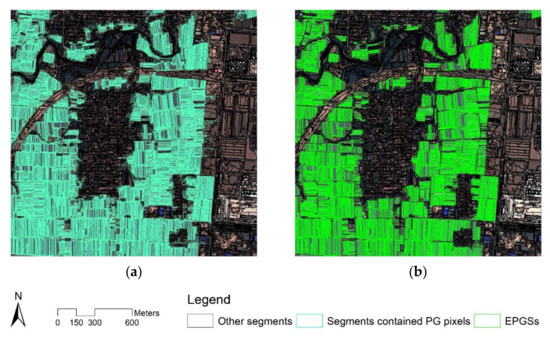
Figure 5.
Extracting EPGSs from FI based on point samples: (a) segments intersecting with point samples; (b) EPGSs.
2.5. Evaluation System
According to the single variable principle, all MRS times T in this study were obtained off-line with the running of a single program. In order to evaluate the rationality of the experimental settings, intersection over union (IoU) was used to preliminarily evaluate the accuracy of EPGSs, and then the OSI-USI-ETA-CEI pattern [29] was used to evaluate the segmentation error. In order to facilitate comparison, the value of 1 − IoU was taken as the evaluation parameter for subsequent analysis. The description or expression of each parameter is shown in Table 4.
Table 4.
The description or expression of evaluation parameters.
In the formula, the set S represents the total area of EPGSs, and the set R represents the total area of reference polygons; v represents the number of EPGSs of the optimal segmentation result obtained by the ESP 2 tool, and v1 specifically refers to the number of EPGSs in the fusion image without atmospheric correction in the study area. The higher the OSI value, the heavier the over-segmentation degree. The sets LF and EF represent the total area of lost fragments and extra fragments of EPGSs, respectively; the higher the USI, the greater the error of under-segmentation, and the higher the ETA value, the greater the error of the total area. Regarding the CEI, λ is used to rescale the value of quantity-based OSI so that the indicator will not overwhelm the value of area-based USI and ETA.
3. Results
3.1. Contrast Experiment
As a comparative experiment, the segmentation evaluation parameters of FI can be obtained as shown in Table 5.
Table 5.
Segmentation evaluation parameters of fusion image without atmospheric correction.
3.2. Effect of Atmospheric Correction on EPGSs of MI
After the MRS via ESP 2 tool, the segmentation and EPGSs extraction results of the multispectral image without atmospheric correction (MI) and the atmospheric-corrected multispectral image (ACMI) were obtained. These results are shown in Figure 6 and the relevant parameters are presented in Table 6.
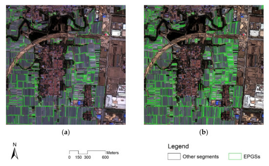
Figure 6.
Comparison of EPGSs of MI and ACMI: (a) MI; (b) ACMI.
Table 6.
Comparison of segmentation evaluation parameters of MI and ACMI.
It can be seen from Table 6 that, compared with MI, both the OSP and T of ACMI had a small increase, and the values of v and OSI increased significantly, indicating that the atmospheric correction can increase the heterogeneity of DN values of GF-2 multispectral image. The values of USI, ETA, and CEI decreased by 0.032, 0.043, and 0.066, respectively, indicating that the atmospheric correction can significantly improve the quality of EPGSs of GF-2 multispectral image, which is consistent with the hypothesis, although the value of USI still has significant room for improvement.
3.3. Effect of Linear Compression and Mean Filtering on EPGSs of ACFI
Firstly, ACFI was enhanced to obtain compressed floating format images with MDNs of 511, 255, and 127, and, then, the DN values of the four images were filtered in turn using the mean filter with 3 × 3; thus, seven derivative images were obtained, and their segmentation and EPGSs extraction results are shown in Figure 7, while the relevant parameters appear in Table 7.
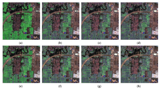
Figure 7.
Effects of linear compression and mean filtering on EPGSs of ACFI: (a) MDN initial; (b) MDN 511; (c) MDN 255; (d) MDN 127; (e) MDN initial and mean 3 × 3; (f) MDN 511 and mean 3 × 3; (g) MDN 255 and mean 3 × 3; (h) MDN 127 and mean 3 × 3.
Table 7.
Effects of linear compression and mean filtering on segmentation evaluation parameters of ACFI.
As shown in Figure 7 and Table 7, the number of EPGSs in the experimental area significantly reduced after linear compression or mean filtering, which is more conducive to feature analysis and algorithm extraction.
By analyzing Table 5 and Table 7, it can be found that, compared with FI, the OSP and OSI of ACFI increased by 45 and 0.188, respectively. This further shows that the nonlinear stretching of the image DN value by atmospheric correction increases the heterogeneity between pixels and leads to an increase in the number of EPGSs. Nevertheless, the values of 1 − IoU, USI, and CEI of ACFI decreased by 0.011, 0.018, and 0.017, respectively, and the change in ETA was close to 0. Hence, the atmospheric correction in this study is conducive to improving the accuracy of the segmentation boundary, which lays the foundation for continuing to use image enhancement to improve the quality of EPGSs. By visualizing the relevant parameters in Table 7, the comparison of OSP and T, IoU, and 1 − IoU, and the OSI-USI-ETA-CEI pattern, can be obtained, as shown in Figure 8.
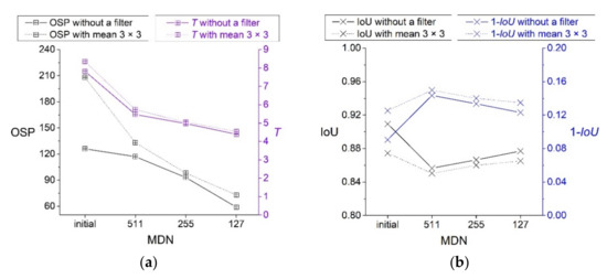
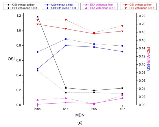
Figure 8.
Effects of linear compression and mean filtering on segmentation evaluation parameters of ACFI: (a) OSP and segmentation time; (b) IoU and 1 − IoU; (c) OSI-USI-ETA-CEI pattern.
It can be seen from Table 7 and Figure 8 that, compared with the case without image enhancement, when the DN value of ACFI is linearly compressed to MDN 511, 255, and 127, the OSP and the segmentation time T (Figure 8a) can be significantly reduced, because the reduction in the DN value of the image reduces the calculation amount of MRS, and thus increases the computational efficiency of the software. Moreover, the values of 1 − IoU and USI increased first and then decreased gradually, and the values of ETA were close to 0, while the values of OSI and CEI decreased first and then increased slightly. Hence, the minimal value of CEI in the experiment was 0.176 when the DN value of ACFI was linearly compressed to 0–255.
When the mean filter with 3 × 3 was used on the linearly compressed ACFI, the OSI was lower than that without a filter, but OSP, T, 1 − IoU, USI, and CEI were increased, indicating that a mean filter with a size of 3 × 3 will reduce the segmentation quality when it is used to enhance the linearly compressed ACFI.
3.4. Effect of Spatial Filtering on EPGSs of ACFI Compressed to MDN 255
In order to improve the segmentation quality based on ACFI compressed to MDN 255, a Gaussian low-pass (GLP) and median convolution filter in the spatial domain, and a circular low-pass (CLP) filter in the spatial frequency domain, were applied. The sizes of GLP and median filter were also set to 3 × 3, while the standard deviation of GLP filter was 0.375, as calculated by dividing the kernel size into 8. Moreover, the radius size of the CLP filter was tested with 1000, 900, 800, and 700 pixels according to the image size. The experimental results are shown in Figure 9 and Table 8.
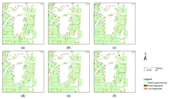
Figure 9.
Effects of spatial filtering on PG extraction results of ACFI compressed to MDN 255: (a) GLP 3 × 3; (b) median 3 × 3; (c) CLP 1000; (d) CLP 900; (e) CLP 800; (f) CLP 700.
Table 8.
Effects of spatial filtering on segmentation evaluation parameters of compressed ACFI.
As shown in Figure 9, the EF of each filtering experiment is mainly distributed on the roads adjacent to the greenhouses, while the distribution areas of the LF include many scattered PGs in addition to the roads. Therefore, it is possible extract the roads first or use the existing information about the road to improve segmentation quality in a follow-up study.
Combining the relevant data in Table 7 and Table 8, the relevant parameters can be organized into the comparison chart shown in Figure 10. It can be seen from Figure 10a that, although the variation range of T in each scheme is small, it still shows strong consistency with the variation trend of dimensionless OSP.
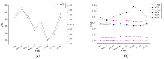
Figure 10.
Effects of spatial filtering on segmentation evaluation parameters of ACFI compressed to MDN 255: (a) OSP and segmentation time; (b) segmentation evaluation parameters.
As shown in Figure 10b, although the change trend of OSI is opposite to that with 1 − IoU, USI, and CEI, and the range is larger, the change range of λ × OSI and ETA is small, and the values of ETA are close to 0. Thus, the change trend of CEI and USI is consistent, which suggests that the CEI in the comparative experiment is mainly affected by USI. In general, all the spatial filtering schemes in this study other than the mean filter have a CEI that is lower than 0.176, which is the minimal CEI of compressed ACFI without a filter. Thus, the optimal preprocessing scheme of the study area is to linearly compress the DN value of ACFI to 0–255, and then use FFT and a circular low-pass filter with a radius size of 800 pixels for filtering in the spatial frequency domain. By applying this scheme, the CEI has a minimum value of 0.159.
4. Discussion
4.1. Comparison of IoU and OSI-USI-ETA-CEI Pattern
Since the IoU is widely applied, the consistent trend of 1 − IoU and USI in Figure 8 and Figure 10 illustrates the validity of USI. However, the IoU cannot indicate the variation in the degree of over-segmentation, nor the change trend of the difference between S and R, whereas the OSI and the ETA can do that, respectively. Thus, the OSI-USI-ETA-CEI pattern can be more effective than IoU when it is needed to evaluate the quality of EPGSs.
4.2. Comparison with Related Research
For comparison, Yao et al. obtained the lowest CEI of 0.185 using the image enhancement method of gray compression and mean filtering on the fusion image without atmospheric correction in the same area [29]. Even though the criterion of EPGS (the proportion of PG pixels in the segment) was raised from 60% to 70%, the CEI of nine atmospheric correction and image enhancement schemes in this study was lower than 0.185. The main reasons for the improvement are the use of atmospheric correction to optimize the DN value of the image, the use of new filters, and the point samples, which were made by improved reference polygons, which improved the extraction efficiency and accuracy of the EPGSs.
4.3. Hypothesis of Why Atmospheric Correction and Image Enhancement Works
From the results in Section 3, it is suggested that not only the CEIs of ACMI and ACFI, but also those of the linearly compressed ACFI, are lower than that of the MI, FI, and ACFI, respectively. In order to find the reason for this, the line and symbol plots shown in Figure 11 were obtained by counting the pixel number of each DN interval of the blue bands of MI, ACMI, FI, and ACFI.
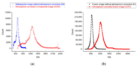
Figure 11.
Effect of atmospheric correction on DN value of multispectral images and fusion images: (a) multispectral images; (b) fusion images.
It can be seen from Figure 11a that atmospheric correction has the effect of expanding the DN value range of the MI, which can be regarded as the nonlinear stretching of the DN value. Since the radiometric calibration process also stretches the DN value of the panchromatic image, the DN value range of ACFI is significantly higher than that of the fusion image without atmospheric correction (Figure 11b). Combined with the increase in OSIs and the decrease in USIs, it is suggested that atmospheric correction can improve the heterogeneity between the PG pixels and non-PG pixels; thus, the CEIs of ACMI and ACFI are lower than those of MI and FI, respectively.
Alternatively, since the ACFI can easily lead to over-segmentation, the linearly compressed ACFI can obtain better segmentation results by decreasing the heterogeneity of the whole image.
Regarding filters, whether they help improve the quality of EPGSs is still determined by heterogeneity, since the filters can remove image noise, while the homogeneity between the PG pixels and non-PG pixels can be increased at the same time.
Therefore, a hypothesis can be inferred combined with the theory of MRS that, if the increase in heterogeneity between the PG pixels and non-PG pixels is greater than that of the homogeneity during image preprocessing, then the quality of EPGSs will increase; otherwise, it will decrease.
4.4. Next Steps
Limited by the experimental conditions, this research only analyzed the effects of atmospheric correction on EPGSs of GF-2 multispectral image, and the effects of atmospheric correction, linear compression, and spatial filtering on EPGSs of GF-2 fusion image in the study area. Other image correction and enhancement methods or segmentation algorithms to improve the quality of EPGSs in the study area or other areas can be further discussed in a follow-up study.
PGs in China can be divided into two kinds according to whether they are built with walls [26]. However, some research has mistakenly identified PGs with walls as PGs without walls. For instance, Figure 7 in the study of Ma et al. [10] mistakenly matches a photograph of PGs without walls to the satellite image of PGs with walls, which can be very misleading to the reader. It is essential to distinguish the two main types of PG, both in field investigation and image interpretation, in addition to the extraction.
In order to extract the surface object from various satellite images with better accuracy, many kinds of machine learning models have been applied in computing [45,46], which are also worthy of being assessed adequately in subsequent PG extraction.
5. Conclusions
The main conclusions are as follows:
- Through chessboard segmentation combined with reference polygons, in addition to filtering and exporting, boundary-removed point samples with adjustable density can be made to improve the accuracy and efficiency of PG segment extraction, and lay the data foundation for comparative experiments under control variables.
- With the control of experimental variables, the OSP and segmentation time showed a consistent trend, which indicates the stability of the ESP 2 tool. Moreover, OSI, USI, and CEI all showed obvious rules, and the values of ETA were close to 0, indicating that the proportion of 70% designed in the experiment is a reasonable gset value.
- The OSI-USI-ETA-CEI pattern can be more effective than IoU when it is needed to evaluate the quality of EPGSs of GF-2 images in the study area.
- The CEIs of the EPGSs of ACMI and ACFI, and of the enhanced ACFI, have lower values than the control groups. This illustrates the rationality of the experiment. Moreover, the atmospheric correction and image enhancement, with heterogeneity and target characteristics taken into account prior to segmentation, are helpful in improving the quality of EPGSs of GF-2 images in the study area.
- Even though the mean filter with a size of 3 × 3 did not improve the quality of EPGSs of the linearly compressed ACFI, in this study, the filter of GLP and median, and the filter of CLP after FFT, improved the quality of EPGSs of ACFI with MDN compressed to 255. Of these, the CLP filter with a radius of 800 pixels obtained the lowest CEI in this study.
Author Contributions
Conceptualization, Yao Yao; Data curation, Yao Yao; Formal analysis, Yao Yao; Funding acquisition, Shixin Wang; Investigation, Yao Yao; Methodology, Yao Yao; Project administration, Shixin Wang; Software, Yao Yao; Supervision, Shixin Wang; Validation, Yao Yao; Visualization, Yao Yao; Writing—original draft, Yao Yao; Writing—review and editing, Yao Yao. All authors have read and agreed to the published version of the manuscript.
Funding
This research was funded by National Key Research and Development Program of China grant number 2021YFB3901201.
Institutional Review Board Statement
Not applicable.
Informed Consent Statement
Not applicable.
Data Availability Statement
The data presented in this study are available on request from the authors.
Acknowledgments
We thank the China Center for Resources Satellite Data and Application for providing the GF-2 images. We thank Futao Wang and Wenliang Liu for their funding support on this research. We thank Fuli Yan, Hongjie Wang and Yumin Gu for their assistance with the field validation.
Conflicts of Interest
The authors declare no conflict of interest.
Abbreviations
The following abbreviations are used in this article:
| MRS | Multi-Resolution Segmentation |
| PG | Plastic Greenhouse |
| GF-2 | Gaofen-2 |
| EPGSs | Effective Plastic Greenhouse Segments |
| IoU | Intersection over Union |
| OSI | Over-Segmentation Index |
| USI | Under-Segmentation Index |
| ETA | Error index of Total Area |
| CEI | Composite Error Index |
| ESP | Estimation of Scale Parameter |
| OSP | Optimal Scale Parameter |
| ED2 | Euclidean Distance 2 |
| FFT | Fast Fourier Transform |
| CLP | Circular Low-Pass |
| MI | Multispectral Image without atmospheric correction |
| FI | Fusion Image without atmospheric correction |
| ACMI | Atmospheric-Corrected Multispectral Image |
| ACFI | Atmospheric-Corrected Fusion Image |
| EF | Extra Fragments |
| LF | Lost Fragments |
| MDN | Maximum Digital Number |
| GLP | Gaussian Low-Pass |
References
- Jiménez-Lao, R.; Aguilar, F.J.; Nemmaoui, A.; Aguilar, M.A. Remote Sensing of Agricultural Greenhouses and Plastic-Mulched Farmland: An Analysis of Worldwide Research. Remote Sens. 2020, 12, 2649. [Google Scholar] [CrossRef]
- Yang, D.; Chen, J.; Zhou, Y.; Chen, X.; Chen, X.; Cao, X. Mapping plastic greenhouse with medium spatial resolution satellite data: Development of a new spectral index. ISPRS J. Photogramm. Remote Sens. 2017, 128, 47–60. [Google Scholar] [CrossRef]
- Zhang, P.; Du, P.; Guo, S.; Zhang, W.; Tang, P.; Chen, J.; Zheng, H. A novel index for robust and large-scale mapping of plastic greenhouse from Sentinel-2 images. Remote Sens. Environ. 2022, 276, 113042. [Google Scholar] [CrossRef]
- Shi, L.; Huang, X.; Zhong, T.; Taubenbock, H. Mapping Plastic Greenhouses Using Spectral Metrics Derived From GaoFen-2 Satellite Data. IEEE J. Sel. Top. Appl. Earth Obs. Remote Sens. 2020, 13, 49–59. [Google Scholar] [CrossRef]
- Hasituya; Chen, Z.; Wang, L.; Wu, W.; Jiang, Z.; Li, H. Monitoring Plastic-Mulched Farmland by Landsat-8 OLI Imagery Using Spectral and Textural Features. Remote Sens. 2016, 8, 353. [Google Scholar] [CrossRef]
- Yu, B.; Song, W.; Lang, Y. Spatial Patterns and Driving Forces of Greenhouse Land Change in Shouguang City, China. Sustainability 2017, 9, 359. [Google Scholar] [CrossRef]
- Ou, C.; Yang, J.; Du, Z.; Liu, Y.; Feng, Q.; Zhu, D. Long-Term Mapping of a Greenhouse in a Typical Protected Agricultural Region Using Landsat Imagery and the Google Earth Engine. Remote Sens. 2019, 12, 55. [Google Scholar] [CrossRef]
- Ou, C.; Yang, J.; Du, Z.; Zhang, T.; Niu, B.; Feng, Q.; Liu, Y.; Zhu, D. Landsat-Derived Annual Maps of Agricultural Greenhouse in Shandong Province, China from 1989 to 2018. Remote Sens. 2021, 13, 4830. [Google Scholar] [CrossRef]
- Lin, J.; Jin, X.; Ren, J.; Liu, J.; Liang, X.; Zhou, Y. Rapid Mapping of Large-Scale Greenhouse Based on Integrated Learning Algorithm and Google Earth Engine. Remote Sens. 2021, 13, 1245. [Google Scholar] [CrossRef]
- Ma, A.; Chen, D.; Zhong, Y.; Zheng, Z.; Zhang, L. National-scale greenhouse mapping for high spatial resolution remote sensing imagery using a dense object dual-task deep learning framework: A case study of China. ISPRS J. Photogramm. Remote Sens. 2021, 181, 279–294. [Google Scholar] [CrossRef]
- Chen, W.; Xu, Y.; Zhang, Z.; Yang, L.; Pan, X.; Jia, Z. Mapping agricultural plastic greenhouses using Google Earth images and deep learning. Comput. Electron. Agric. 2021, 191, 106552. [Google Scholar] [CrossRef]
- Zhang, X.; Cheng, B.; Chen, J.; Liang, C. High-Resolution Boundary Refined Convolutional Neural Network for Automatic Agricultural Greenhouses Extraction from GaoFen-2 Satellite Imageries. Remote Sens. 2021, 13, 4237. [Google Scholar] [CrossRef]
- Feng, Q.; Niu, B.; Chen, B.; Ren, Y.; Zhu, D.; Yang, J.; Liu, J.; Ou, C.; Li, B. Mapping of plastic greenhouses and mulching films from very high resolution remote sensing imagery based on a dilated and non-local convolutional neural network. Int. J. Appl. Earth Obs. Geoinf. 2021, 102, 102441. [Google Scholar] [CrossRef]
- Chen, D.; Zhong, Y.; Ma, A.; Cao, L. Dense Greenhouse Extraction in High Spatial Resolution Remote Sensing Imagery. In Proceedings of the IGARSS 2020—2020 IEEE International Geoscience and Remote Sensing Symposium, Waikoloa, HI, USA, 26 September–2 October 2020; pp. 4092–4095. [Google Scholar]
- Li, M.; Zhang, Z.; Lei, L.; Wang, X.; Guo, X. Agricultural Greenhouses Detection in High-Resolution Satellite Images Based on Convolutional Neural Networks: Comparison of Faster R-CNN, YOLO v3 and SSD. Sensors 2020, 20, 4938. [Google Scholar] [CrossRef]
- Jakab, B.; van Leeuwen, B.; Tobak, Z. Detection of Plastic Greenhouses Using High Resolution Rgb Remote Sensing Data and Convolutional Neural Network. J. Environ. Geogr. 2021, 14, 38–46. [Google Scholar] [CrossRef]
- Bektas Balcik, F.; Senel, G.; Goksel, C. Object-Based Classification of Greenhouses Using Sentinel-2 MSI and SPOT-7 Images: A Case Study from Anamur (Mersin), Turkey. IEEE J. Sel. Top. Appl. Earth Obs. Remote Sens. 2020, 13, 2769–2777. [Google Scholar] [CrossRef]
- Aguilar, M.A.; Jiménez-Lao, R.; Aguilar, F.J. Evaluation of Object-Based Greenhouse Mapping Using WorldView-3 VNIR and SWIR Data: A Case Study from Almería (Spain). Remote Sens. 2021, 13, 2133. [Google Scholar] [CrossRef]
- Aguilar, M.A.; Nemmaoui, A.; Novelli, A.; Aguilar, F.J.; García Lorca, A. Object-Based Greenhouse Mapping Using Very High Resolution Satellite Data and Landsat 8 Time Series. Remote Sens. 2016, 8, 513. [Google Scholar] [CrossRef]
- Aguilar, M.A.; Aguilar, F.J.; García Lorca, A.; Guirado, E.; Betlej, M.; Cichon, P.; Nemmaoui, A.; Vallario, A.; Parente, C. Assessment of Multiresolution Segmentation for Extracting Greenhouses from Worldview-2 Imagery. ISPRS—Int. Arch. Photogramm. Remote Sens. Spat. Inf. Sci. 2016, XLI-B7, 145–152. [Google Scholar] [CrossRef]
- Novelli, A.; Aguilar, M.A.; Nemmaoui, A.; Aguilar, F.J.; Tarantino, E. Performance evaluation of object based greenhouse detection from Sentinel-2 MSI and Landsat 8 OLI data: A case study from Almería (Spain). Int. J. Appl. Earth Obs. Geoinf. 2016, 52, 403–411. [Google Scholar] [CrossRef]
- Aguilar, M.A.; Novelli, A.; Nemamoui, A.; Aguilar, F.J.; García Lorca, A.; González-Yebra, Ó. Optimizing Multiresolution Segmentation for Extracting Plastic Greenhouses from WorldView-3 Imagery. In Proceedings of the Intelligent Interactive Multimedia Systems and Services, Gold Coast, Australia, 20–22 May 2017; pp. 31–40. [Google Scholar]
- Cui, B.; Huang, W.; Ye, H.; Li, Z.; Chen, Q. Object-oriented greenhouse cantaloupe identification by remote sensing technology. In Proceedings of the 2021 9th International Conference on Agro-Geoinformatics (Agro-Geoinformatics), Shenzhen, China, 26–29 July 2021; pp. 1–6. [Google Scholar]
- Feng, T.; Ma, H.; Cheng, X. Greenhouse Extraction from High-Resolution Remote Sensing Imagery with Improved Random Forest. In Proceedings of the IGARSS 2020—2020 IEEE International Geoscience and Remote Sensing Symposium, Waikoloa, HI, USA, 26 September–2 October 2020; pp. 553–556. [Google Scholar]
- Wu, C.; Deng, J.; Wang, K.; Ma, L.; Shah, T.A.R. Object-based classification approach for greenhouse mapping using Landsat-8 imagery. Int. J. Agric. Biol. Eng. 2016, 9, 79–88. [Google Scholar] [CrossRef]
- Nbs, C. Plan for the Third National Agricultural Census; China Statistics Press: Beijing, China, 2016. [Google Scholar]
- Agüera, F.; Aguilar, M.A.; Aguilar, F.J. Detecting greenhouse changes from QuickBird imagery on the Mediterranean coast. Int. J. Remote Sens. 2006, 27, 4751–4767. [Google Scholar] [CrossRef]
- Agüera, F.; Aguilar, F.J.; Aguilar, M.A. Using texture analysis to improve per-pixel classification of very high resolution images for mapping plastic greenhouses. ISPRS J. Photogramm. Remote Sens. 2008, 63, 635–646. [Google Scholar] [CrossRef]
- Yao, Y.; Wang, S. Evaluating the Effects of Image Texture Analysis on Plastic Greenhouse Segments via Recognition of the OSI-USI-ETA-CEI Pattern. Remote Sens. 2019, 11, 231. [Google Scholar] [CrossRef]
- Baatz, M.; Schäpe, A. Multiresolution segmentation: An optimization approach for high quality multi-scale image segmentation. In Proceedings of the Angewandte Geographische Informationsverarbeitung; Wichmann Verlag: Heidelberg, Germany, 2000; pp. 12–23. [Google Scholar]
- Ma, L.; Li, M.C.; Ma, X.X.; Cheng, L.; Du, P.J.; Liu, Y.X. A review of supervised object-based land-cover image classification. Isprs J. Photogramm. Remote Sens. 2017, 130, 277–293. [Google Scholar] [CrossRef]
- Coslu, M.; Sonmez, N.K.; Koc-San, D. Object-Based Greenhouse Classification from High Resolution Satellite Imagery: A Case Study Antalya-Turkey. ISPRS—Int. Arch. Photogramm. Remote Sens. Spat. Inf. Sci. 2016, XLI-B7, 183–187. [Google Scholar] [CrossRef]
- Dragut, L.; Csillik, O.; Eisank, C.; Tiede, D. Automated parameterisation for multi-scale image segmentation on multiple layers. ISPRS J. Photogramm. Remote Sens. 2014, 88, 119–127. [Google Scholar] [CrossRef] [PubMed]
- Martins, V.S.; Kaleita, A.L.; Gelder, B.K.; da Silveira, H.L.F.; Abe, C.A. Exploring multiscale object-based convolutional neural network (multi-OCNN) for remote sensing image classification at high spatial resolution. ISPRS J. Photogramm. Remote Sens. 2020, 168, 56–73. [Google Scholar] [CrossRef]
- Trimble. eCognition Developer 10.2 User Guide; Trimble: Sunnyvale, CA, USA, 2021. [Google Scholar]
- Marpu, P.R.; Neubert, M.; Herold, H.; Niemeyer, I. Enhanced evaluation of image segmentation results. J. Spat. Sci. 2010, 55, 55–68. [Google Scholar] [CrossRef]
- Liu, Y.; Bian, L.; Meng, Y.; Wang, H.; Zhang, S.; Yang, Y.; Shao, X.; Wang, B. Discrepancy measures for selecting optimal combination of parameter values in object-based image analysis. ISPRS J. Photogramm. Remote Sens. 2012, 68, 144–156. [Google Scholar] [CrossRef]
- CRESDA. GF-2. Available online: http://www.cresda.com/EN/satellite/7157.shtml (accessed on 5 November 2015).
- Tachikawa, T.; Hato, M.; Kaku, M.; Iwasaki, A. Characteristics of ASTER GDEM version 2. In Proceedings of the 2011 IEEE International Geoscience and Remote Sensing Symposium, Vancouver, BC, Canada, 24–29 July 2011; pp. 3657–3660. [Google Scholar]
- Laben, C.A.; Brower, B.V. Process for Enhancing the Spatial Resolution of Multispectral Imagery Using Pan-Sharpening. U.S. Patent 6011875, 4 January 2000. [Google Scholar]
- Maurer, T. How to pan-sharpen images using the gram-schmidt pan-sharpen method—A recipe. In Proceedings of the ISPRS Hannover Workshop, Hannover, Germany, 21–24 May 2013. [Google Scholar]
- Adler-Golden, S.; Berk, A.; Bernstein, L.; Richtsmeier, S.; Acharya, P.; Matthew, M.; Anderson, G.; Allred, C.; Jeong, L.; Chetwynd, J. FLAASH, a MODTRAN4 atmospheric correction package for hyperspectral data retrievals and simulations. In Proceedings of the 7th Ann. JPL Airborne Earth Science Workshop, Pasadena, CA, USA, 12–16 January 1998; pp. 9–14. [Google Scholar]
- Nixon, M.S.; Aguado, A.S. Feature Extraction & Image Processing for Computer Vision, 3rd ed.; Elservier and Pte Ltd.: Singapore, 2012. [Google Scholar]
- Lillesand, T.; Kiefer, R.W.; Chipman, J. Remote Sensing and Image Interpretation, 7th ed.; John Wiley & Sons: Hoboken, NJ, USA, 2015. [Google Scholar]
- Wang, X.; Zhang, J.; Xun, L.; Wang, J.; Wu, Z.; Henchiri, M.; Zhang, S.; Zhang, S.; Bai, Y.; Yang, S.; et al. Evaluating the Effectiveness of Machine Learning and Deep Learning Models Combined Time-Series Satellite Data for Multiple Crop Types Classification over a Large-Scale Region. Remote Sens. 2022, 14, 2341. [Google Scholar] [CrossRef]
- Anul Haq, M. Planetscope Nanosatellites Image Classification Using Machine Learning. Comput. Syst. Sci. Eng. 2022, 42, 1031–1046. [Google Scholar] [CrossRef]
Publisher’s Note: MDPI stays neutral with regard to jurisdictional claims in published maps and institutional affiliations. |
© 2022 by the authors. Licensee MDPI, Basel, Switzerland. This article is an open access article distributed under the terms and conditions of the Creative Commons Attribution (CC BY) license (https://creativecommons.org/licenses/by/4.0/).