
Multiscale Effects of Multimodal Public Facilities Accessibility on Housing Prices Based on MGWR: A Case Study of Wuhan, China


Abstract
:1. Introduction
2. Data and Methods
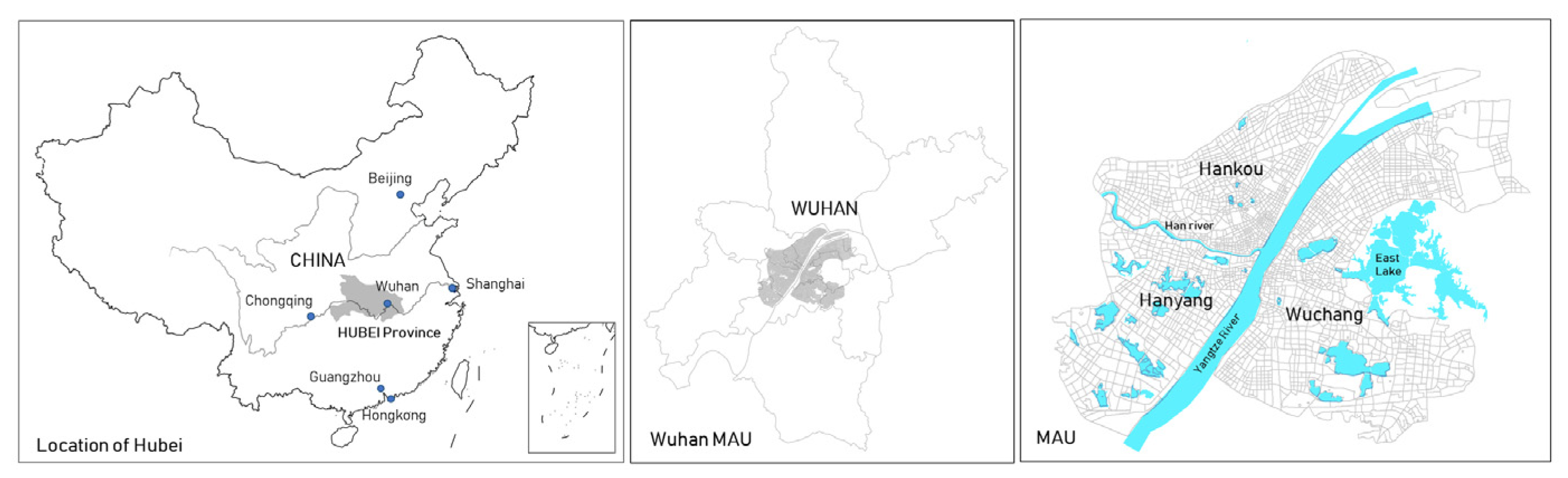
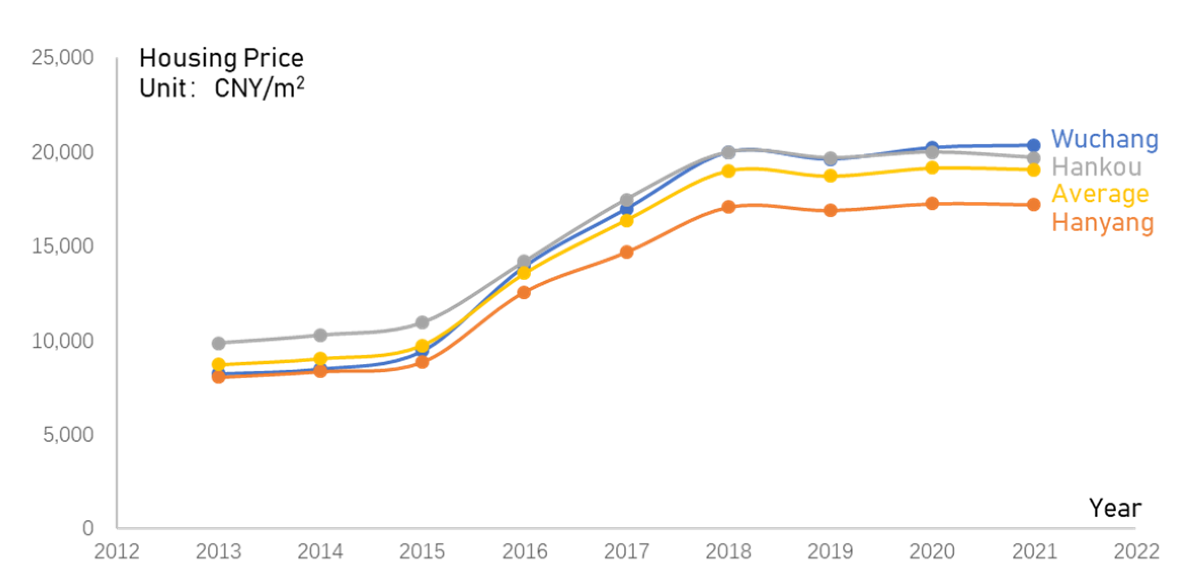
2.1. Study Area
2.2. Data Preprocessing
- (1)
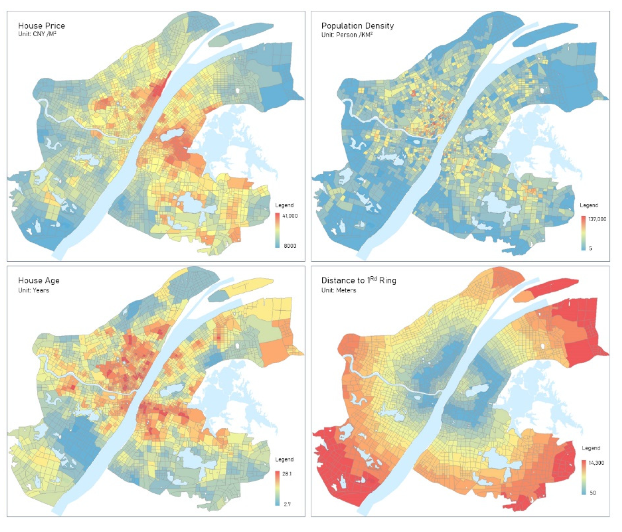
- Housing prices and average house age: the data were grasped from an online housing platform (Lianjia.com, accessed on 8 August 2021) in 2020, the mean value of all point-based housing price within the boundary of the TAZ was generated as the average value of each TAZ. In order to increase the comparability, the data set only retains the apartment type, the most mainstream residential form in China, and the villa is not included because of the scarcity and the extremely high price.
- (2)
- Public facilities: the data were extracted from the POI data of Baidu Maps, among which, only the public facilities often invested by the government was kept; education (kindergarten, elementary school, middle school), transportation (bus station, subway station), green space, hospital. Business and commercial spaces (stores, markets, offices) were also used for representing the employment centers. The hospitals have been further screened and only the general hospitals were retained. The corresponding accessibility of TAZ in the subsequent models were calculated based on the centroid of TAZ (n = 2383).
2.3. Methods
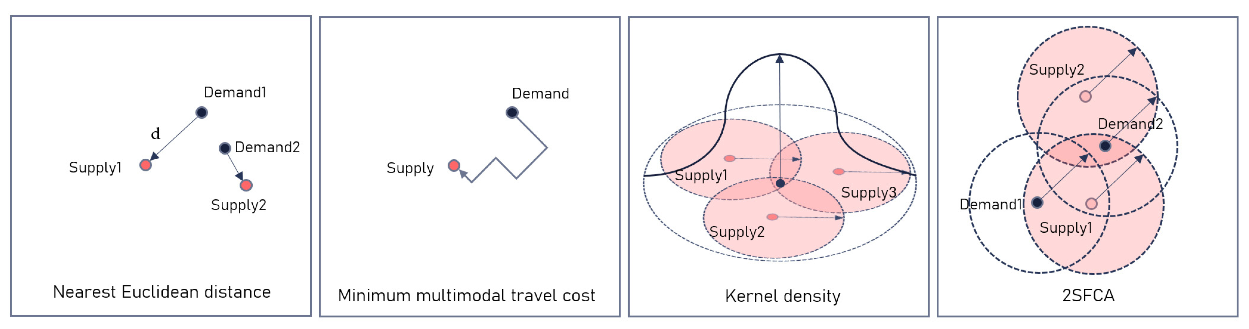
2.3.1. Multimodal Accessibility
- (1)
- Nearest Euclidean distance (NED)
- (2)
- Minimum multimodal travel cost (MMTC)
- (3)
- Kernel density (KD)
- (4)
- 2SFCA
2.3.2. Multiscale Geographical Weighted Regression
- (1)
- OLS Regression
- (2)
- Geographical Weighted Regression
- (3)
- Multiscale Geographical Weighted Regression:
3. Results
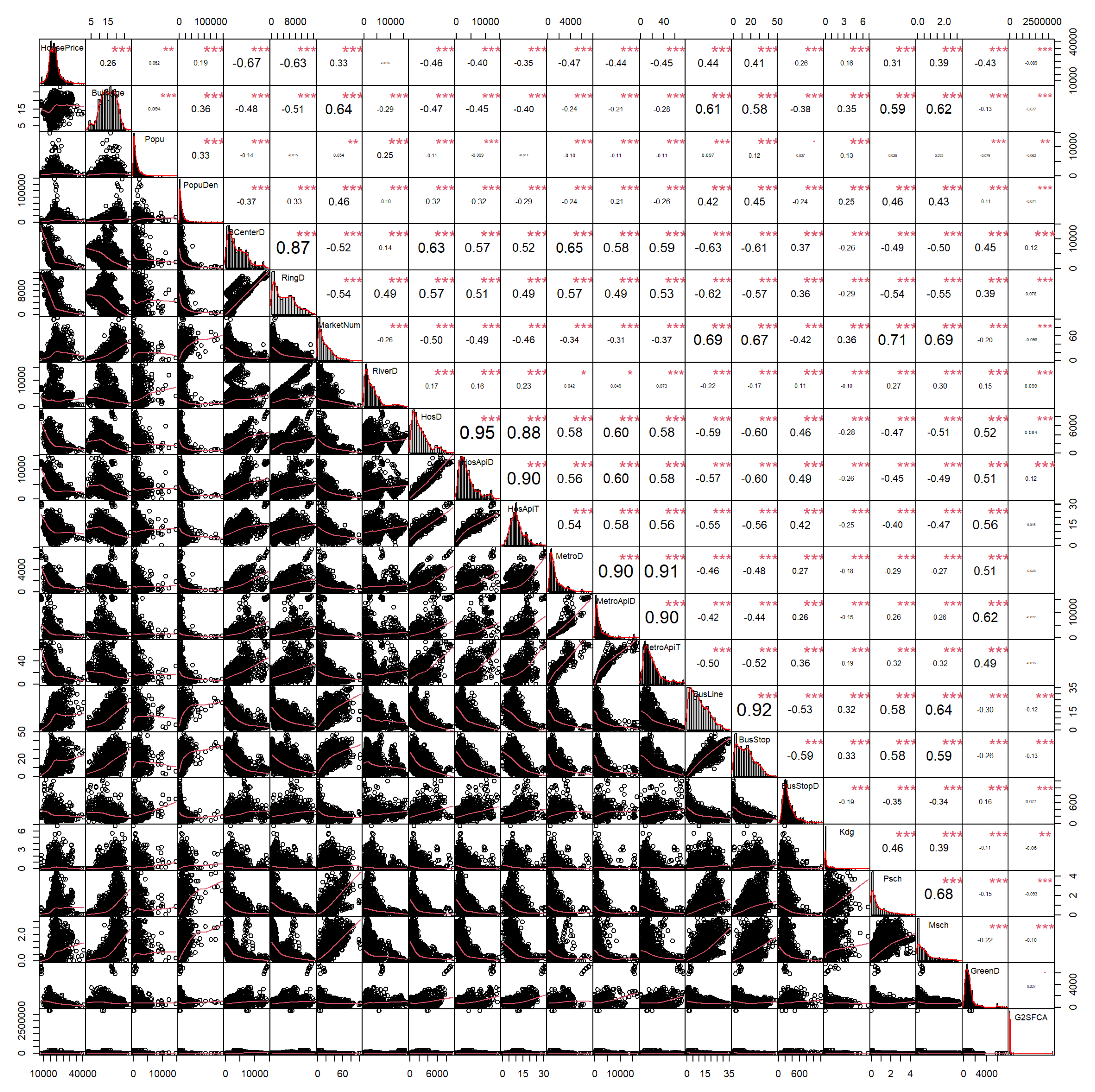
3.1. Preliminary Statistical Description and Correlation Test
3.2. OLS Regression
3.3. MGWR
3.3.1. Model Comparison
3.3.2. MGWR Parameter Estimates
3.3.3. Multiscale Effect of Multimodal Accessibilities
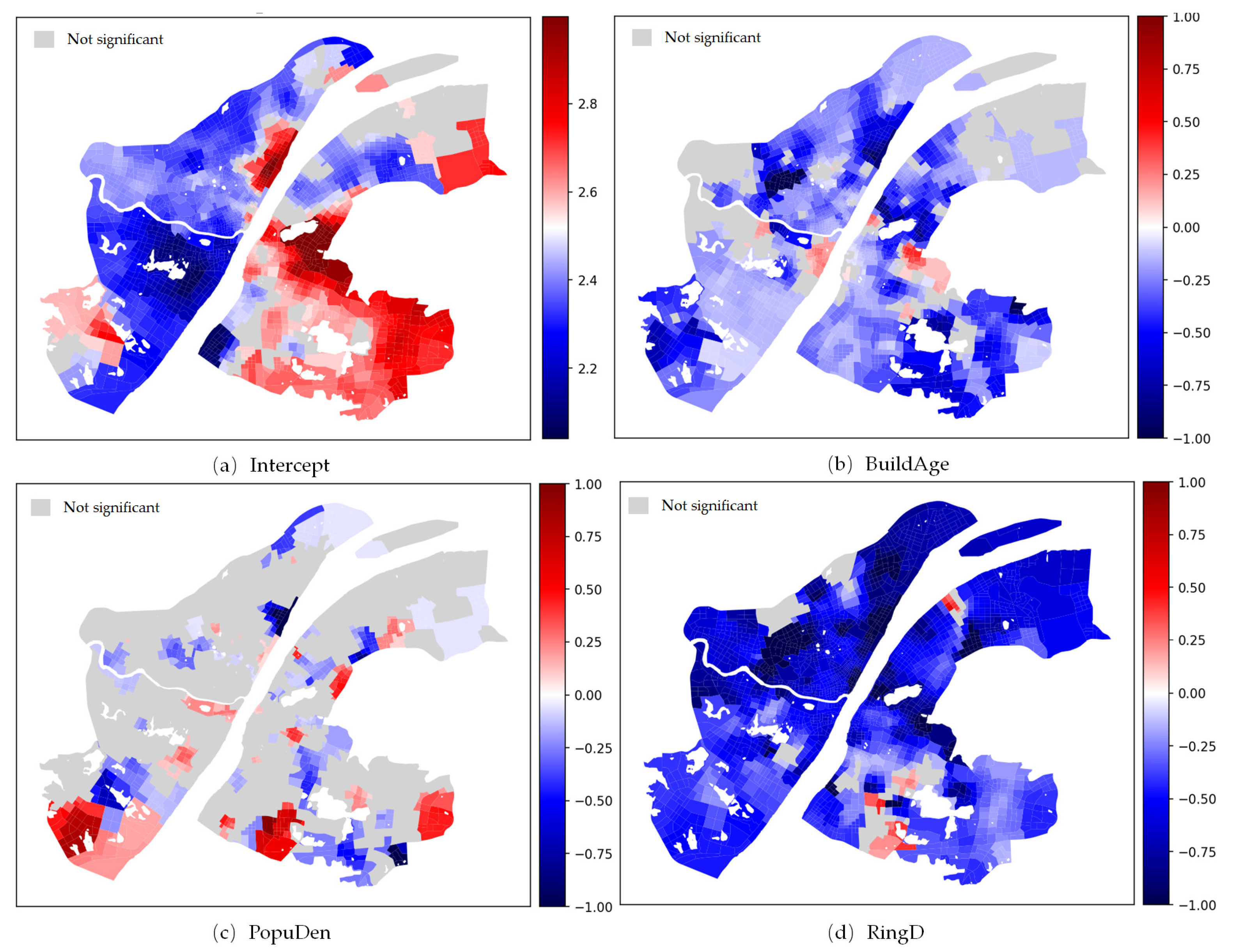
- (1)
- Intercept and control variables
- (2)
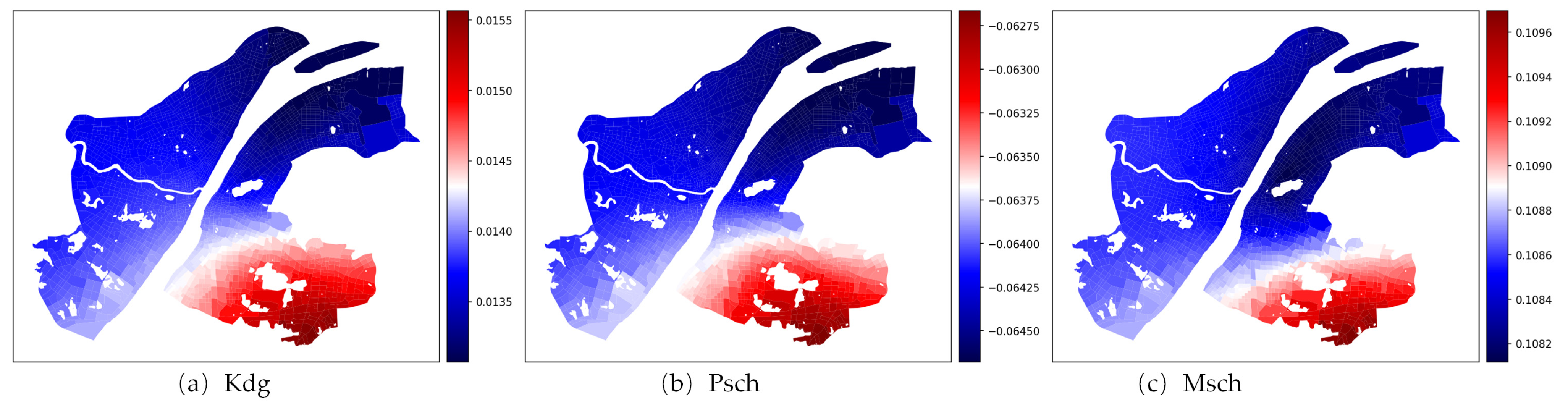
- Educational facilities
- (3)
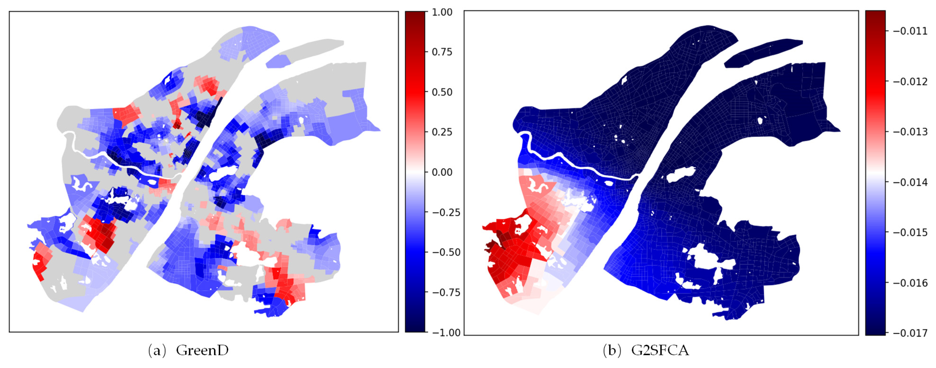
- Green space
- (4)
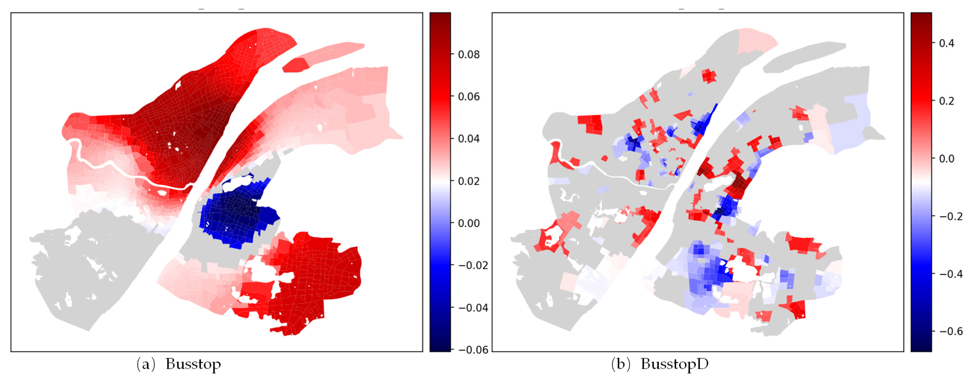
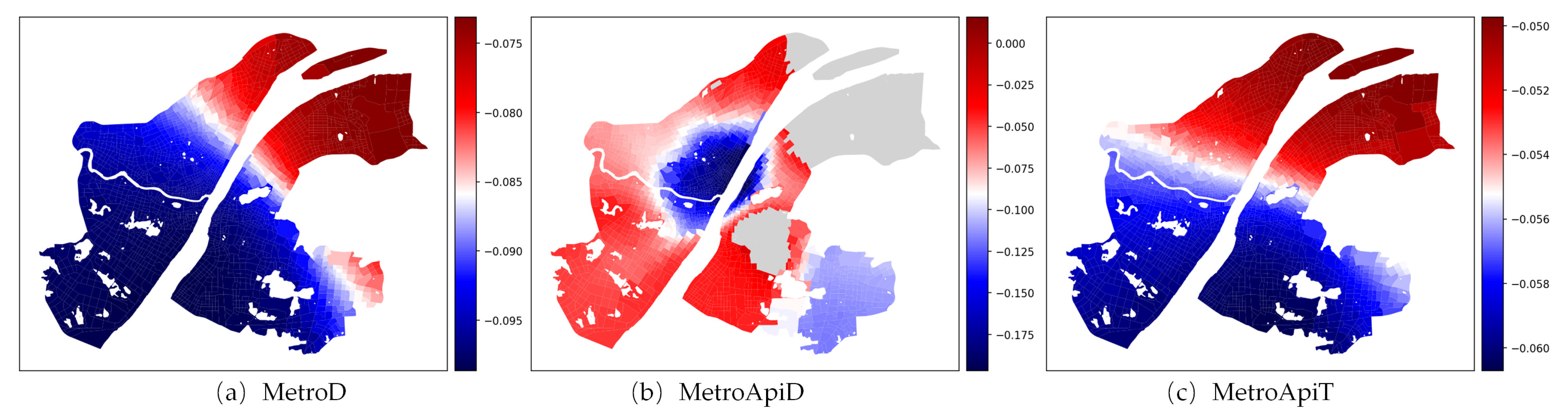
- Public transportation
- (5)
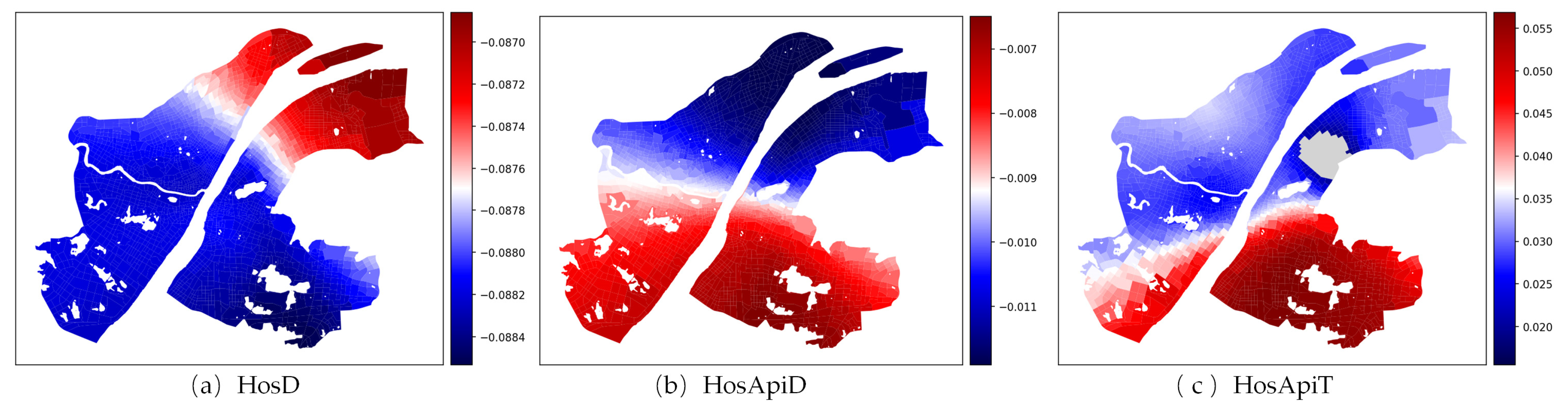
- Medical care facilities
4. Discussion
5. Conclusions
Author Contributions
Funding
Institutional Review Board Statement
Informed Consent Statement
Data Availability Statement
Conflicts of Interest
References
- Dadashpoor, H.; Rostami, F.; Alizadeh, B. Is inequality in the distribution of urban facilities inequitable? Exploring a method for identifying spatial inequity in an Iranian city. Cities 2016, 52, 159–172. [Google Scholar] [CrossRef]
- Rodriguez-Pose, A.; Storper, M. Housing, urban growth and inequalities: The limits to deregulation and upzoning in reducing economic and spatial inequality. Urban Stud. 2020, 57, 223–248. [Google Scholar] [CrossRef]
- Fransman, T.; Yu, D. Multidimensional poverty in South Africa in 2001–2016. Dev. S. Afr. 2019, 36, 50–79. [Google Scholar] [CrossRef] [Green Version]
- Wilson, D.; Bridge, G. School choice and the city: Geographies of allocation and segregation. Urban Stud. 2019, 56, 3198–3215. [Google Scholar] [CrossRef]
- Wolf, K.L.; Robbins, A.S.T. Metro Nature, Environmental Health, and Economic Value. Environ. Health Perspect. 2015, 123, 390–398. [Google Scholar] [CrossRef] [Green Version]
- Yang, L.; Zhou, J.; Shyr, O.F.; Huo, D. Does bus accessibility affect property prices? Cities 2019, 84, 56–65. [Google Scholar] [CrossRef]
- Zhao, C.; Nielsen, T.A.S.; Olafsson, A.S.; Carstensen, T.A.; Meng, X. Urban form, demographic and socio-economic correlates of walking, cycling, and e-biking: Evidence from eight neighborhoods in Beijing. Transp. Policy 2018, 64, 102–112. [Google Scholar] [CrossRef]
- Chia, J.; Lee, J.; Kamruzzaman, M. Walking to public transit: Exploring variations by socioeconomic status. Int. J. Sustain. Transp. 2016, 10, 805–814. [Google Scholar] [CrossRef] [Green Version]
- Liu, L.; Zhong, Y.; Ao, S.; Wu, H. Exploring the Relevance of Green Space and Epidemic Diseases Based on Panel Data in China from 2007 to 2016. Int. J. Environ. Res. Public Health 2019, 16, 2551. [Google Scholar] [CrossRef] [PubMed] [Green Version]
- Jin, P.; Gao, Y.; Liu, L.; Peng, Z.; Wu, H. Maternal Health and Green Spaces in China: A Longitudinal Analysis of MMR Based on Spatial Panel Model. Healthcare 2019, 7, 154. [Google Scholar] [CrossRef] [PubMed] [Green Version]
- Kruk, M.E.; Leslie, H.H.; Verguet, S.; Mbaruku, G.M.; Adanu, R.M.K.; Langer, A. Quality of basic maternal care functions in health facilities of five African countries: An analysis of national health system surveys. Lancet Glob. Health 2016, 4, E845–E855. [Google Scholar] [CrossRef] [Green Version]
- Saito, E.; Gilmour, S.; Yoneoka, D.; Gautam, G.S.; Rahman, M.M.; Shrestha, P.K.; Shibuya, K. Inequality and inequity in healthcare utilization in urban Nepal: A cross-sectional observational study. Health Policy Plan. 2016, 31, 817–824. [Google Scholar] [CrossRef] [Green Version]
- Zhang, W.; Cao, K.; Liu, S.; Huang, B. A multi-objective optimization approach for health-care facility location-allocation problems in highly developed cities such as Hong Kong. Comput. Environ. Urban Syst. 2016, 59, 220–230. [Google Scholar] [CrossRef]
- Chen, Y.; Bouferguene, A.; Shen, Y.H.; Al-Hussein, M. Assessing accessibility-based service effectiveness (ABSEV) and social equity for urban bus transit: A sustainability perspective. Sustain. Cities Soc. 2019, 44, 499–510. [Google Scholar] [CrossRef]
- Seo, W.; Nam, H.K. Trade-off relationship between public transportation accessibility and household economy: Analysis of subway access values by housing size. Cities 2019, 87, 247–258. [Google Scholar] [CrossRef]
- Wen, H.; Xiao, Y.; Hui, E.C.M. Quantile effect of educational facilities on housing price: Do homebuyers of higher-priced housing pay more for educational resources? Cities 2019, 90, 100–112. [Google Scholar] [CrossRef]
- D’Acci, L. Quality of urban area, distance from city centre, and housing value. Case study on real estate values in Turin. Cities 2019, 91, 71–92. [Google Scholar] [CrossRef]
- Li, H.; Wang, Q.; Deng, Z.; Shi, W.; Wang, H. Local Public Expenditure, Public Service Accessibility, and Housing Price in Shanghai, China. Urban Aff. Rev. 2019, 55, 148–184. [Google Scholar] [CrossRef]
- Sheppard, S. Hedonic analysis of housing markets. Handb. Reg. Urban Econ. 1999, 3, 1595–1635. [Google Scholar]
- Yuan, F.; Wei, Y.D.; Wu, J. Amenity effects of urban facilities on housing prices in China: Accessibility, scarcity, and urban spaces. Cities 2020, 96, 102433. [Google Scholar] [CrossRef]
- Barreca, A.; Curto, R.; Rolando, D. Urban Vibrancy: An Emerging Factor that Spatially Influences the Real Estate Market. Sustainability 2020, 12, 346. [Google Scholar] [CrossRef] [Green Version]
- Geng, B.; Bao, H.; Liang, Y. A study of the effect of a high-speed rail station on spatial variations in housing price based on the hedonic model. Habitat Int. 2015, 49, 333–339. [Google Scholar] [CrossRef]
- Dai, X.; Bai, X.; Xu, M. The influence of Beijing rail transfer stations on surrounding housing prices. Habitat Int. 2016, 55, 79–88. [Google Scholar] [CrossRef]
- Gao, F.; Languille, C.; Karzazi, K.; Guhl, M.; Boukebous, B.; Deguen, S. Efficiency of fine scale and spatial regression in modelling associations between healthcare service spatial accessibility and their utilization. Int. J. Health Geogr. 2021, 20, 22. [Google Scholar] [CrossRef]
- Li, H.; Wei, Y.D.; Wu, Y.; Tian, G. Analyzing housing prices in Shanghai with open data: Amenity, accessibility and urban structure. Cities 2019, 91, 165–179. [Google Scholar] [CrossRef]
- Cortes, Y.; Iturra, V. Market versus public provision of local goods: An analysis of amenity capitalization within the Metropolitan Region of Santiago de Chile. Cities 2019, 89, 92–104. [Google Scholar] [CrossRef]
- Wang, J.; Dane, G.Z.; Timmermans, H.J.P. Carsharing-facilitating neighbourhood choice: A mixed logit model. J. Hous. Built Environ. 2021, 36, 1033–1054. [Google Scholar] [CrossRef]
- Wang, F. Why public health needs GIS: A methodological overview. Ann. GIS 2020, 26, 1–12. [Google Scholar] [CrossRef] [Green Version]
- Costa, C.; Ha, J.; Lee, S. Spatial disparity of income-weighted accessibility in Brazilian Cities: Application of a Google Maps API. J. Transp. Geogr. 2021, 90, 102905. [Google Scholar] [CrossRef]
- Zhang, J.; Yue, W.; Fan, P.; Gao, J. Measuring the accessibility of public green spaces in urban areas using web map services. Appl. Geogr. 2021, 126, 102381. [Google Scholar] [CrossRef]
- Wang, F.; Xu, Y. Estimating O–D travel time matrix by Google Maps API: Implementation, advantages, and implications. Ann. GIS 2011, 17, 199–209. [Google Scholar] [CrossRef]
- Wang, F. Quantitative Methods and Applications in GIS; CRC Press: Boca Raton, FL, USA, 2006; Volume 60, pp. 434–435. [Google Scholar]
- Wang, F. Measurement, Optimization, and Impact of Health Care Accessibility: A Methodological Review. Ann. Assoc. Am. Geogr. 2012, 102, 1104–1112. [Google Scholar] [CrossRef] [Green Version]
- Wang, F. Inverted two-step floating catchment area method for measuring facility crowdedness. Prof. Geogr. 2018, 70, 251–260. [Google Scholar] [CrossRef]
- Wang, F. From 2SFCA to i2SFCA: Integration, derivation and validation. Int. J. Geogr. Inf. Sci. 2021, 35, 628–638. [Google Scholar] [CrossRef]
- Tahmasbi, B.; Mansourianfar, M.H.; Haghshenas, H.; Kim, I. Multimodal accessibility-based equity assessment of urban public facilities distribution. Sustain. Cities Soc. 2019, 49, 101633. [Google Scholar] [CrossRef]
- Carpentieri, G.; Guida, C.; Masoumi, H.E. Multimodal accessibility to primary health services for the elderly: A case study of Naples, Italy. Sustainability 2020, 12, 781. [Google Scholar] [CrossRef] [Green Version]
- Lan, F.; Wu, Q.; Zhou, T.; Da, H. Spatial Effects of Public Service Facilities Accessibility on Housing Prices: A Case Study of Xi’an, China. Sustainability 2018, 10, 4503. [Google Scholar] [CrossRef] [Green Version]
- Yang, H.; Fu, M.; Wang, L.; Tang, F. Mixed Land Use Evaluation and Its Impact on Housing Prices in Beijing Based on Multi-Source Big Data. Land 2021, 10, 1103. [Google Scholar] [CrossRef]
- Cellmer, R.; Cichulska, A.; Bełej, M. Spatial Analysis of Housing Prices and Market Activity with the Geographically Weighted Regression. ISPRS Int. J. Geo-Inf. 2020, 9, 380. [Google Scholar] [CrossRef]
- Yu, H.; Fotheringham, A.S.; Li, Z.; Oshan, T.; Kang, W.; Wolf, L.J. Inference in multiscale geographically weighted regression. Geogr. Anal. 2020, 52, 87–106. [Google Scholar] [CrossRef]
- Oshan, T.M.; Li, Z.; Kang, W.; Wolf, L.J.; Fotheringham, A.S. mgwr: A Python implementation of multiscale geographically weighted regression for investigating process spatial heterogeneity and scale. ISPRS Int. J. Geo-Inf. 2019, 8, 269. [Google Scholar] [CrossRef] [Green Version]
- Mollalo, A.; Vahedi, B.; Rivera, K.M. GIS-based spatial modeling of COVID-19 incidence rate in the continental United States. Sci. Total Environ. 2020, 728, 138884. [Google Scholar] [CrossRef]
- Di Nardo, F.; Saulle, R.; La Torre, G. Green areas and health outcomes: A systematic review of the scientific literature. Ital. J. Public Health 2010, 7, 402–413. [Google Scholar]
- Yuan, F.; Wu, J.; Wei, Y.D.; Wang, L. Policy change, amenity, and spatiotemporal dynamics of housing prices in Nanjing, China. Land Use Policy 2018, 75, 225–236. [Google Scholar] [CrossRef]
- Wang, C.-H.; Chen, N. A geographically weighted regression approach to investigating local built-environment effects on home prices in the housing downturn, recovery, and subsequent increases. J. Hous. Built Environ. 2020, 35, 1283–1302. [Google Scholar] [CrossRef]
- Li, Q.; Wang, J.; Callanan, J.; Lu, B.; Guo, Z. The spatial varying relationship between services of the train network and residential property values in Melbourne, Australia. Urban Stud. 2021, 58, 335–354. [Google Scholar] [CrossRef]
- Hu, L.; He, S.; Han, Z.; Xiao, H.; Su, S.; Weng, M.; Cai, Z. Monitoring housing rental prices based on social media:An integrated approach of machine-learning algorithms and hedonic modeling to inform equitable housing policies. Land Use Policy 2019, 82, 657–673. [Google Scholar] [CrossRef]


| Variables | Method | Min | Max | Mean | Std. | Units | Explanation |
|---|---|---|---|---|---|---|---|
| HousePrice | 0.7 | 4.0663 | 1.7847 | 0.4014 | 10,000 CNY/m2 | Average housing prices | |
| BuildAge | 2.69 | 28.07 | 15.32 | 4.71 | Years | Average age of residential units | |
| Popu | 1 | 14,709.00 | 1030.67 | 1215.99 | Person | Total population | |
| PopuDen | 4.00 | 137,014.00 | 7565.85 | 10,092.27 | Person | Population density | |
| BCenterD | NED | 87.00 | 14,531.00 | 4075.87 | 3158.61 | Meters | Nearest distance to employment centers |
| RingD | NED | 56.00 | 14,344.00 | 4485.25 | 3500.91 | Meters | Nearest distance to the 1st ring road |
| MarketNum | 0 | 103 | 18.23 | 17.05 | Total number of commercial POI | ||
| RiverD | NED | 0.00 | 16,226.00 | 3153.78 | 3043.41 | Meters | Nearest distance to rivers |
| HosD | NED | 23.00 | 9432.00 | 2267.75 | 1794.89 | Meters | Nearest distance to hospitals |
| HosApiT | MMTC | 0.03 | 31.05 | 10.96 | 5.05 | Minutes | Minimum time cost to hospitals via API |
| HosApiD | MMTC | 2.00 | 14,639.00 | 3868.28 | 2907.81 | Meters | Minimum distance to hospitals via API |
| MetroD | NED | 64.00 | 7727.00 | 1299.20 | 1196.83 | Meters | Nearest distance to metro stations |
| MetroApiD | MMTC | 0.00 | 16,834.00 | 2226.84 | 2729.52 | Meters | Minimum time cost to metro stations via API |
| MetroApiT | MMTC | 0.00 | 75.00 | 19.97 | 15.11 | Minutes | Minimum distance to metro stations via API |
| Busline | KD | 0.00 | 35.41 | 10.39 | 7.42 | Kernel density of bus lines | |
| Busstop | KD | 0.02 | 48.25 | 14.85 | 9.87 | Kernel density of bus stops | |
| BustopD | NED | 32.00 | 1237.00 | 278.24 | 160.66 | Meters | Nearest distance to bus stops |
| Kdg | KD | 0.00 | 6.82 | 0.45 | 0.77 | Kernel density of kindergartens | |
| Psch | KD | 0.00 | 4.43 | 0.72 | 0.87 | Kernel density of primary schools | |
| Msch | KD | 0.00 | 3.25 | 0.68 | 0.75 | Kernel density of high schools | |
| GreenD | NED | 27.00 | 7488.00 | 903.69 | 806.30 | Meters | Nearest distance to parks |
| G2SFCA | 2SFCA | 0.00 | 3,281,352.00 | 46,857.27 | 305,939.43 | Green space accessibility by 2SFCA |
| Variables | Coefficient | Std. Err. | t-Value | p-Value | VIF | |
|---|---|---|---|---|---|---|
| Estimate | Std. Error | t value | Pr (>|t|) | |||
| (Intercept) | 21,183.943 | 363.936 | 58.208 | 0.000 | *** | |
| BuildAge | −114.761 | 17.805 | −6.445 | 0.000 | *** | 2.011 |
| PopuDen | −0.014 | 0.007 | −2.059 | 0.040 | * | 1.368 |
| RingD | −0.550 | 0.025 | −22.190 | 0.000 | *** | 2.158 |
| HosD | −0.952 | 0.112 | −8.501 | 0.000 | *** | 11.560 |
| HosApiD | 0.163 | 0.072 | 2.256 | 0.024 | * | 12.663 |
| HosApiT | 283.289 | 28.895 | 9.804 | 0.000 | *** | 6.083 |
| MetroApiT | −23.272 | 5.501 | −4.230 | 0.000 | *** | 1.977 |
| BusStop | 36.481 | 9.396 | 3.883 | 0.000 | *** | 2.462 |
| Psch | −369.599 | 104.301 | −3.544 | 0.000 | *** | 2.339 |
| Msch | 828.863 | 122.381 | 6.773 | 0.000 | *** | 2.423 |
| GreenD | −1.044 | 0.095 | −10.977 | 0.000 | *** | 1.685 |
| G2SFCA | 0.000 | 0.000 | −1.440 | 0.150 | 1.096 | |
| Adjusted R2 | 0.559 | |||||
| R2 | Adj. R2 | AIC | AICc | BIC | |
|---|---|---|---|---|---|
| OLS | 0.563 | 0.559 | 4830.614 | 4832.969 | |
| GWR | 0.936 | 0.926 | 891.129 | 1007.728 | 2879.145 |
| MGWR | 0.983 | 0.983 | −1357.427 | −831.346 | 2515.29 |
| Bandwidth | Coefficients | |||||
|---|---|---|---|---|---|---|
| Mean | STD | Min | Median | Max | ||
| Intercept | 20 | 2.311 | 0.125 | 1.968 | 2.290 | 2.663 |
| BuildAge | 20 | −0.228 | 0.223 | −1.238 | −0.195 | 0.430 |
| PopuDen | 20 | −0.013 | 0.221 | −1.896 | −0.006 | 0.960 |
| RingD | 20 | −0.562 | 0.313 | −1.917 | −0.557 | 0.607 |
| Kdg | 2300 | 0.014 | 0.000 | 0.013 | 0.014 | 0.016 |
| Psch | 2300 | −0.064 | 0.000 | −0.065 | −0.064 | −0.063 |
| Msch | 2300 | 0.109 | 0.000 | 0.108 | 0.108 | 0.110 |
| GreenD | 20 | −0.196 | 0.302 | −1.692 | −0.179 | 1.020 |
| G2SFCA | 2300 | −0.016 | 0.001 | −0.017 | −0.017 | −0.011 |
| Busstop | 365 | 0.041 | 0.038 | −0.061 | 0.034 | 0.100 |
| BusstopD | 20 | −0.004 | 0.135 | −0.671 | 0.000 | 0.505 |
| MetroApiT a | 1045 | −0.056 | 0.003 | −0.061 | −0.056 | −0.050 |
| HosApiT a | 2160 | 0.034 | 0.010 | 0.016 | 0.031 | 0.057 |
| MetroD b | 1985 | −0.090 | 0.008 | −0.099 | −0.094 | −0.073 |
| HosD b | 2300 | −0.088 | 0.000 | −0.089 | −0.088 | −0.087 |
| MetroApiD c | 295 | −0.081 | 0.054 | −0.197 | −0.065 | 0.016 |
| HosApiD c | 2300 | −0.010 | 0.002 | −0.012 | −0.010 | −0.006 |
Publisher’s Note: MDPI stays neutral with regard to jurisdictional claims in published maps and institutional affiliations. |
© 2022 by the authors. Licensee MDPI, Basel, Switzerland. This article is an open access article distributed under the terms and conditions of the Creative Commons Attribution (CC BY) license (https://creativecommons.org/licenses/by/4.0/).
Share and Cite
Liu, L.; Yu, H.; Zhao, J.; Wu, H.; Peng, Z.; Wang, R. Multiscale Effects of Multimodal Public Facilities Accessibility on Housing Prices Based on MGWR: A Case Study of Wuhan, China. ISPRS Int. J. Geo-Inf. 2022, 11, 57. https://doi.org/10.3390/ijgi11010057
Liu L, Yu H, Zhao J, Wu H, Peng Z, Wang R. Multiscale Effects of Multimodal Public Facilities Accessibility on Housing Prices Based on MGWR: A Case Study of Wuhan, China. ISPRS International Journal of Geo-Information. 2022; 11(1):57. https://doi.org/10.3390/ijgi11010057
Chicago/Turabian StyleLiu, Lingbo, Hanchen Yu, Jie Zhao, Hao Wu, Zhenghong Peng, and Ru Wang. 2022. "Multiscale Effects of Multimodal Public Facilities Accessibility on Housing Prices Based on MGWR: A Case Study of Wuhan, China" ISPRS International Journal of Geo-Information 11, no. 1: 57. https://doi.org/10.3390/ijgi11010057
APA StyleLiu, L., Yu, H., Zhao, J., Wu, H., Peng, Z., & Wang, R. (2022). Multiscale Effects of Multimodal Public Facilities Accessibility on Housing Prices Based on MGWR: A Case Study of Wuhan, China. ISPRS International Journal of Geo-Information, 11(1), 57. https://doi.org/10.3390/ijgi11010057