
Automated Residential Area Generalization: Combination of Knowledge-Based Framework and Similarity Measurement

Abstract
:1. Introduction
2. Methodology
2.1. Experimental Data
2.2. Residential Areas Generalization Method Follows Knowledge-Based Framework
2.2.1. Structure Recognition and Process Recognition Based on Map Analysis
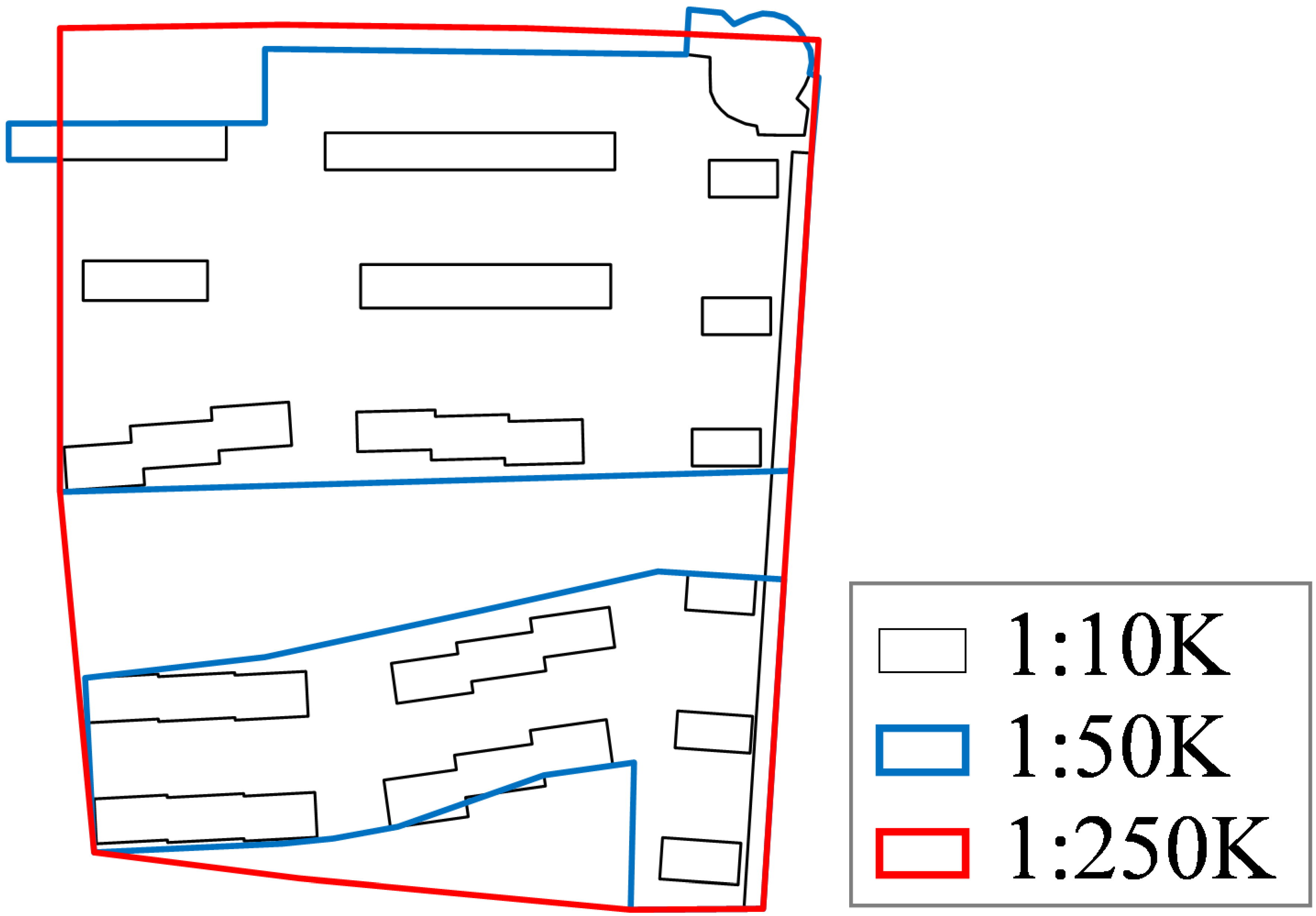
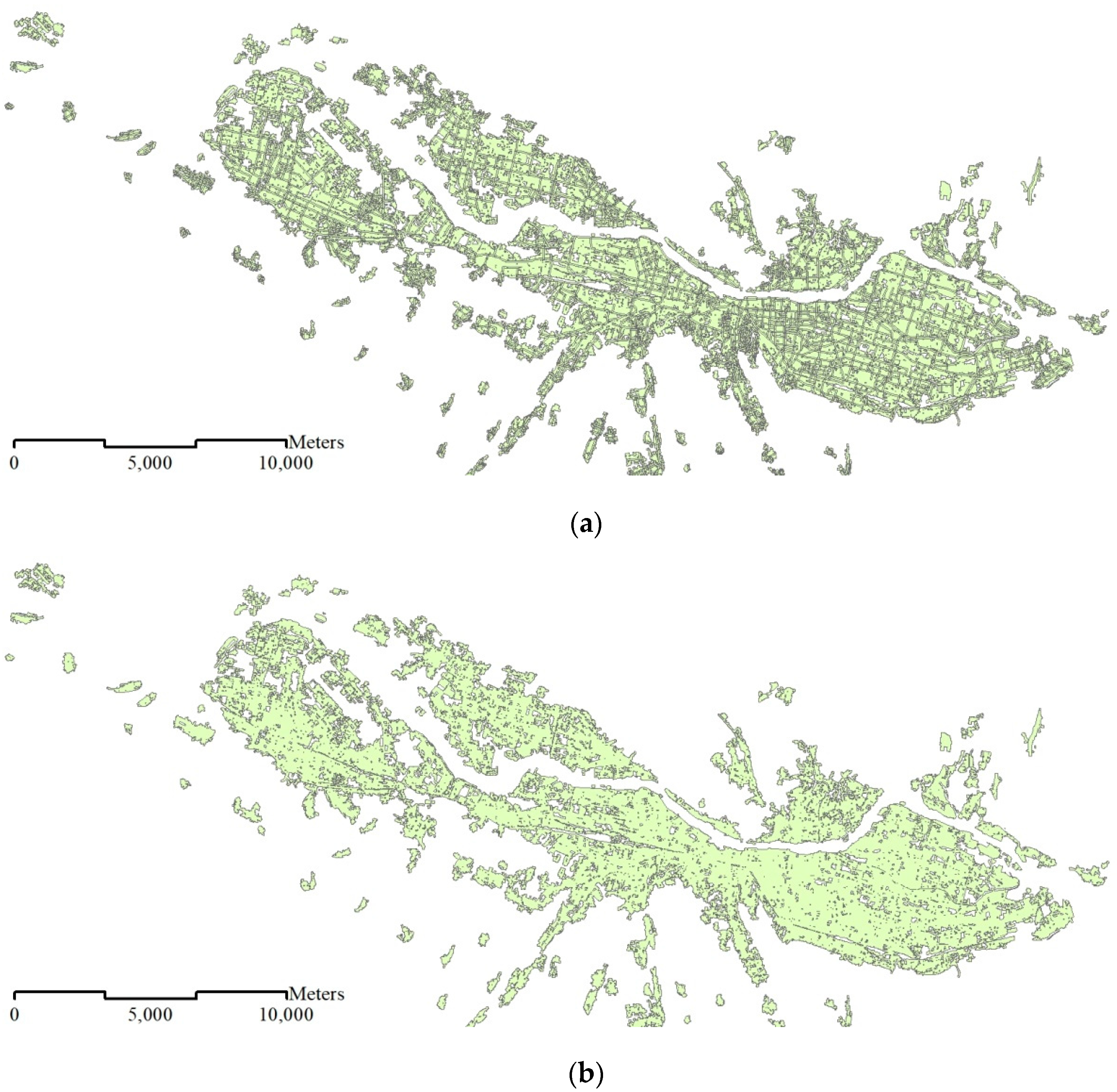
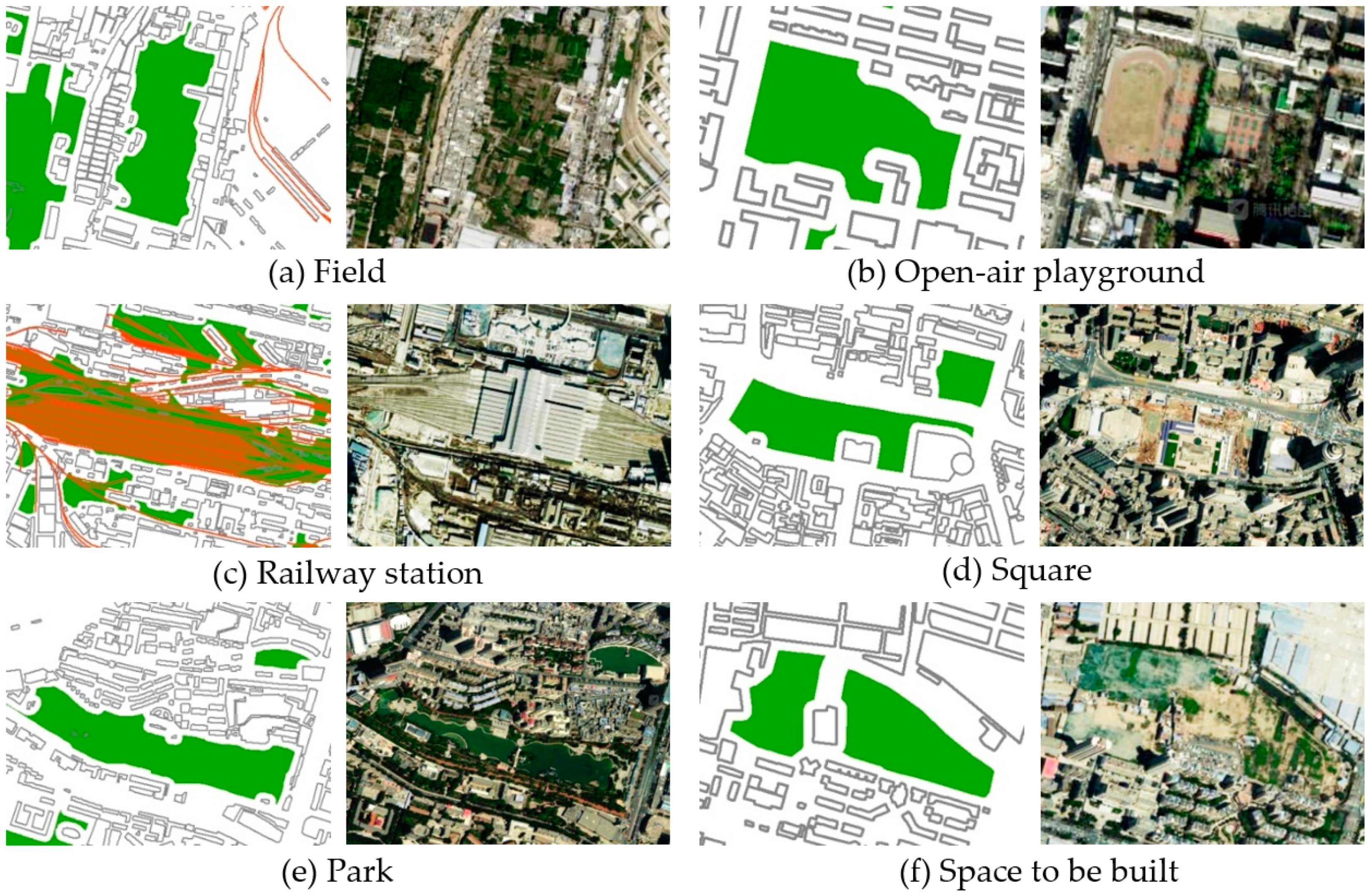
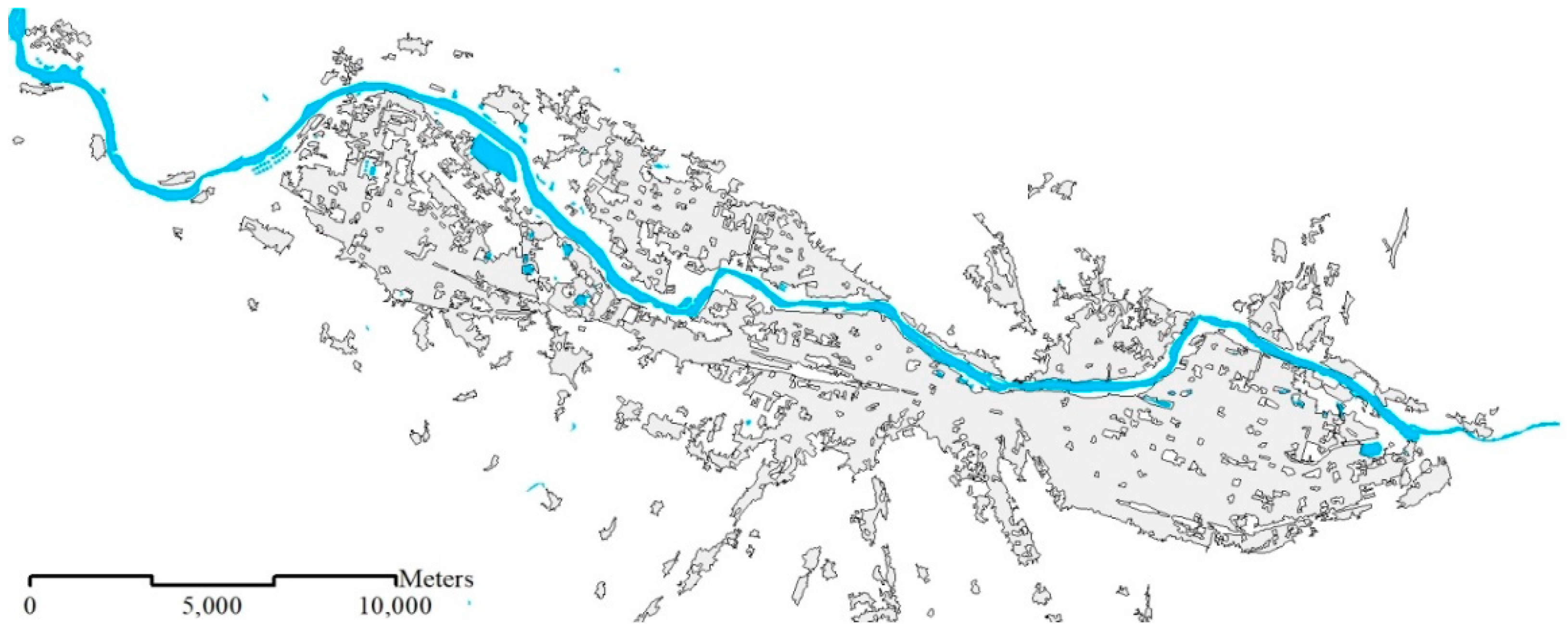
- In the 1:10K dataset, residential areas are represented as buildings (Figure 1a);
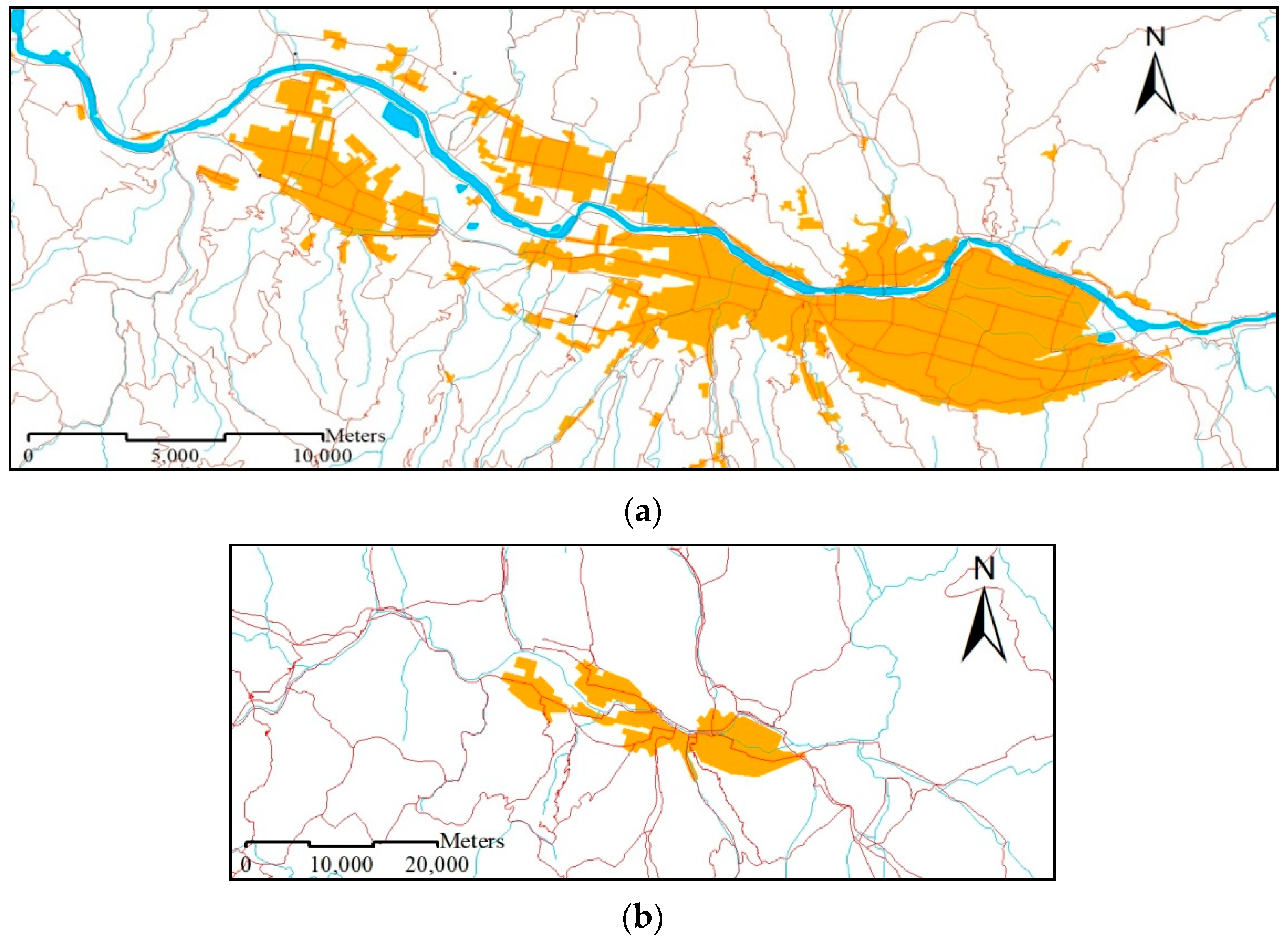
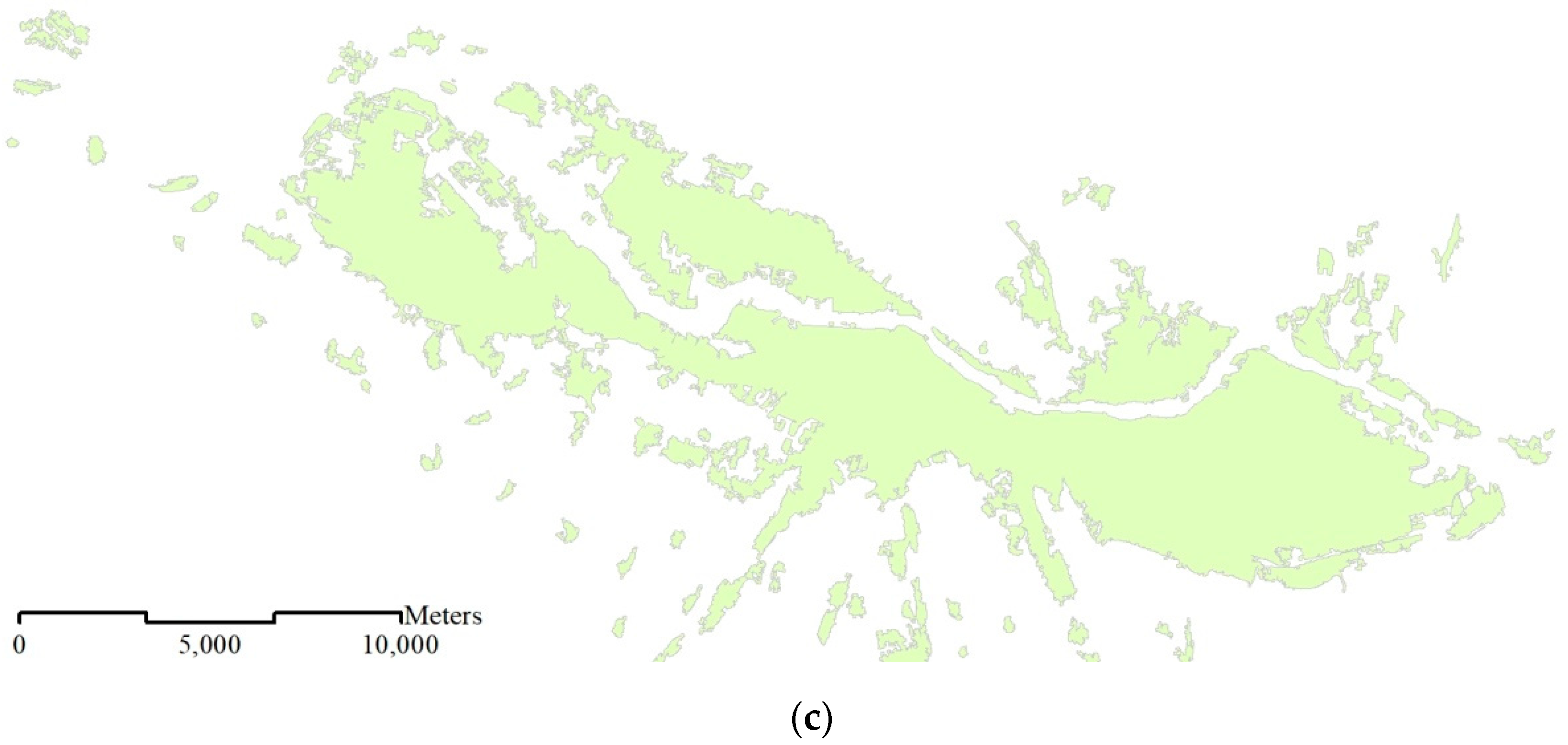
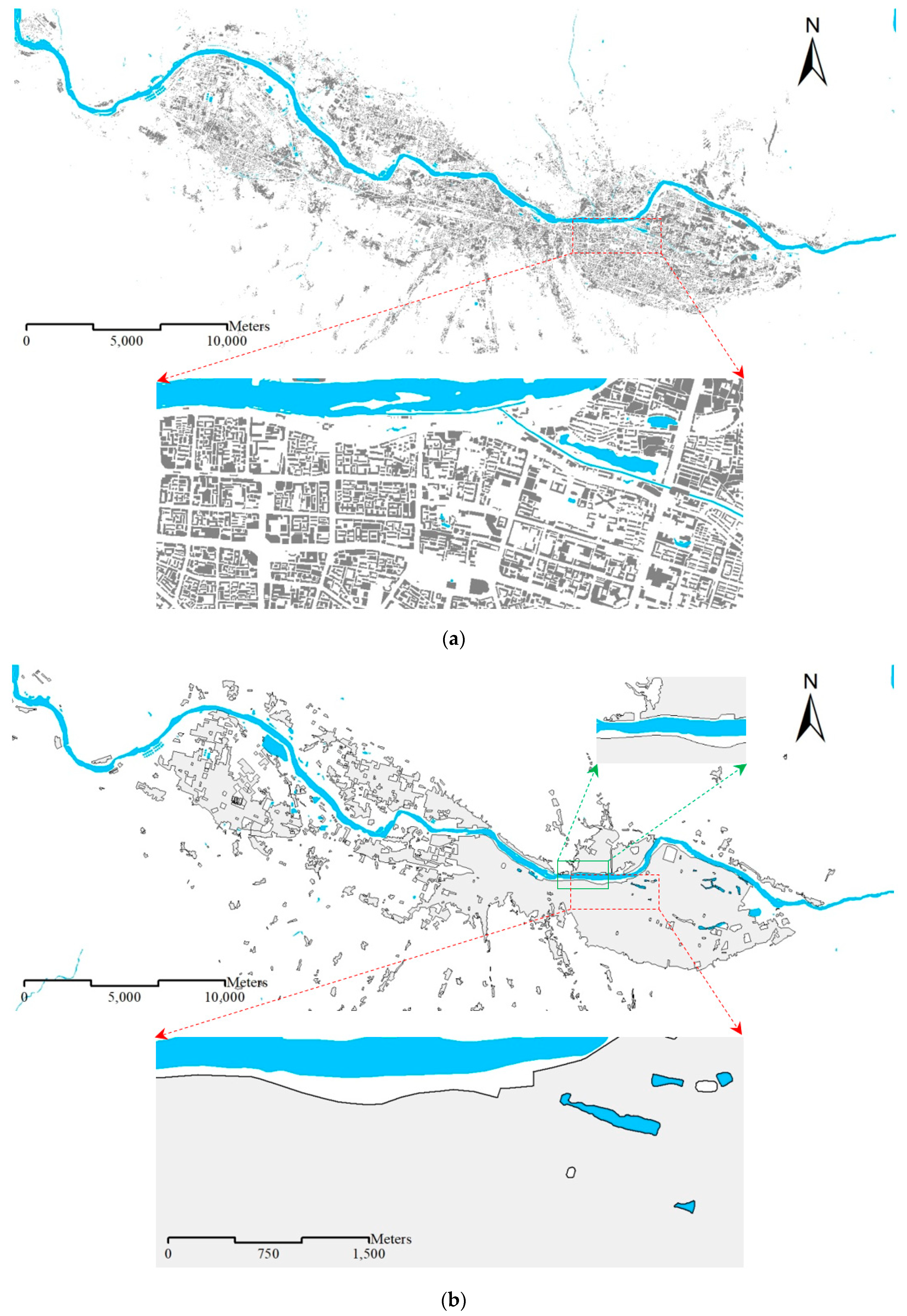
- In the 1:250K dataset, residential areas depict entire urban settlements (Figure 2a);
- In the 1:1M dataset, only big cities (i.e., residential areas) appear (Figure 2b).
2.2.2. Process Modeling
- Buffer Distance
- Selection Threshold
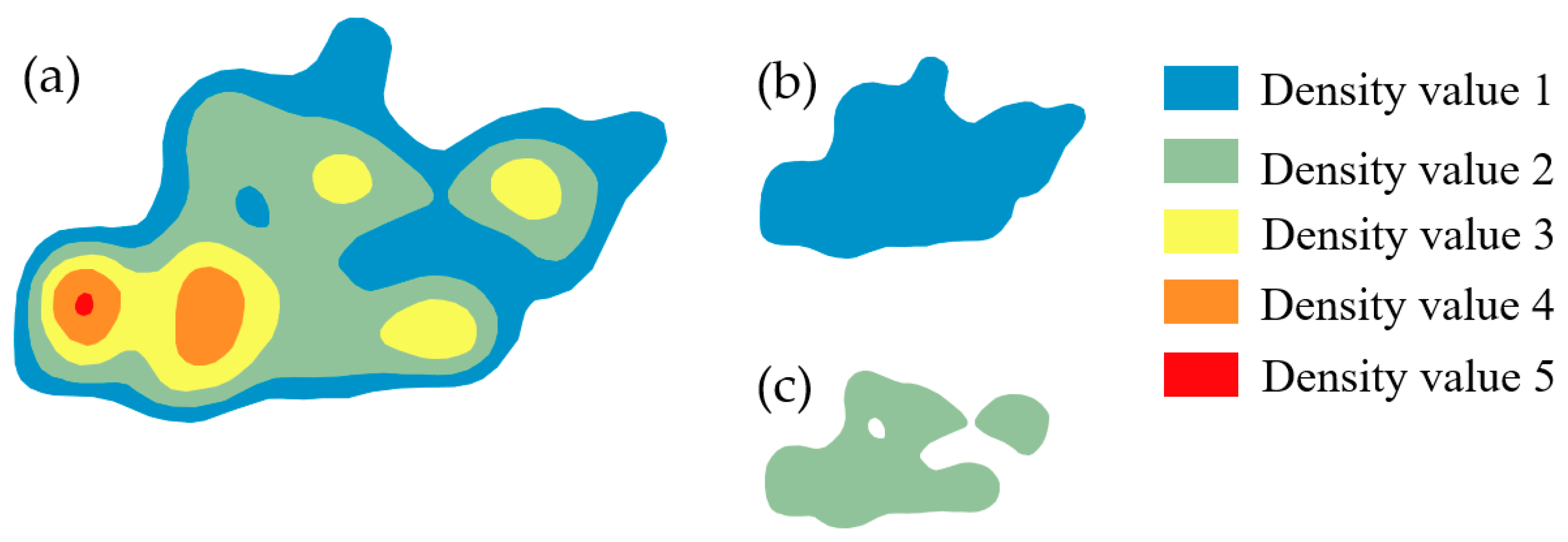
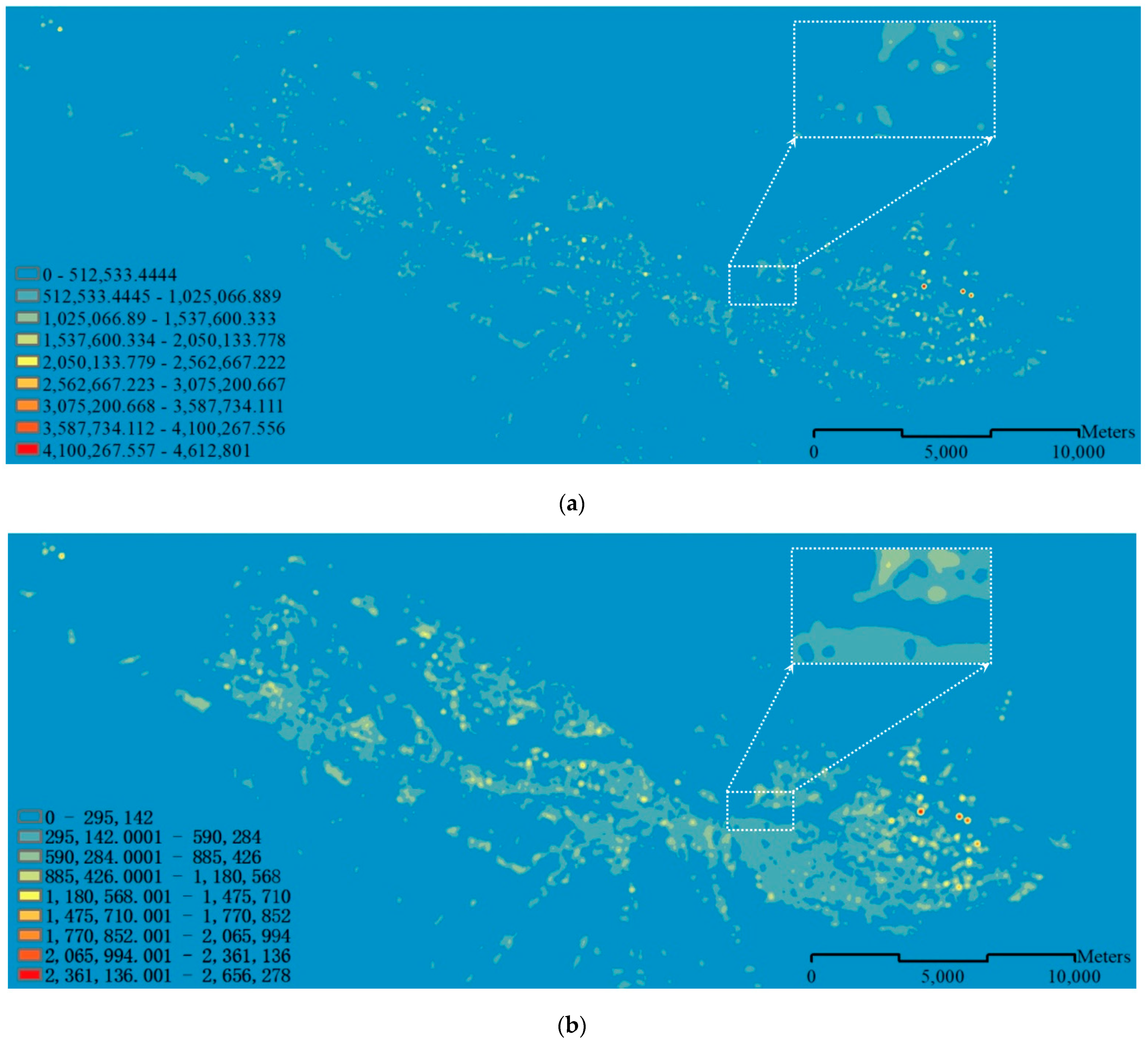
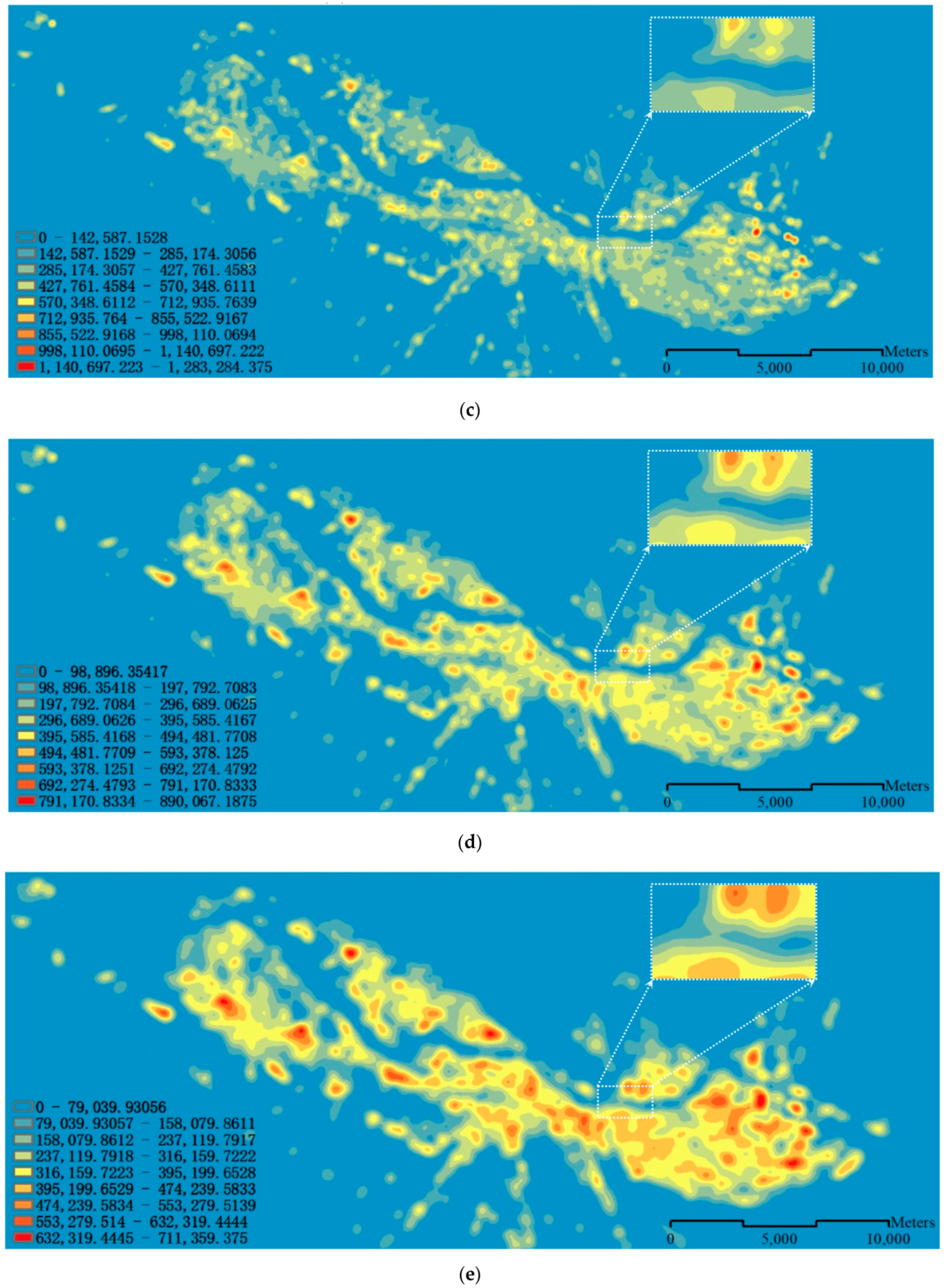
- KDE Threshold
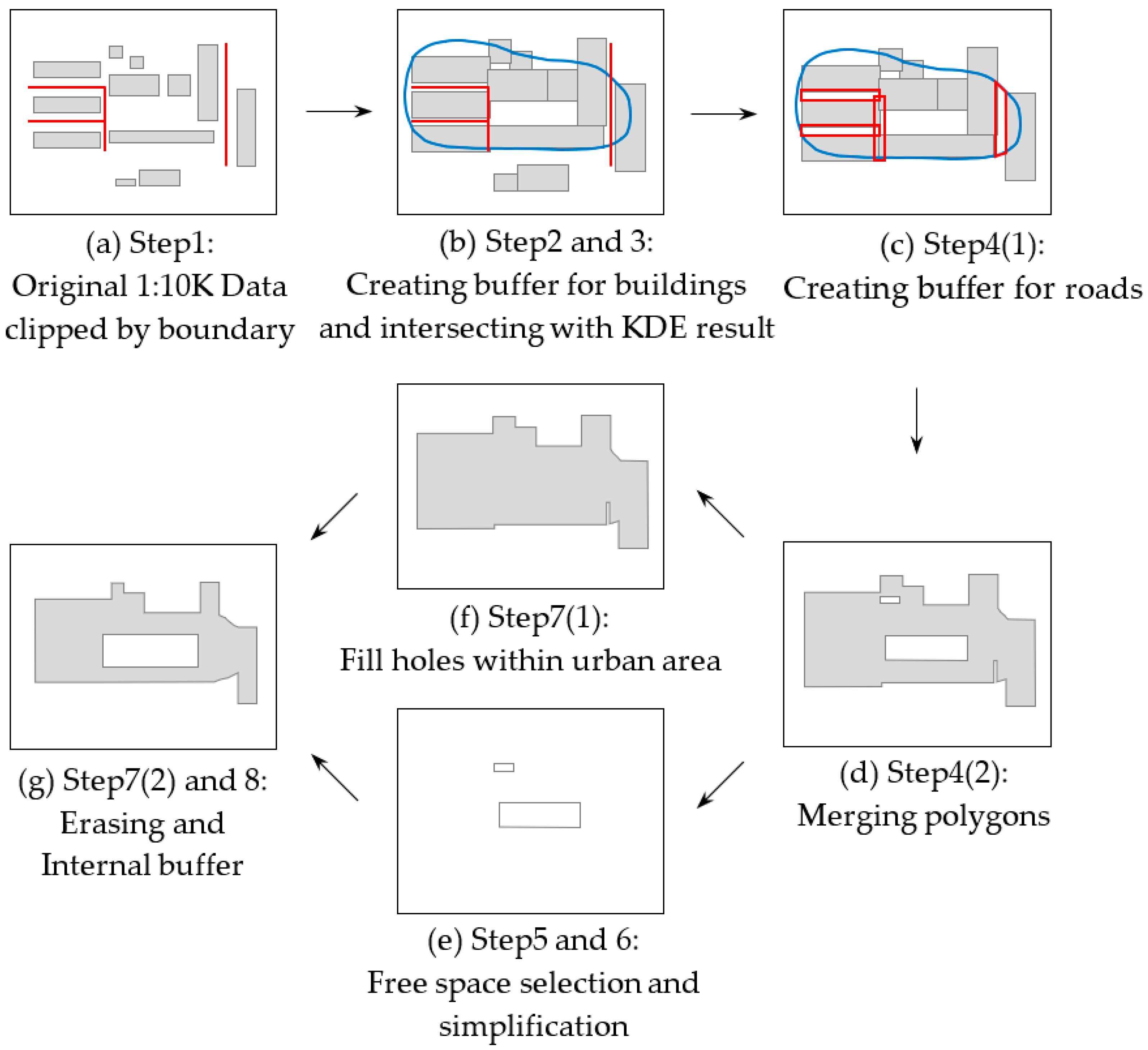
2.2.3. Detailed Generalization Process
3. Experiments and Results
3.1. Results and Analysis
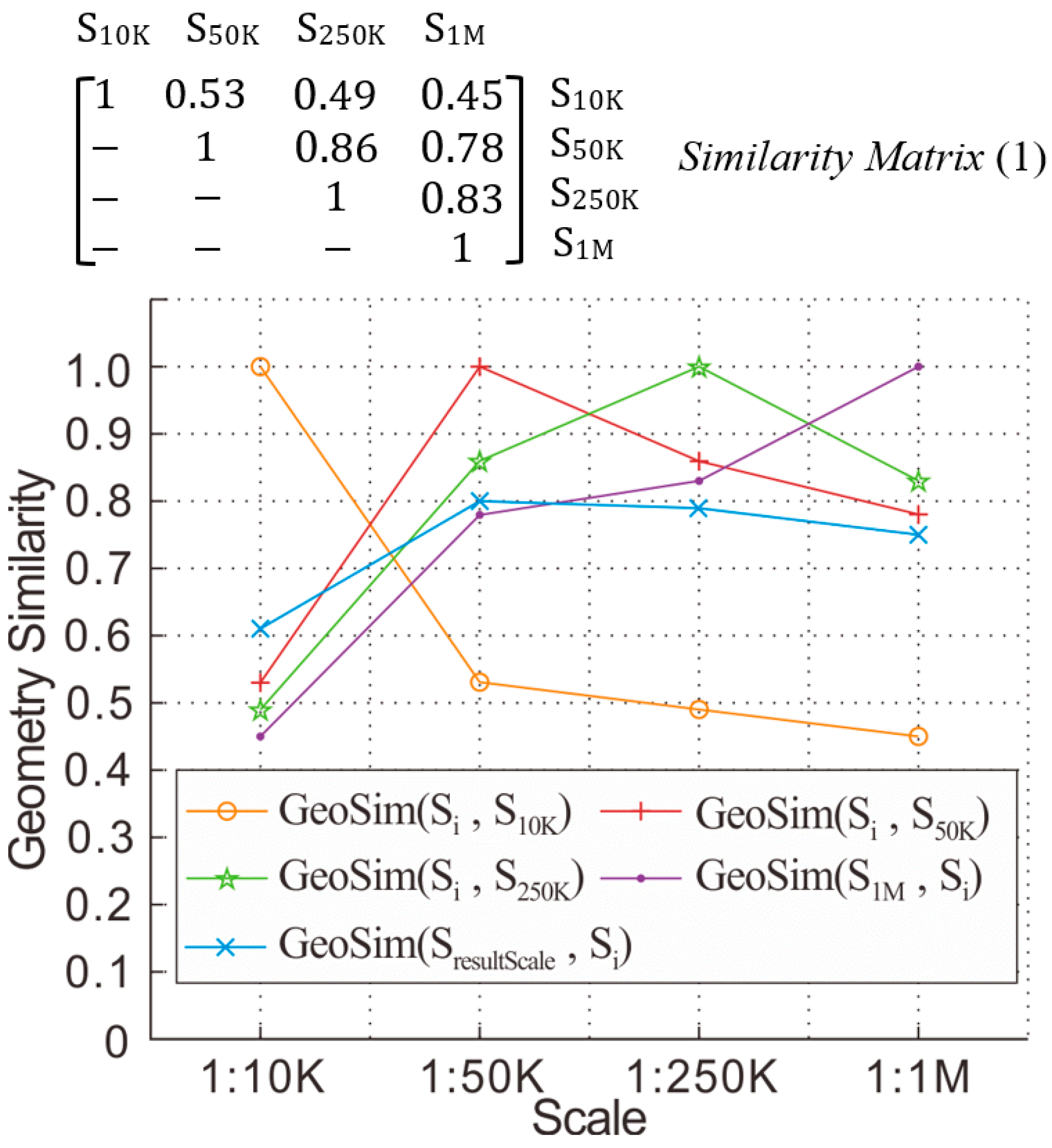
3.1.1. Geometric Similarity Results and Analysis
3.1.2. The KDE Results with Different Threshold Values and Manual Inspection
3.1.3. Similarity Measure and Threshold Determination
3.1.4. Results of Generalization
3.2. Evaluation
3.2.1. Visual Comparison with Reference 1:50K Data
3.2.2. Quantitative Evaluation
3.2.3. Satisfaction of Requirements in Practice
4. Discussion
5. Conclusions and Future Work
Author Contributions
Funding
Data Availability Statement
Conflicts of Interest
References
- Ruas, A. Automating the generalisation of geographical data: The age of maturity? In Proceedings of the 20th International Cartographic Conference, Beijing, China, 6 August 2001. [Google Scholar]
- Lee, D.; Hardy, P. Automating Generalization—Tools and Models. In Proceedings of the XXII International Cartographic Conference, La Coruna, Spain, 11–16 July 2005. [Google Scholar]
- Duchêne, C.; Ruas, A.; Cambier, C. The CartACom model: Transforming cartographic features into communicating agents for cartographic generalization. Int. J. Geogr. Inf. Sci. 2012, 26, 1533–1562. [Google Scholar] [CrossRef]
- Yang, M.; Ai, T.; Yan, X.; Chen, Y.; Zhang, X. A map-algebra-based method for automatic change detection and spatial data updating across multiple scales. Trans. GIS 2018, 22, 435–454. [Google Scholar] [CrossRef]
- Yu, W.; Zhang, Y.; Chen, Z. Automated generalization of facility points-of-interest with service area delimitation. IEEE Access 2019, 7, 63921–63935. [Google Scholar] [CrossRef]
- Yan, H.; Li, J. Spatial Similarity Relations in Multi-Scale Map Spaces; Springer International Publishing: Cham, Switzerland, 2015. [Google Scholar]
- Weibel, R.; Keller, S.; Reichenbacher, T. Overcoming the knowledge acquisition bottleneck in map generalization: The role of interactive systems and computational intelligence. In Proceedings of the 2nd International Conference on Spatial Information Theory (COSIT 95), Semmering, Austria, 21 September 1995. [Google Scholar]
- Kilpeläinen, T. Knowledge Acquisition for Generalization Rules. Cartogr. Geogr. Inf. Sci. 2000, 27, 41–50. [Google Scholar] [CrossRef]
- Mustiere, S. Cartographic generalization of roads in a local and adaptive approach: A knowledge acquistion problem. Int. J. Geogr. Inf. Sci. 2005, 19, 937–955. [Google Scholar] [CrossRef]
- Douglas, D.H.; Peucker, T.K. Algorithms for the reduction of the number of points required to represent a digitized line or its caricature. Can. Cartogr. J. 1973, 10, 112–122. [Google Scholar] [CrossRef] [Green Version]
- Regnauld, N.; Edwardes, A.; Barrault, M. Strategies in building generalization: Modelling the sequence, constraining the choice. In Proceedings of the 19th ICC Workshop on Progress and Developments in Automated Map Generalization, Ottawa, ON, Canada, 14–21 August 1999. [Google Scholar]
- Sester, M. Optimizing approaches for generalization and data abstraction. Int. J. Geogr. Inf. Sci. 2005, 19, 871–897. [Google Scholar] [CrossRef]
- Bayer, T. Automated building simplification using a recursive approach. In Cartography in Central and Eastern Europe; Gartner, G., Ortag, F., Eds.; Springer: Berlin/Heidelberg, Germany, 2009; pp. 121–146. [Google Scholar]
- Yan, X.; Ai, T.; Zhang, X. Template matching and simplification method for building features based on shape cognition. Int. J. Geo-Inf. 2017, 6, 250. [Google Scholar] [CrossRef] [Green Version]
- Yang, M.; Yuan, T.; Yan, X.; Ai, T.; Jiang, C. A hybrid approach to building simplification with an evaluator from a backpropagation neural network. Int. J. Geogr. Inf. Sci. 2021, 5, 1–30. [Google Scholar] [CrossRef]
- Su, B.; Li, Z.; Lodwick, G. Jean-Claude Muller Algebraic models for the aggregation of area features based upon morphological operators. Int. J. Geogr. Inf. Sci. 1997, 11, 233–246. [Google Scholar] [CrossRef]
- Li, Z.; Yan, H.; Ai, T.; Chen, J. Automated building generalization based on urban morphology and Gestalt theory. Int. J. Geogr. Inf. Sci. 2004, 18, 513–534. [Google Scholar] [CrossRef]
- QI, H.; Li, Z. An Approach to Building Grouping Based on Hierarchical Constraints. In the International Archives of the Photogrammetry, Remote Sensing and Spatial Information Sciences. Vol. ⅩⅩⅩⅤⅠⅠ. Part B2 (pp. 449–454). Available online: http://www.isprs.org/proceedings/XXXVII/congress/2_pdf/3_WG-II-3/13.pdf (accessed on 10 October 2021).
- Bader, M. Energy Minimization Methods for Feature Displacement in Map Generalization. Ph.D. Thesis, Universität Zürich, Zürich, Switzerland, 2001. [Google Scholar]
- Ai, T.; Zhang, X.; Zhou, Q.; Yang, M. A vector field model to handle the displacement of multiple conflicts in building generalization. Int. J. Geogr. Inf. Sci. 2015, 29, 1310–1331. [Google Scholar] [CrossRef]
- Pilehforooshha, P.; Karimi, M.; Mansourian, A. A new model combining building block displacement and building block area reduction for resolving spatial conflicts. Trans. GIS 2021, 25, 1366–1395. [Google Scholar] [CrossRef]
- Brassel, K.; Weibel, R. A Review and Conceptual Framework of Automated Map Generalization. Int. J. Geogr. Inf. Syst. 1988, 2, 229–244. [Google Scholar] [CrossRef]
- Mcmaster, R.B.; Shea, K.S. Generalization in Digital Cartography; Association of American Geographers: Washington, DC, USA, 1992. [Google Scholar]
- Galanda, M. Automated Polygon Generalization in a Multi Agent System. Ph.D. Thesis, Universität Zürich, Zürich, Switzerland, 2003. [Google Scholar]
- Sarjakoski, L.T. Conceptual Models of Generalisation and Multiple Representation. In Generalisation of Geographic Information: Cartographic Modelling and Applications; Mackaness, W., Ruas, A., Sarjakoski, L.T., Eds.; Elsevier: Oxford, UK, 2007; pp. 11–36. [Google Scholar]
- O’Keefe, J.; Dostrovsky, J. The hippocampus as a spatial map: Preliminary evidence from unit activity in the freely-moving rat. Brain Res. 1971, 34, 171–175. [Google Scholar] [CrossRef]
- O’Keefe, J.; Nadel, L. The Hippocampus as a Cognitive Map; Clarendon: Oxford, UK, 1978. [Google Scholar]
- Hafting, T.; Fyhn, M.; Molden, S.; Moser, M.; Moser, E. Microstructure of a spatial map in the entorhinal cortex. Nature 2005, 436, 801–806. [Google Scholar] [CrossRef] [PubMed]
- Yan, X.; Ai, T.; Yang, M.; Tong, X.; Liu, Q. A graph deep learning approach for urban building grouping. Geocarto Int. 2020, 8, 1–24. [Google Scholar] [CrossRef]
- Li, Z.; Huang, P. Quantitative measures for spatial information of maps. Int. J. Geogr. Inf. Sci. 2002, 16, 699–709. [Google Scholar] [CrossRef]
- Mackaness, W.A.; Burghardt, D.; Duchêne, C. Map Generalization. In International Encyclopedia of Geography: People, the Earth, Environment and Technology; Richardson, D., Castree, N., Goodchild, M.F., Kobayashi, A., Liu, W., Marston, R.A., Eds.; John Wiley & Sons Ltd.: Hoboken, NJ, USA, 2017. [Google Scholar] [CrossRef]
- Boffet, A.; Serra, S.R. Identification of spatial structures within urban blocks for town characterization. In Proceedings of the 20th International Cartographic Conference, Beijing, China, 6 August 2001; pp. 1974–1983. [Google Scholar]
- Chaudhry, O.; Mackaness, W. Automatic identification of urban settlement boundaries for multiple representation databases. Comput. Environ. Urban Syst. 2008, 32, 95–109. [Google Scholar] [CrossRef]
- Liu, Y.; Martin, M.; Menno-Jan, K. Semantic Similarity Evaluation Model in Categorical Database Generalization. In Proceedings of the Symposium on Geospatial Theory, Processing and Applications, Ottawa, ON, Canada, 9–12 July 2002. [Google Scholar]
- Zhou, Q. Comparative Study of Approaches to Delineating Built-Up Areas Using Road Network Data. Trans. GIS 2015, 19, 848–876. [Google Scholar] [CrossRef]
- Li, Y.; Sun, Q.; Ji, X.; Xu, L.; Lu, C.; Zhao, Y. Defining the Boundaries of Urban Built-up Area Based on Taxi Trajectories: A Case Study of Beijing. J. Geovisualization Spat. Anal. 2020, 4, 8. [Google Scholar] [CrossRef]
- Burghardt, D.; Steiniger, S. Usage of principal component analysis in the process of automated generalisation. In Proceedings of the 22nd International Cartographic Conference, La Coruna, Spain, 9–16 July 2005; International Cartographic Association (ICA): La Coruna, Spain, 2005. [Google Scholar]
- Du, S.; Luo, L.; Cao, K.; Shu, M. Extracting building patterns with multilevel graph partition and building grouping. Isprs J. Photogramm. Remote Sens. 2016, 122, 81–96. [Google Scholar] [CrossRef]
- Chaudhry, O.; Mackaness, W. Visualisation of Settlements over Large Changes in Scale. In Proceedings of the 8th ICA Workshop on Generalisation and Multiple Representation, La Coruna, Spain, 9–16 July 2005. [Google Scholar]
- Jiang, B.; Liu, X. Scaling of geographic space from the perspective of city and field blocks and using volunteered geographic information. Int. J. Geogr. Inf. Sci. 2012, 26, 215–229. [Google Scholar] [CrossRef] [Green Version]
- Smith, B. On drawing lines on a map. In Spatial Information Theory, Proceedings of COSIT ’95 Berlin/Heidelberg/Vienna/New York/London/Tokyo, Vienna, Austria, 21–23 September 1995; Frank, A.U., Kuhn, W., Mark, D., Eds.; Springer: Berlin/Heidelberg, Germany, 1995; pp. 475–484. [Google Scholar]
- Silverman, B.W. Density Estimation for Statistics and Data Analysis; Chapman and Hall: New York, NY, USA, 1986. [Google Scholar]
- Thurstain-Goodwin, M.T.; Unwin, D. Defining and delineating the central areas of towns for statistical monitoring using continuous surface representations. Trans. GIS 2000, 4, 305–317. [Google Scholar] [CrossRef]
- Borruso, G. Network Density and the Delimitation of Urban Areas. Trans. GIS 2003, 7, 177–191. [Google Scholar] [CrossRef]
- Borruso, G. Network Density Estimation: A GIS Approach for Analysing Point Patterns in a Network Space. Trans. GIS 2010, 12, 377–402. [Google Scholar] [CrossRef]
- Jia, T.; Jiang, B. Measuring Urban Sprawl Based on Massive Street Nodes and the Novel Concept of Natural Cities. arXiv 2011, arXiv:1010.0541. WWW Document. Available online: https://arxiv.org/ftp/arxiv/papers/1010/1010.0541.pdf (accessed on 10 October 2021).
- Tversky, A. Features of similarity. Psychol. Rev. 1977, 84, 327–352. [Google Scholar] [CrossRef]
- Holt, A. Spatial Similarity and GIS: The Grouping of Spatial Kinds. In Proceedings of the 11th Annual Colloquium of the Spatial Information Research Centre, Dunedin, New Zealand, 13–15 December 1999. [Google Scholar]
- Popper, K.R. The Logic of Scientific Discovery; Hutchinson: London, UK, 1972; 480p. [Google Scholar]
- Ai, T.; Ke, S.; Yang, M.; Li, J. Envelope generation and simplification of polylines using Delaunay triangulation. Int. J. Geogr. Inf. Sci. 2017, 31, 297–319. [Google Scholar] [CrossRef]
- Arkin, E.M.; Chew, L.P.; Huttenlocher, D.P.; Kedem, K.; Mitchell, J.S.B. An Efficiently Computable Metric for Comparing Polygonal Shapes. IEEE Trans. Pattern Anal. Mach. Intell. 1991, 13, 209–216. [Google Scholar] [CrossRef] [Green Version]
- Samal, A.; Seth, S.; Cueto, K. A feature-based approach to conflation of geospatial source. Int. J. Geogr. Inf. Sci. 2004, 18, 459–489. [Google Scholar] [CrossRef]
- Frank, R.; Ester, M. A quantitative similarity measure for maps. In Progress in Spatial Data Handling; Riedl, A., Kainz, W., Elmes, G.A., Eds.; Springer: Berlin, Germany, 2006; pp. 435–450. [Google Scholar]
- Goodchild, M.F.; Hunter, G.J. A simple positional accuracy measure for linear features. Int. J. Geogr. Inf. Sci. 1997, 11, 299–306. [Google Scholar] [CrossRef]
- Winecoff, A.A.; Brasoveanu, F.; Casavant, B. Users in the loop: A psychologically-informed approach to similar item retrieval. In Proceedings of the 13th ACM Conference on Recommender Systems, Copenhagen, Denmark, 16–20 September 2019. [Google Scholar]
- Wang, Z.; Müller, J.-C. Line Generalization Based on Analysis of Shape Characteristics. Cartogr. Geogr. Inf. Syst. 1998, 25, 3–15. [Google Scholar] [CrossRef]
- Rodríguez, M.A. Assessing Semantic Similarity among Spatial Entity Classes. Ph.D. Thesis, University of Maine, Orono, ME, USA, 2000. [Google Scholar]


| Scale | Updating Time | Usage |
|---|---|---|
| 1:10K | 2017–2019 | a. Data to validate the similarity measure; b. Data to be aggregated to obtain the target data. |
| 1:50K | 2012–2014 | a. Data to validate the similarity measure; b. Standard data. |
| 1:250K | 2012 | a. Data to validate the similarity measure. |
| 1:1M | 2015 | a. Data to validate the similarity measure. |
| Object Data and Reference Data | Common Area (m2) | Symmetrical Difference Area (m2) | Similarity Value |
|---|---|---|---|
| 1:50K, 1:10K | 43,071,658 | 74,941,399 | 0.53 |
| 1:250K, 1:10K | 40,623,846 | 85,319,088 | 0.49 |
| 1:1M, 1:10K | 39,926,929 | 98,906,243 | 0.45 |
| 1:250K, 1:50K | 92,497,605 | 28,961,830 | 0.86 |
| 1:1M, 1:50K | 88,426,174 | 49,297,954 | 0.78 |
| 1:1M, 1:250K | 96,648,146 | 38,336,073 | 0.83 |
| Threshold (m) | Common Area (m2) | Symmetrical Difference Area (m2) | Similarity |
|---|---|---|---|
| 150 | 20,470,299 | 87,143,961 | 0.32 |
| 200 | 66,457,811 | 52,045,137 | 0.72 |
| 300 | 98,036,747 | 59,650,663 | 0.77 |
| 400 | 101,323,067 | 83,361,424 | 0.71 |
| 500 | 102,154,882 | 102,910,295 | 0.67 |
| 600 | 102,457,973 | 116,361,813 | 0.64 |
| Object Data (Resulting Data) and Reference Data | Common Area (m2) | Symmetrical Difference Area (m2) | Similarity |
|---|---|---|---|
| Result, 1:10K | 53,260,312 | 68,916,946 | 0.61 |
| Result, 1:50K | 88,326,204 | 44,336,786 | 0.80 |
| Result, 1:250K | 89,024,948 | 48,421,362 | 0.79 |
| Result, 1:1M | 89,229,289 | 60,206,001 | 0.75 |
| Criterion | Traditional Method | Proposed Method |
|---|---|---|
| 1:10K and 1:50K data updating mode | Manual updating | 1:10K data updating + 1:50K data generalization from the newest 1:10K data |
| Data updating cycle | Longer (1:10K data manual updating cycle + 1:50K data manual updating cycle) | Shorter (1:10K manual updating cycle + automatic 1:50K data generalization time) |
| Consistency between 1:10K data and 1:50K data | Not good before updating is finished | Good |
| Correctness of outer boundaries and free spaces | Depends on the cartographer’s experience and skill | Correctness can be ensured due to the dilating and eroding buffers of updated buildings and roads |
| Threshold determination automation | / | Yes |
| Method is objective or Subjective | Subjective | Objective |
Publisher’s Note: MDPI stays neutral with regard to jurisdictional claims in published maps and institutional affiliations. |
© 2022 by the authors. Licensee MDPI, Basel, Switzerland. This article is an open access article distributed under the terms and conditions of the Creative Commons Attribution (CC BY) license (https://creativecommons.org/licenses/by/4.0/).
Share and Cite
Gao, X.; Yan, H.; Lu, X.; Li, P. Automated Residential Area Generalization: Combination of Knowledge-Based Framework and Similarity Measurement. ISPRS Int. J. Geo-Inf. 2022, 11, 56. https://doi.org/10.3390/ijgi11010056
Gao X, Yan H, Lu X, Li P. Automated Residential Area Generalization: Combination of Knowledge-Based Framework and Similarity Measurement. ISPRS International Journal of Geo-Information. 2022; 11(1):56. https://doi.org/10.3390/ijgi11010056
Chicago/Turabian StyleGao, Xiaorong, Haowen Yan, Xiaomin Lu, and Pengbo Li. 2022. "Automated Residential Area Generalization: Combination of Knowledge-Based Framework and Similarity Measurement" ISPRS International Journal of Geo-Information 11, no. 1: 56. https://doi.org/10.3390/ijgi11010056
APA StyleGao, X., Yan, H., Lu, X., & Li, P. (2022). Automated Residential Area Generalization: Combination of Knowledge-Based Framework and Similarity Measurement. ISPRS International Journal of Geo-Information, 11(1), 56. https://doi.org/10.3390/ijgi11010056