Classification of Airborne Laser Scanning Point Cloud Using Point-Based Convolutional Neural Network

Abstract

In various applications of airborne laser scanning (ALS), the classification of the point cloud is a basic and key step. It requires assigning category labels to each point, such as ground, building or vegetation. Convolutional neural networks have achieved great success in image classification and semantic segmentation, but they cannot be directly applied to point cloud classification because of the disordered and unstructured characteristics of point clouds. In this paper, we design a novel convolution operator to extract local features directly from unstructured points. Based on this convolution operator, we define the convolution layer, construct a convolution neural network to learn multi-level features from the point cloud, and obtain the category label of each point in an end-to-end manner. The proposed method is evaluated on two ALS datasets: the International Society for Photogrammetry and Remote Sensing (ISPRS) Vaihingen 3D Labeling benchmark and the 2019 IEEE Geoscience and Remote Sensing Society (GRSS) Data Fusion Contest (DFC) 3D dataset. The results show that our method achieves state-of-the-art performance for ALS point cloud classification, especially for the larger dataset DFC: we get an overall accuracy of 97.74% and a mean intersection over union (mIoU) of 0.9202, ranking in first place on the contest website.

1. Introduction

The three-dimensional (3D) point cloud has become an important data source for reconstructing and understanding the real world because of its abundant geometry, shape and scale information. Among the many methods for obtaining 3D point clouds, airborne laser scanning (ALS) or light detection and ranging (LiDAR) are important technologies for obtaining high-precision and dense point clouds of large-scale ground scenes. Many applications of ALS point clouds have been explored, such as digital elevation model (DEM) generation [1,2], building reconstruction [3,4], road extraction [5,6], forest mapping [7,8], power line monitoring [9,10] and so on. For these applications, the basic and critical step is the classification of the 3D point cloud, which is also called semantic segmentation of the point cloud in the field of computer vision. It requires the assignment of semantic labels, such as ground, building and vegetation, to each point. Point cloud classification is very important for understanding scenes and the subsequent processing of point clouds. However, due to the unstructured and disordered characteristics of point clouds, especially in urban scenes with different object types and variable point densities, the accurate and efficient classification of ALS point clouds is still a challenging task.

Early research on ALS point cloud classification focused on extracting handcrafted features, such as eigenvalues [11,12], shape and geometry features [13,14,15] and using traditional supervised classifiers, such as support vector machine (SVM) [16,17,18], random forests [19,20], AdaBoost [14,21], Markov random field (MRF) [22,23,24], conditional random field (CRF) [25,26] and so on. However, these traditional machine learning-based methods rely heavily on professional experience and have limited generalizability when applied to complex, large-scale scenes [27]. In recent years, deep learning methods, especially the convolutional neural network (CNN), have achieved great success in two-dimensional (2D) image classification [28,29,30] and semantic segmentation [31,32,33] due to the implicit ability to learn high-dimensional features. Inspired by this major breakthrough, researchers have begun to use deep learning-based methods for 3D point classification. However, due to the unordered and unstructured characteristics of point clouds, CNN for image semantic segmentation cannot be applied directly to point cloud classification. Some works transform an irregular 3D point cloud into regular 2D images or 3D voxels, which can be classified by 2D CNN or 3D CNN [34,35,36,37]. However, this transformation leads to the loss of information. Some recent methods have tried to build a point-based CNN to classify irregular point clouds directly [27,38,39,40,41,42,43,44]. However, these methods are inefficient for learning multi-level point features. Some methods still need to input some low-level geometric features to improve the classification accuracy.

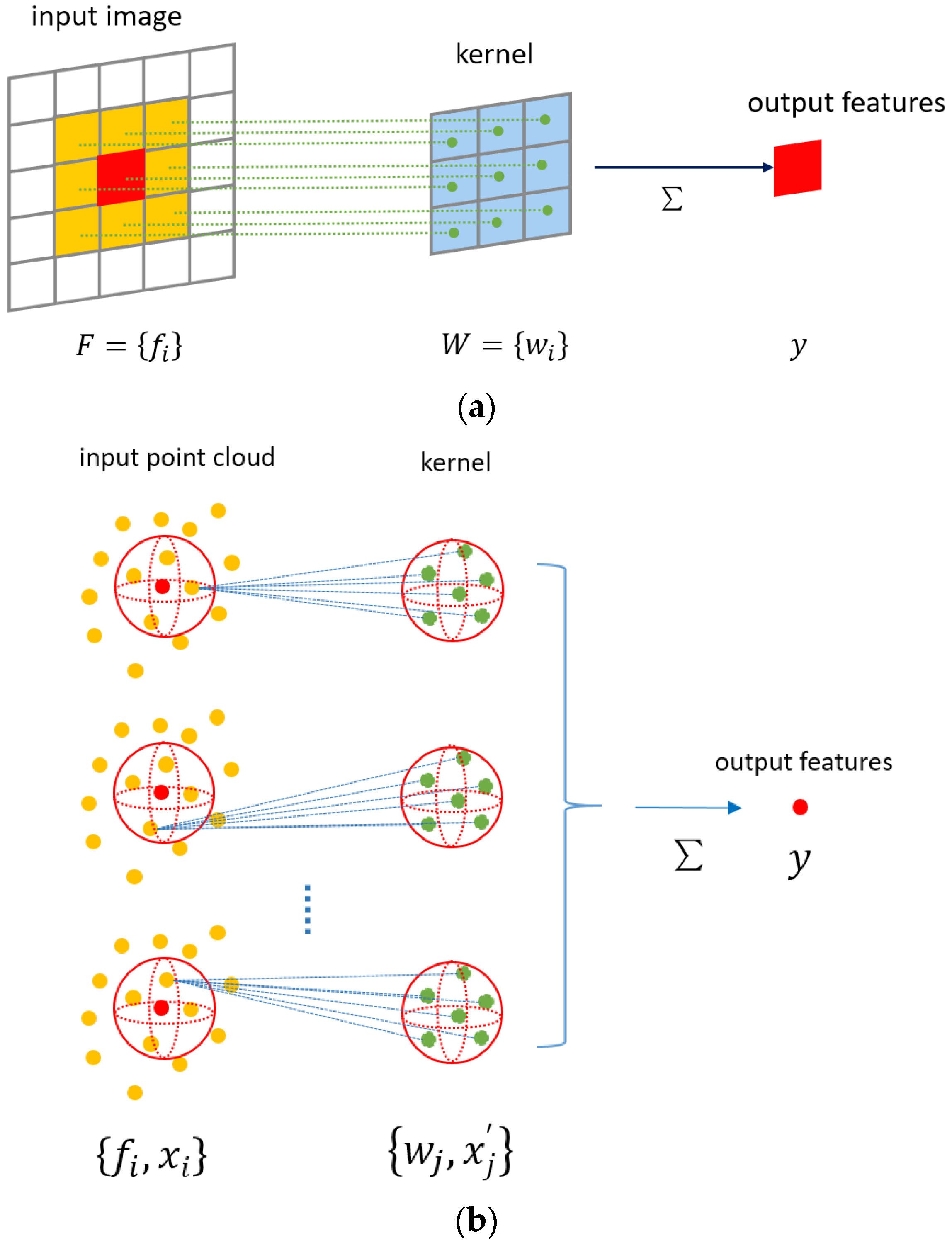
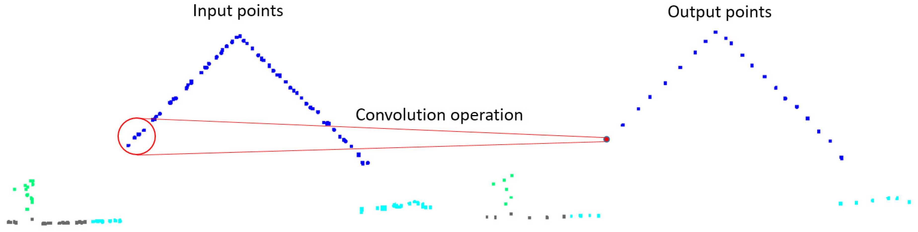
In this paper, we propose a novel, point-based CNN to classify ALS data. The method can directly take the raw 3D point cloud as an input. The local point features are learned efficiently by a convolution operation designed for unstructured points. Then, we build a classification network by stacking with multi-convolution layers, which is constructed based on the convolution operation. The network has the structure of encoder and decoder, which is similar to U-net, flexible and easy to expand. Multi-scale features are learned through a classification network and class labels are predicted for each point in an end-to-end fashion.

The main contributions of our method are summarized as follows.

(1)

A new convolution operator is designed, which can directly learn local features from an irregular point cloud without transforming to images or voxels. This is more adaptable and efficient than the handcrafted features.

(2)

A multi-scale CNN with an encoder and decoder structure is proposed. It can learn multi-level features directly from the point cloud and classify the ALS data in an end-to-end manner. The network is flexible and extensible.

(3)

The proposed method demonstrates state-of-the-art performance on two ALS datasets: the ISPRS Vaihingen 3D labeling benchmark and the 2019 IEEE GRSS Data Fusion Contest dataset.

The remainder of this paper is organized as follows. In Section 2, we briefly review the methods of ALS point cloud classification. Section 3 gives a detailed introduction to the proposed method. In Section 4, the performance of our method is evaluated, using two ALS datasets. We compare our results with other methods in Section 5. Finally, Section 6 presents some concluding remarks.

2. Related Work

Existing methods for ALS point cloud classification can generally be grouped into two main categories: traditional machine learning-based methods and deep learning-based methods. This is reviewed in the following.

2.1. Traditional Machine Learning-Based Methods

Early studies focused on extracting handcrafted features and using the traditional supervised classifier to classify ALS point clouds. Lodha et al. [16,21,45] resampled an irregular ALS point cloud onto a regular grid and registered it with gray-scale aerial imagery. Then, five features (height, height variation, normal variation, LiDAR return intensity and image intensity) and the SVM, AdaBoost and the expectation–maximization (EM) algorithm were used to classify airborne LiDAR data. In [17,19,46], the feature relevance of airborne LiDAR (multi-echo and full waveform) and multispectral image data were studied, and the SVM and random forest algorithm were chosen as a classifier. Guo et al. [13] computed 26 features from the LiDAR data based on geometry, intensity and multi-return information, using the JointBoost classifier. Weinmann et al. [12] made a systematic summary of the methods at this stage and presented a framework for 3D point cloud classification. This framework was composed of four parts: neighborhood selection, feature extraction, feature selection and classification. Seven neighborhood definitions, 21 geometric features, seven approaches for feature selection and 10 classifiers were studied.

The above methods classify each point independently, ignoring the context information between the neighboring points. This will result in classification noise and an inconsistent label. To address this problem, some works incorporated contextual information into the point cloud classification. Gerke et al. [22] performed the voxelization and segmentation of the point cloud, and then random trees and MRF were pursued in the classification. Niemeyer et al. [25] integrated random forest into a CRF framework to address the contextual classification task of airborne LiDAR point clouds. Zhu et al. [23] proposed a supervoxel-based method. Multi-level semantic constraints, including point-homogeneity, supervoxel-adjacency and class-knowledge constraints, were modeled in a MRF framework. Vosselman et al. [26] proposed a contextual, segment-based classification, using a CRF. The above methods commonly used the MRF or CRF framework to combine contextual information. However, they still need to extract handcrafted features, and it is difficult to apply these methods to the classification of point clouds in large scenes.

2.2. Deep Learning-Based Methods

Compared with the traditional machine learning-based methods, deep learning approaches do not rely on expensive handcrafted features. As an important deep learning technique, the CNN has achieved great success in 2D image classification. However, due to the unordered and unstructured characteristic of point clouds, the CNN cannot be applied directly to point cloud classification. Some researchers tried to transform point clouds into regular 2D images and then use 2D CNN to classify them. For example, Yang et al. [34] transferred the classification of a point to the classification of its corresponding feature image. First, the features of each point were extracted and transformed into an image. Then, a deep CNN model was trained with the feature images of the labeled points. Finally, the trained model was used to classify the unlabeled point cloud. Zhao et al. [35] first created a set of multi-scale contextual images for each point. Then, a designed multi-scale CNN was applied to automatically learn deep features for each point from its contextual images. Finally, the label of the point was outputted by using a softmax classifier with the learned deep features. However, the transformation from a 3D point cloud to 2D image will lead to a loss of information. Some other works voxelized the point clouds as regular 3D grids, and then applied a 3D CNN. For example, Huang et al. [36] proposed a voxel-based, 3D CNN for point cloud labeling. The raw point cloud was parsed through a voxelization process that generates occupancy voxel grids. Then, the occupied voxels and labels were fed to a 3D CNN to resolve the optimal parameters during training. In the testing module, the voxels generated by the point cloud without labels were passed to the trained 3D CNN to obtain the inferred labels. Although this method takes advantage of a 3D CNN through the voxelization of point clouds, it requires too much memory from the computer and too much time for computation.

In recent years, some point-based convolution neural networks have been proposed in the field of computer vision, which can directly deal with irregular point clouds. As a pioneering work, Qi et al. [47] proposed a deep learning framework named PointNet, which learned features directly from the raw point cloud. PointNet learned per-point features with several shared multi-layer perception (MLP) layers and extracted global shape features with a max-pooling layer. To capture the wider context for each point and learn the richer local structures, Qi et al. [48] further designed a hierarchical neural network called PointNet++, which applies PointNet recursively on a nested partitioning of the input point set. PointNet++ is mainly composed of a set abstract module and a feature propagation module for point feature downsampling and upsampling, respectively. Inspired by PointNet and PointNet++, many point-based networks have been proposed recently. In PointCNN [49], an χ-transform was learned and applied to a point cloud to achieve permutation invariance. Then, the typical convolution operator was applied to the χ-transform features. Jiang et al. [50] designed a module named PointSIFT, which can encode information of different directions and adapt to the scale of shapes. The module can be integrated into PointNet++ to improve its representation ability. Because the shared MLP layers are not sufficiently effective at learning point features, some works designed more effective convolution operations for point clouds to extract the point-wise features. Thomas et al. [51] proposed Kernel Point Convolution (KPConv), which operates on point clouds without any intermediate representation. The convolution weights of KPConv are located in the Euclidean space by kernel points and applied to the neighboring points. Boulch [52] proposed continuous convolutions (ConvPoint) for point cloud processing to replace the discrete kernels. It can be easily applied to the design of neural networks, just like 2D CNN. Other methods include PointConv [53], RandLA-Net [54], etc. Recently, Guo et al. [55] reviewed these methods in detail.

The above-mentioned point-based CNN methods have achieved impressive performance in the classification of point cloud in various indoor scenes, such as S3DIS [56] and ScanNet [57]. However, these methods cannot directly be applied to the large-scale ALS data because there are significant differences between the airborne LiDAR point cloud and indoor point cloud in sensor orientation, occlusion, data volume, object types and density. Some works modified these networks to classify airborne LiDAR point clouds. Wang et al. [38] proposed a deep neural network with spatial pooling (DNNSP), which uses a similar structure to PointNet to learn point cluster-based features. However, the point features are not learned directly from the point cloud, but by inputting the traditional point feature descriptors, such as spin images and eigenvalue features. Strictly speaking, it is not an end-to-end learning process. Yousefhussien et al. [39] presented a PointNet-based 1D fully convolutional network, which takes the terrain-normalized points and the corresponding spectral data as inputs. However, the normalized elevation values of the points are obtained by subtracting the DEM generated by the ground point, but these ground points cannot be obtained before the completion of classification. This decreases the adaptability of this method. Soilán et al. [42] used a classification model based on PointNet and compared heuristic and deep learning-based methods for ground classification from aerial point clouds. Winiwarter et al. [40] investigated the applicability of PointNet++ for the classification of airborne LiDAR data. alsNet was designed based on PointNet++, which deals with massive point clouds by introducing a batch processing framework. Arief et al. [41] proposed a method called Atrous XCRF to address the overfitting and poor generalization issues when training with a limited number of labeled points. The method works by forcing a trained model to respect the similarity penalties provided by unlabeled data. Wen et al. [27] designed a directionally constrained point convolution (D-Conv) module to extract locally representative features of point clouds. A directionally constrained, fully CNN (D-FCN) was applied to classify unstructured 3D point clouds. However, these methods are not efficient in learning multi-level features of points. Some methods still need to input some low-level geometric features to improve classification accuracy. This research is dedicated to the development of an efficient convolution operation for point clouds and a flexible and extensible CNN to learn multiscale point features and classify airborne LiDAR point clouds in an end-to-end fashion.

3. Methodology

In the task of point cloud classification, it is very important to extract the local and global features of points. As we know, the local features extraction of image is realized by a convolution kernel. However, due to the irregular distribution of the point cloud, the existing image convolution operator cannot be used directly. It is necessary to design a new convolution operator for point clouds. In Section 3.1, the convolution operator for point clouds is presented. Then, the convolution layer, constructed with the newly designed convolution operator, is presented in Section 3.2. Finally, in Section 3.3, using the convolution layer, we build a multi-scale CNN for point cloud classification.

3.1. Convolution Operator for Point Cloud

In image CNN, the feature aggregation of pixels is realized by a convolution operation. The convolution operation of image pixels is shown in Figure 1a. Firstly, the neighboring pixels in a small neighborhood area around the target pixel are obtained, such as the 3 × 3 area around the target pixel in Figure 1a. Then a convolution kernel of the same size is defined, and the features of the neighboring pixels are weighted by the convolution kernel elements. At last, the new feature of the target pixel is obtained by summing up the weighted features of neighboring pixels to realize local feature aggregation. Since the input features and kernels are ordered and they have the same size, the convolution operation can be defined as follows:

$$y={\displaystyle \sum }_{i=1}^N{w}_i{f}_i$$

(1)

where $f_i$ is the element features $F=\left\{f_i\right\}$ of neighboring pixels, and $i\in \left[1, N\right]$, $N$ is the number of neighboring pixels. These features can be the RGB color of the image pixel. $w_i$ is the element of the kernel weight $W=\left\{w_i\right\}, i\in \left[1, N\right]$.

Figure 1. A brief description of the comparison between image convolution and point cloud convolution. (a) Image convolution: Each pixel of the input image corresponds to one kernel element. (b) Point cloud convolution: Each point within the local region is weighted to all kernel elements.

Inspired by image convolution, for the feature aggregation of the point cloud, a neighborhood centered on the target point $p$ is defined first. Because the point cloud is in three-dimensional space, the neighborhood is generally set to be spherical. By giving a spherical radius or setting the number of nearest points, all the neighboring points in the neighborhood can be found, as shown in Figure 1b. Then a spherical convolution kernel is designed for the spherical neighborhood of the target point. Because the distribution of neighboring points is irregular instead of on a fixed grid, the positions of convolution kernel elements can also be irregularly distributed. Here, the convolution kernel elements are randomly located in one unit sphere, as the green points shown in Figure 1b. The number of convolution kernel elements is input as a parameter, which can be freely set as required, and it does not need to be the same as the number of neighbors. When defining the convolution kernel, the weights and positions of convolution kernel elements are randomly selected, and they are updated by the back propagation algorithm during the training.

Because there is no one-to-one correspondence between neighboring points and convolution kernel elements, the convolution of the point cloud cannot directly multiply the features of the neighboring points with the weights of corresponding convolution kernel elements, such as image convolution with the added weighted features to complete feature aggregation. When defining the convolution operation for a point cloud, it is necessary to consider the spatial relationship between the neighboring points and convolution kernel elements. Firstly, through a transformation function $T$, the new features of neighboring points are calculated from original features $f_i$ and the spatial relationship between neighboring points and convolution kernel elements. Then, function $A$ is used to aggregate all the transformed neighbor features to obtain the output feature of target point $p$. The convolution operation for point clouds can be defined as follows:

$$y=A \left( \left\{ T \left( f_i \right) | i\in N\left(p\right) \right\} \right)$$

(2)

where $N\left(p\right)$ represents the neighborhood of the target point $p$. $f_i$ is the element of features $F=\left\{f_i\right\}$ of input neighboring points. The features can be the intensity, return number, RGB color or other features of the point. As for function $T$, when we calculate the new feature of each neighboring point, we need to consider the positional relationship between the neighboring point and each convolution kernel element, so it is defined as follows:

$$T\left( f_i \right)={\displaystyle \sum }_{j=1}^M\phi \left(x_i, x_j^{\prime }\right)w_j{f}_i$$

(3)

where $w_j$ is the element of the kernel weight $W=\left\{w_j\right\}, j\in \left[1, M\right]$. $M$ is the number of kernel elements. Function $\phi \left(x_i, x_j^{\prime }\right)$ represents the spatial relationship between the input neighboring points and kernel elements, where $x_i$ and $x_j^{\prime }$ are the positions of neighboring point $i$ and kernel element $j$, respectively. This function is learned by multi-layer perception (MLP).

In Equation (2), the aggregation function $A$ is set as a summation operation, which takes the sum of the weighted features of all neighboring points as the output feature of the target point. Therefore, Equation (2) becomes the following:

$$y={\displaystyle \sum }_{i=1}^N{\displaystyle \sum }_{j=1}^M\phi \left(x_i, x_j^{\prime }\right)w_j{f}_i$$

(4)

where $N$ is the number of input neighboring points within the sphere neighborhood, which can be different from the number of kernel elements $M$. Figure 1b illustrates the convolution operation for point clouds.

3.2. Convolution Layer

Based on the convolution operator for point clouds defined in Section 3.1, we can construct a point cloud convolution layer. Similar to the image convolution layer, the convolution layer for point cloud takes point cloud $A=\left\{a, x\right\}$ as an input and outputs a new point cloud $B=\left\{b, y\right\}$, as shown in Figure 2. Where $a \left(a\in R^{N\times 3}\right)$ and $x \left(x\in R^{N\times d}\right)$ are the coordinates and features of input points, $b$ ($b\in R^{N^{\prime }\times 3}$) and $y\left(y\in R^{N^{\prime }\times d^{\prime }}\right)$ are the coordinates and features of the output points, respectively. The number of output points $N^{\prime }$ and the feature dimension of output points $d^{\prime }$ are the parameters input to the convolution layer.

Figure 2. The process of the convolution layer.

There are three situations for the output point number $N^{\prime }$. The first is that $N^{\prime }$ is less than the number of input points $N$, so the input points need to be down sampled. The coordinates $b$ of output points can be obtained by random sampling or farthest point sampling (FPS) [48]. In this method, the FPS algorithm is applied to cover the whole input points better. In the second case, if the number of output points is equal to the number of input points, the coordinates of the output points $b$ are the same as those of the input points $a$. In the third case, the number of output points is larger than that of input points, which is called up sampling. It is necessary to provide the output point coordinates $b$ as an input of the convolution layer.

For each output point $b \left(b\in b\right)$, we can find its the neighbors in the input points $A$ according to a given radius of the spherical neighborhood or the number of neighboring points. Here, the k-nearest neighbor method is used to obtain the neighboring points. Then, according to the convolution operator defined in Section 3.1, the related feature $y \left(y\in y\right)$ of point $b$ is computed. The flow of the convolution layer is shown in Figure 2. Figure 3 shows the simulation of performing convolution layer on a small area of airborne, laser-scanning point clouds.

Figure 3. Convolution layer process simulated on a small area of ALS point cloud.

3.3. Classification Network

Using the convolution layer constructed above, we can now build a classification network for point clouds. This network is inspired by U-net, which has been successfully applied in image semantic segmentation. The network consists of an encoder and decoder structure, as shown in Figure 4. The encoder part is a stack of several convolutional layers, and the number of points is gradually reduced to obtain multi-level features. We can set the convolution layer number of the encode module according to the size of our GPU and the size of the data volume, which means that our network can be flexibly expanded as needed. There is a batch normalization (BN) and rectified linear unit (ReLU) activation operation behind each convolution layer. The decoder part is a symmetrical stack of convolution layers, which gradually up samples the points to realize the feature propagation. The features of the decoder part are concatenated with skip-linked point features from the encoder part. The last layer uses a point-wise linear layer to obtain the per-point class scores, and the category with the highest score is the classification result of the point. The network architecture of point cloud classification is shown in Figure 4. Table 1 lists the number and feature dimension of input and output points for each layer, where $n$ is the number of input points of the network, which can be freely set and changed during the training and testing. However, in order to make full use of the GPU and batch training process, a fixed number of points (such as 8192 points) are usually fed to the network. $m$ is the feature dimension of the input points, and $k$ is the number of the classification category.

Figure 4. Illustration of the proposed classification network architecture. The network is composed of encoder and decoder parts.

Table 1. The number of points and feature dimensions of input and output points of each convolution layer.

Layer	Number of Input Points	Dimension of Input Features	Number of Output Points	Dimension of Output Feature
0	n	m	8192	32
1	8192	32	4096	32
2	4096	32	1024	64
3	1024	64	256	64
4	256	64	128	128
5	128	128	32	128
6	32	128	16	128
6′	16	128	32	128
5′	32	256	128	128
4′	256	256	1024	64
3′	1024	128	4096	64
2′	4096	128	8192	32
1′	8192	64	n	32
Linear	n	64	n	k

4. Results

In this section, we evaluate the performance of the proposed model on the classification of two airborne, laser-scanning point clouds.

4.1. Experimental Dataset

We evaluated the proposed methods, using ISPRS Vaihingen 3D data and 2019 IEEE GRSS DFC 3D data. The Vaihingen 3D data were provided by the International Society for Photogrammetry and Remote Sensing (ISPRS) 3D-Semantic Labeling Contest [25]. Both the airborne LiDAR point cloud data and corresponding georeferenced IR-R-G imagery were provided. The airborne LiDAR point cloud data were captured by a Leica ALS50 with a mean flying height 500 m above Vaihingen, Germany. The median point density of the dataset was about 6.7 points $/{\mathrm{m}}^2$. The dataset includes a training set with 753,876 points and a test set with 411,722 points, as shown in Figure 5. In order to objectively evaluate the generalizability of the classification model, the test set was only used in the final evaluation. A validation set was needed to tune the hyperparameters and select the best model for training. Therefore, in data preprocessing of the Vaihingen 3D data, we split the original training data into a new training set (outside the blue box) and a validation set (inside the blue box), as shown in Figure 5a. The point clouds of the training and validation sets were labeled with nine semantic categories: powerline, low vegetation, impervious surfaces, car, fence/hedge, roof, facade, shrub and tree.

Figure 5. Vaihingen 3D dataset. (a) Original training point cloud colored by spectral information (IR, R, G). This is divided into the training set (outside the blue box) and validation set (inside the blue box) in preprocessing. (b) Test data colored by spectral information (IR, R, G). (c) The locations of training data and test data of the Vaihigen 3D dataset.

DFC 3D data were provided by the 2019 IEEE Geoscience and Remote Sensing Society (GRSS) Data Fusion Contest [58,59]. The dataset only provided point cloud data of airborne LiDAR. The dataset was scanned in Jacksonville, Florida and Omaha, Nebraska, the United States, with approximately 80 cm aggregate nominal pulse spacing. The point cloud was provided as an ASCII text file with the format of (X, Y, Z) coordinates, backscattered intensity and return number information for each geographical 500 × 500 m block. The dataset contained 110 tiles for the training set, 10 tiles for the validation set and 10 tiles for the test set. Figure 6 shows one tile of the training set. The semantic labels provided five categories for the training and validation sets: ground, high vegetation, buildings, water and bridge deck/elevated road.

Figure 6. DFC 3D dataset. One tile of the training set (a) colored by classes; (b) colored by intensity; (c) colored by height.

The providers of Vaihingen 3D data and DFC 3D data use different accuracy measures in their contest websites. Vaihingen 3D data uses overall accuracy (OA) and average F1 score, while OA and mean intersection over union (mIoU) are adopted in the DFC 3D data. In order to compare the results with other methods, we used the respective accuracy measures recommended by these two datasets to evaluate the performance of our method. The OA was used in both datasets. It is defined as the percentage of correctly classified points out of the total points. The F1 score for Vaihingen 3D data is the harmonic average of the precision and recall of each category, which are defined as follows:

$$precision=\frac{TP}{TP+FP}$$

(5)

$$recall=\frac{TP}{TP+FN}$$

(6)

$$\mathrm{F}1 \mathrm{Score}=2\times \frac{precision\times recall}{precision+recall}$$

(7)

where $TP$ (true positive), $FP$ (false positive) and $FN$ (false negative), respectively, indicate the number of positive points that are correctly determined as positive, the number of negative points that are incorrectly determined as positive and the number of positive points that are incorrectly classified as negative. The mIoU for DFC 3D data is the average of intersection over union (IoU) of all the classes, and the IoU for each class is calculated as follows:

$$\mathrm{IoU}=\frac{TP}{TP+FP+FN}$$

(8)

4.2. Data Preprocessing

Before training and testing, the datasets needed to be preprocessed. Firstly, in order to utilize the corresponding georeferenced IR-R-G image provided in the Vaihingen 3D data, the spectral information was attributed to each point by bilinear interpolation of the georeferenced IR-R-G image, as shown in Figure 5. Then we split the original training data of Vaihingen 3D data into a new training set (outside the blue box) and validation set (inside the blue box) as shown in Figure 5a.

According to the point cloud classification network presented above, the number of points input to the network can be different during training and testing. However, in order to make full use of the GPU and batch training process, a fixed number of points (e.g., 8192 points) were fed to the network. Thus, we had to subdivide the training, validation and test sets into smaller 3D blocks. These blocks are allowed to overlap to increase the amount of data available. Considering the uneven density of the point cloud caused by overlapping stripes, we did not unify the size of 3D blocks but set the number of points of each block to be a fixed value, such as 8192. Before these points were input into the network, they were augmented by randomly rotating around the Z-axis, and the features of points (such as intensity, the return number and spectral data (IR, R, G)) were normalized.

4.3. Experimental Settings

We implemented our method using the framework of PyTorch. During the training period, the Adam optimizer was used with an initial learning rate of 0.001. The learning rate was iteratively reduced with a decay rate of 0.7 and decay step of 40 epochs. Because of the category imbalance of the dataset, a weighted cross-entropy loss function was used. The detailed category distribution of the training set and validation set of Vaihingen 3D data and DFC 3D data are shown in Table 2 and Table 3, respectively. The weight for each category of the training set depended on the category distribution and was calculated by the following equation:

$$W_i=\sqrt{\frac{{{\displaystyle \sum }}_{i=1}^n{N}_i}{N_i}}$$

(9)

where $W_i$ refers to the weight of the $i\mathrm{th}$ category, $N_i$ represents the number of points of the $i\mathrm{th}$ category and $n$ represents the number of categories. The weight for each category of the validation set and test set was set to be the same to avoid affecting the inference. The model was trained on an 8GB RTX 2070S GPU with a batch size of 12. During testing, a fixed number of points—such as 8192 points—was passed to the network to obtain the classifying label. Because of the overlapping of the 3D blocks, most points in the test dataset could be classified multiple times. Some points may have been missed due to the random sampling in the preprocessing stage. Therefore, the final classification label of each point in the test set was obtained by the k-nearest neighbor voting method after inferencing.

Table 2. The number of points and detailed category distribution of the Vaihingen 3D dataset. Low_veg and Imp_surf represent low vegetation and impervious surface, respectively.

Class	Training Set	Validation Set
Powerline	410	136
Low_veg	164,008	16,842
Imp_surf	157,077	36,646
Car	4265	349
Fence	10,652	1418
Roof	135,906	16,139
Facade	26,898	352
Shrub	41,303	6302
Tree	120,262	14,911
Total	660,781	93,095

Table 3. The number of points and detailed category distribution of the DFC 3D dataset. High_veg represents high vegetation.

Class	Training Set	Validation Set
Unlabeled	3,950,915	477,638
Ground	54,218,708	6,199,651
High_veg	12,096,780	1,444,006
Building	11,052,226	1,837,418
Water	1,376,165	203,567
Bridge	959,579	136,644
Total	83,654,373	10,298,924

4.4. Classification Result

After data preprocessing, the hyperparameters were tuned and the best model was selected using the training and validation data. Then, the training data and validation data were combined to train the final network. The test data were fed to the final network to obtain the predicted label for each point. The classification result of our method on the Vaihingen 3D test set is shown in Figure 7. The classified points are displayed in different colors. Figure 8 shows the error map, which was obtained by comparing the predicted labels with the reference labels. Points with correct classification are displayed in green, and the red points indicate incorrect classification. In order to further observe the performance of our method, we chose two blocks (the red boxes in Figure 7) in the test set to show the details, as shown in Figure 9. Figure 9a shows our result of two blocks, Figure 9b shows the ground truth and Figure 9c shows the error map of the corresponding area. The results showed that most of the points were classified correctly. The OA of our method was 84.6% and the average F1 score was 71.4%.

Figure 7. The classification results of our method on the Vaihingen 3D test set. (a) Global map of classification results. (b) Three-dimensional perspective view of the upper left part. (c) Three-dimensional perspective view of the lower right part.

Figure 8. The error map of our method on the Vaihingen 3D test set.

Figure 9. The comparison between our result and ground truth. (a) Our result, (b) ground truth, (c) error map. The green and red points represent correct and incorrect classifications, respectively.

In Figure 10, we present the classification result of our method on one tile of the DFC 3D test set. Different kinds of objects are displayed in different colors. The results showed that our method correctly classified most of the points. Although the density of the point cloud was not large, the different categories were well distinguished and recognized, especially the minority categories, such as water and bridge. We obtained an OA of 97.74% and mIoU of 92.02% for the DFC 3D test set.

Figure 10. The classification results of our method on one tile of the DFC 3D test set.

5. Discussion

As listed in Table 4, the classification confusion matrix of our method was calculated to further evaluate the performance. According to Table 4, our method performed well on low vegetation, impervious surface, car, roof and tree. Although power line and car categories had few points in the dataset, as shown in Table 2, they still achieved high F1 scores, especially for the car category. This is due to the use of weighted cross-entropy loss function in the training. We achieved a bad F1 score for fence and shrub. According to the confusion matrix, a large number of points that originally belonged to the fence category were mistakenly classified as shrub, tree and low vegetation. Most of the false positive points that were incorrectly classified to fence were also shrub, tree, and low vegetation. Shrub was also confused with low vegetation, tree and fence. The confusion was mainly due to the similarity of topological and spectral characteristics among these categories.

Table 4. The confusion matrix of our method on the Vaihingen 3D test set with per-class precision, recall and F1 score (%).

Predicted→↓Reference	Powerline	Low_veg	Imp_surf	Car	Fence	Roof	Facade	Shrub	Tree
Powerline	426	1	0	0	0	99	2	1	71
Low_veg	0	79,780	8849	195	449	552	462	5532	2871
Imp_surf	0	6885	94,108	98	16	540	61	247	31
Car	0	328	21	2938	115	51	18	223	14
Fence	0	707	109	65	2217	26	86	2969	1243
Roof	326	1248	139	3	21	102,945	1261	1759	1346
Facade	37	550	96	77	34	1798	6930	1014	688
Shrub	0	4092	147	277	948	546	519	12,965	5324
Tree	8	1207	18	55	417	410	563	5454	46,094
Precision	53.5	84.2	90.9	79.2	52.6	96.2	70.0	43.0	79.9
Recall	71.0	80.8	92.3	79.2	29.9	94.4	61.7	52.2	85.0
F1 score	61.0	82.5	91.6	79.2	38.1	95.3	65.6	47.2	82.4

The performance comparison between our method and other methods on Vaihingen 3D test set is shown in Table 5. The first two columns of Table 5 show the OA and average F1 score (Avg.F1). The last nine columns show the F1 scores for each category. We refer to other methods according to the names posted on the website of contest. Readers are encouraged to review the website for further details. For Vaihingen 3D data, two accuracy measures—OA and Avg.F1—were used to evaluate the performance of different methods. However, the experiments showed that for unbalanced data, Avg.F1 is more important than OA. The pursuit of OA will lead to the neglect of minority categories due to the category imbalance of the dataset. It can also be seen from Table 5 that almost all methods obtained OA above 80%, with little difference, but the Avg.F1 was quite different from the others. Therefore, when comparing the performance of different methods, we mainly focused on Avg.F1.

Table 5. Quantitative comparison of performance between our method and other methods on the Vaihingen 3D dataset. The highest scores are typed in bold.

Method	OA	Avg.F1	Powerline	Low_veg	Imp_surf	Car	Fence	Roof	Facade	Shrub	Tree
IIS_7	76.2	55.3	54.4	65.2	85	57.9	28.9	90.9	-	39.5	75.6
UM	80.8	58.9	46.1	79	89.1	47.7	5.2	92	52.7	40.9	77.9
HM_1	80.5	66.4	69.8	73.8	91.5	58.2	29.9	91.6	54.7	47.8	80.2
LUH	81.6	68.4	59.6	77.5	91.1	73.1	34	94.2	56.3	46.6	83.1
BIJ_W	81.5	60.3	13.8	78.5	90.5	56.4	36.3	92.2	53.2	43.3	78.4
RIT_1	81.6	63.3	37.5	77.9	91.5	73.4	18	94	49.3	45.9	82.5
NANJ2	85.2	69.3	62.0	88.8	91.2	66.7	40.7	93.6	42.6	55.9	82.6
WhuY4	84.9	69.2	42.5	82.7	91.4	74.7	53.7	94.3	53.1	47.9	82.8
TUVI1	80.6	60.4	70.1	80.5	90.2	45.7	7.6	93.1	47.3	34.7	74.5
AXCRF	85.0	71.1	63.0	82.6	91.9	74.9	39.9	94.5	59.3	50.7	82.7
D-FCN	82.2	70.7	70.4	80.2	91.4	78.1	37.0	93.0	60.5	46.0	79.4
Ours	84.6	71.4	61.0	82.5	91.6	79.2	38.1	95.3	65.6	47.2	82.4

In Table 5, IIS_7 [60] used a supervoxel-based segmentation on point cloud and classified the segments by different machine learning algorithms with extracted spectral and geometric features. In UM [61], a genetic algorithm was applied to obtain 3D semantic labeling based on point attributes, textural properties and geometric attributes. HM_1 extracted various, locality-based radiometric and geometric features and conducted a contextual classification, using a CRF-based classifier. LUH [62] used two independent CRF to classify points and segments. In summary, IIS_7, UM, HM_1 and LUH are all traditional machine learning-based methods that use handcrafted features. The results of HM_1 and LUH methods were better than those of IIS_7 and UM, especially in Avg.F1. This is mainly because HM_1 and LUH used context information through the CRF model.

Other methods, including BIJ_W [38], RIT_1 [39], NANJ2 [35], WhuY4 [34], TUVI1 [40], A-XCRF [41], and D-FCN [27], and ours are all deep learning-based methods. Some methods were introduced in Section 2.2. In NANJ2 and WhuY4, the features of each point were extracted and transformed into 2D image. Then the classification of a point was transferred to the classification of its corresponding feature image to make full use of 2D CNN. It can be seen from Table 5 that they obtained higher OA and Avg.F1 than traditional, machine-learning methods. This is mainly due to 2D CNN’s efficient learning of deep features. However, these methods still need to extract the local features of each point, and the transformation from 3D point cloud to 2D image may bring information loss. Other methods used point-based CNN, which directly work on irregular point clouds without transformation to 2D images. Among these methods, BIJ_W, RIT_1 and TUVI1 are based on PointNet or PointNet++. The OA and Avg.F1 of these methods are lower than NANJ2 and WhuY4, which are based on 2D CNN. This means that the shared MLP layers in PointNet and PointNet++ are still not sufficiently effective for learning point features. A-XCRF was designed to address the overfitting issues when training with a limited number of labeled points, so it achieved good performance on the Vaihingen 3D data, which is a small dataset.

As shown in Table 5, our method ranked first with an Avg.F1 of 71.4%. In terms of individual categories, we achieved the highest F1 score on car, roof and facade. As we mainly used the Avg.F1 rather than OA to evaluate the performance of classification in hyperparameter tuning and model selection, the OA of our method was slightly lower and ranked only fourth overall. However, it was still comparable with the state-of-the-art methods. Although NANJ2 achieved the highest OA 0.6%, higher than our method, it got an unsatisfactory Avg.F1, which was 2.1% lower than our method. Compared with the methods based on traditional machine learning or 2D CNN, our method does not need to extract handcrafted features, but automatically learns features through a point-based convolution operator. The result showed that our method can successfully learn features from discrete point clouds and achieve the semantic label for each point in an end-to-end manner.

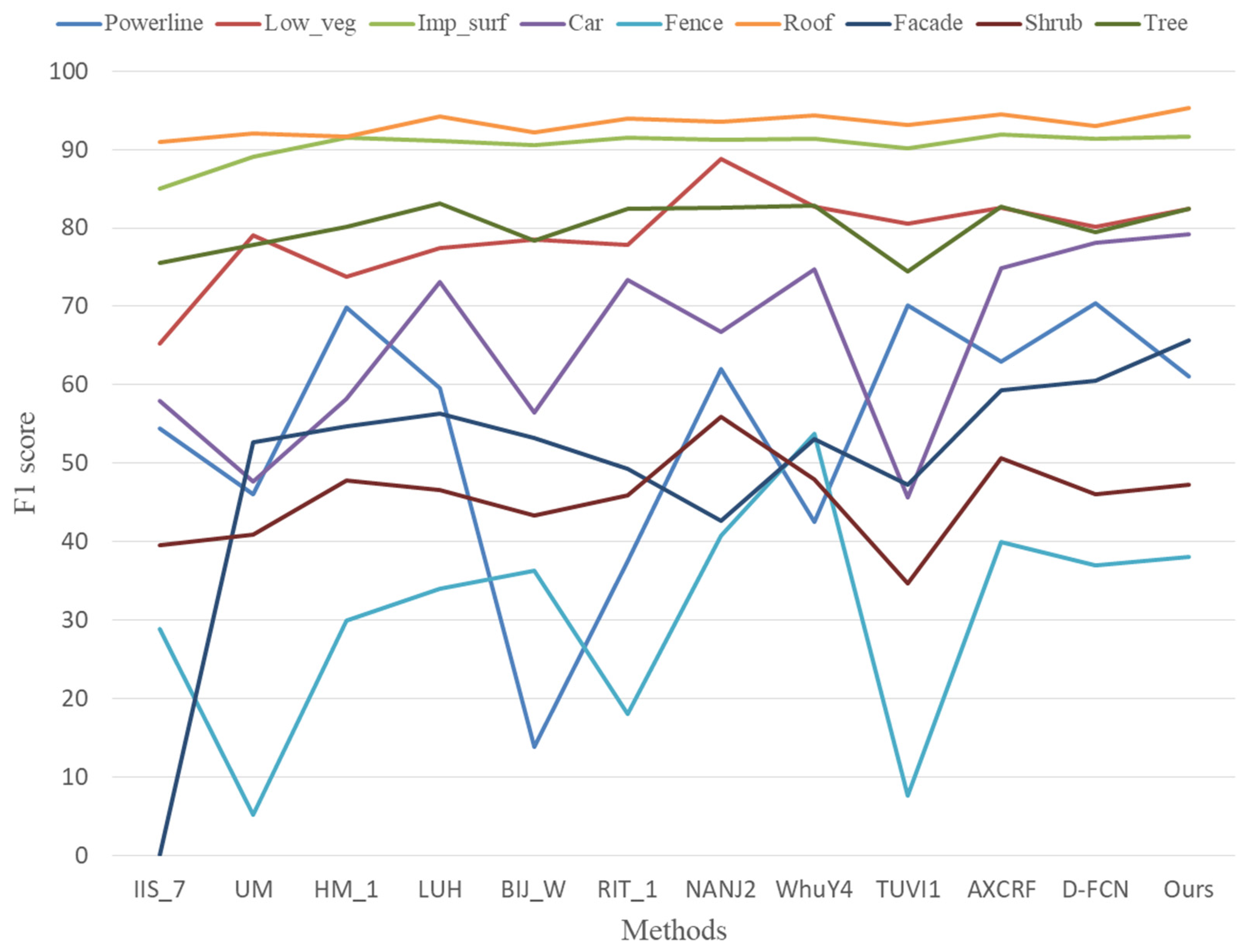
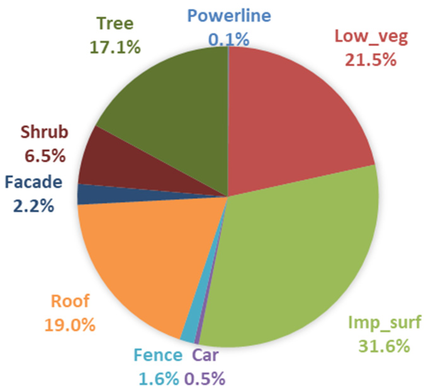
In order to analyze the performance of these methods in each category more intuitively, Table 5 was transformed into Figure 11. The number of points in each category of training set in Table 2 were also converted into percentages, and then transformed into Figure 12. Through the analysis of Figure 11 and Figure 12, we found that although the number of points in roof was not the largest, accounting for only 19% of the training set, all methods performed best on roof. Our method achieved the highest F1 score, which is 95.3%. All methods performed well on Imp_surf, which had the most points in the training set, and the F1 score was basically around 90%. They also had good performance on Low_veg and Tree, the F1 score basically reaching about 80%. These four categories had a large number of points in the training set, which enabled them to achieve higher classification accuracy. The experiments showed that, regardless of whether the method used was based on traditional machine learning or deep learning, higher classification accuracy could usually be obtained for those categories which accounted for a larger proportion in the training data. Surprisingly, although powerline and car accounted for a small proportion in the training set, some methods still performed well. The F1 score of our method on car was even close to 80%. The F1 score of most algorithms on facade was basically 60. The performance on fence and shrub was the worst. This is mainly because there were few points in these two categories, and their characteristics were very close to each other, which made it very difficult to distinguish them.

Figure 11. F1 score for each category of different methods in Vaihingen 3D data.

Figure 12. Category distribution of training set in Vaihingen 3D data.

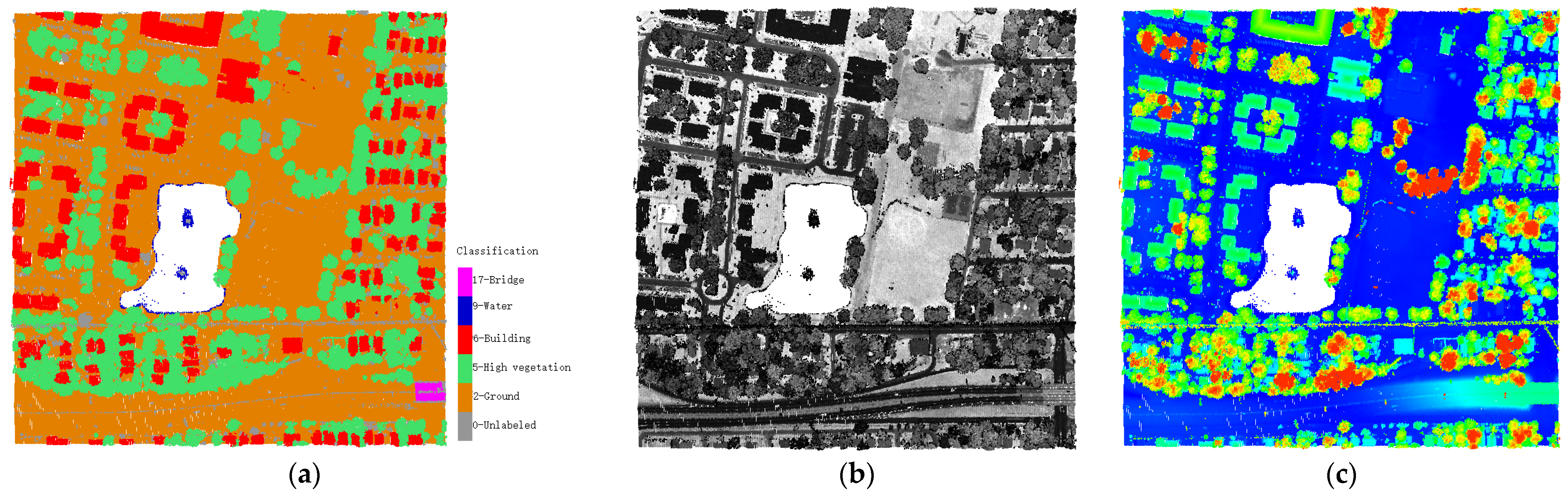
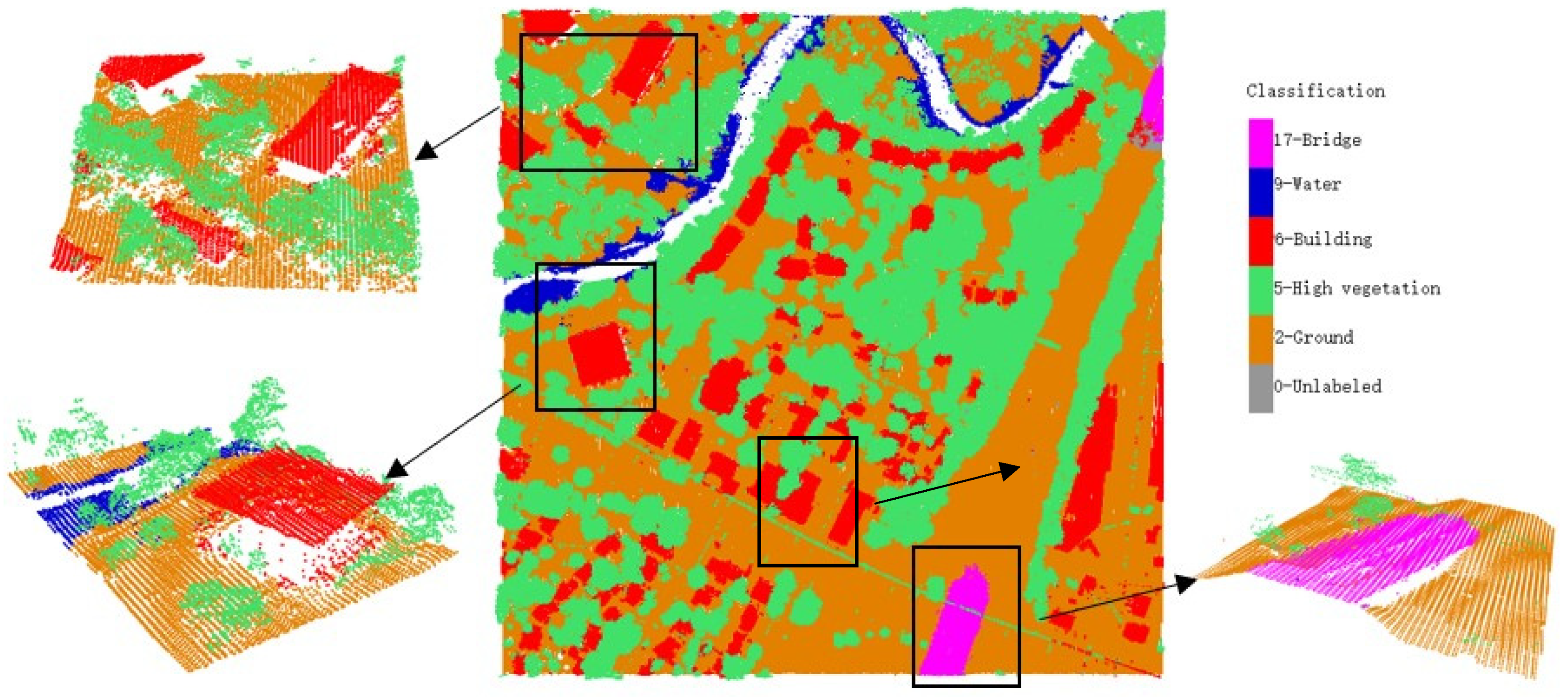
The classification confusion matrix for all the 10 tiles of DFC 3D test set is shown in Table 6. We performed best on ground and high vegetation, which had the most points in the training set according to Table 3. For water and bridge deck, although the number of points was very small in the training set, high IoU were still obtained. The water and bridge deck were mainly confused with the ground. According to Table 6, some building points are wrongly classified as ground and high vegetation, and some points belonging to the ground and high vegetation are mistakenly classified as buildings. This led to a reduction in IoU in the building category. Through further analysis of the results, we could see that most points with incorrect classification were located near the boundaries of adjacent objects, rather than inside them. This means that our method has a good label consistency and low classification noise.

Table 6. The confusion matrix of our method on the DFC 3D test set.

Predicted→↓Reference	Ground	High_veg	Building	Water	Bridge
Ground	5,104,677	18	11,119	10,147	4,789
High_veg	1540	1,344,385	28,499	14	0
Building	88,447	17,299	1,278,643	21	58
Water	6090	0	7	188,383	0
Bridge	7415	0	539	0	80,096
IoU	0.9750	0.9654	0.8943	0.9197	0.8468

Table 7 shows the quantitative comparison of performance between our method and other methods on the DFC 3D dataset. The first two columns of Table 7 show the OA and mIoU. The last five columns show the IoU for each category. As shown in Table 7, our method ranked first on the contest website with an OA of 97.74% and mIoU of 0.9202. As far as a single category is concerned, our method performed best in terms of ground, high vegetation and building. Because there was no specific information about these methods, except the name on the competition website of the DFC 3D data, there was no way to know what methods they used and make further comparisons. Although the data of the DFC 3D dataset were much larger than those of the Vaihingen 3D dataset, our algorithm still performed well. This shows that our method is suitable for the classification of point cloud in complicated and large-scale scenes.

Table 7. Quantitative comparison of performance between our method and other methods on the DFC 3D dataset. The highest scores are typed in bold.

Method	OA	mIoU	Ground	High_veg	Building	Water	Bridge
uang	96.39	0.8224	0.9563	0.9635	0.8426	0.9668	0.3827
piter	96.58	0.8603	0.9606	0.9541	0.8627	0.7640	0.7603
yky	96.14	0.8644	0.9551	0.9541	0.8324	0.8351	0.7456
aikin	97.18	0.8808	0.9680	0.9568	0.8832	0.7456	0.8506
brch	96.76	0.8899	0.9649	0.9477	0.8627	0.8674	0.8069
jinhou	97.52	0.8981	0.9737	0.9533	0.8949	0.8189	0.8497
raomb	96.84	0.9043	0.9664	0.9455	0.8572	0.9195	0.8330
rbync	97.37	0.8996	0.9728	0.9478	0.8814	0.9217	0.7747
Ours	97.74	0.9202	0.9750	0.9654	0.8943	0.9197	0.8468

6. Conclusions

In this paper, we proposed a novel CNN to classify airborne laser scanning point clouds without transformation to a 2D image or 3D voxel. We first designed a convolution operation for the unstructured and unordered points to learn the local features in a small area. Then, using an encoder and decoder structure similar to U-net, the classification network was constructed by stacking multiple convolution layers. The hierarchical features were learned efficiently and robustly. The class label was predicted for each point in an end-to-end manner. In order to evaluate the performance of the proposed method, we carried out experiments on the ISPRS Vaihingen 3D dataset and 2019 IEEE GRSS DFC 3D dataset. For the Vaihingen 3D dataset, we achieved an overall accuracy of 84.6% and average F1 score of 71.4%, which ranked fourth and first in the comparison of different methods. In particular, we obtained the highest F1 score for car, roof and facade. After evaluating our method on the DFC 3D dataset, we got an overall accuracy of 97.74% and mIoU of 0.9202, ranking first on the contest website. Our method performed best on ground, high vegetation and building. The experimental results show that this method has achieved state-of-the-art performance in the classification of airborne laser scanning point clouds, especially in complex large-scale scenes.

References

1. Axelsson, P. DEM generation from laser scanner data using adaptive TIN models. Int. Arch. Photogramm. Remote Sens. XXXIII 2000, 33, 110–117. [Google Scholar]
2. Hu, X.Y.; Yuan, Y. Deep-Learning-Based Classification for DTM Extraction from ALS Point Cloud. Remote Sens. 2016, 8, 730. [Google Scholar] [CrossRef] [Green Version]
3. Rottensteiner, F.; Sohn, G.; Gerke, M.; Wegner, J.D.; Breitkopf, U.; Jung, J. Results of the ISPRS benchmark on urban object detection and 3D building reconstruction. ISPRS J. Photogramm. Remote Sens. 2014, 93, 256–271. [Google Scholar] [CrossRef]
4. Awrangjeb, M.; Fraser, C.S. Automatic Segmentation of Raw LIDAR Data for Extraction of Building Roofs. Remote Sens. 2014, 6, 3716–3751. [Google Scholar] [CrossRef] [Green Version]
5. Hu, X.; Li, Y.; Shan, J.; Zhang, J.; Zhang, Y. Road Centerline Extraction in Complex Urban Scenes From LiDAR Data Based on Multiple Features. IEEE Trans. Geosci. Remote Sens. 2014, 52, 7448–7456. [Google Scholar] [CrossRef]
6. Hui, Z.; Hu, Y.; Jin, S.; Yevenyo, Y.Z. Road centerline extraction from airborne LiDAR point cloud based on hierarchical fusion and optimization. ISPRS J. Photogramm. Remote Sens. 2016, 118, 22–36. [Google Scholar] [CrossRef]
7. Kaartinen, H.; Hyyppa, J.; Yu, X.W.; Vastaranta, M.; Hyyppa, H.; Kukko, A.; Holopainen, M.; Heipke, C.; Hirschmugl, M.; Morsdorf, F.; et al. An International Comparison of Individual Tree Detection and Extraction Using Airborne Laser Scanning. Remote Sens. 2012, 4, 950–974. [Google Scholar] [CrossRef] [Green Version]
8. Zhen, Z.; Quackenbush, L.J.; Zhang, L.J. Trends in Automatic Individual Tree Crown Detection and Delineation-Evolution of LiDAR Data. Remote Sens. 2016, 8, 333. [Google Scholar] [CrossRef] [Green Version]
9. Sohn, G.; Jwa, Y.; Kim, H.B. Automatic powerline scene classification and reconstruction using airborne LiDAR data. ISPRS Ann. Photogramm. Remote Sens. Spat. Inf. Sci. 2012, I-3, 167–172. [Google Scholar] [CrossRef] [Green Version]
10. Ortega, S.; Trujillo, A.; Santana, J.M.; Suárez, J.P.; Santana, J. Characterization and modeling of power line corridor elements from LiDAR point clouds. ISPRS J. Photogramm. Remote Sens. 2019, 152, 24–33. [Google Scholar] [CrossRef]
11. Weinmann, M.; Urban, S.; Hinz, S.; Jutzi, B.; Mallet, C. Distinctive 2D and 3D features for automated large-scale scene analysis in urban areas. Comput. Graph. 2015, 49, 47–57. [Google Scholar] [CrossRef]
12. Weinmann, M.; Jutzi, B.; Hinz, S.; Mallet, C. Semantic point cloud interpretation based on optimal neighborhoods, relevant features and efficient classifiers. ISPRS J. Photogramm. Remote Sens. 2015, 105, 286–304. [Google Scholar] [CrossRef]
13. Guo, B.; Huang, X.; Zhang, F.; Sohn, G. Classification of airborne laser scanning data using JointBoost. ISPRS J. Photogramm. Remote Sens. 2015, 100, 71–83. [Google Scholar] [CrossRef]
14. Zhang, Z.; Zhang, L.; Tong, X.; Mathiopoulos, P.T.; Guo, B.; Huang, X.; Wang, Z.; Wang, Y. A Multilevel Point-Cluster-Based Discriminative Feature for ALS Point Cloud Classification. IEEE Trans. Geosci. Remote Sens. 2016, 54, 3309–3321. [Google Scholar] [CrossRef]
15. Dong, W.; Lan, J.; Liang, S.; Yao, W.; Zhan, Z. Selection of LiDAR geometric features with adaptive neighborhood size for urban land cover classification. Int. J. Appl. Earth Obs. 2017, 60, 99–110. [Google Scholar] [CrossRef]
16. Lodha, S.K.; Kreps, E.J.; Helmbold, D.P.; Fitzpatrick, D. Aerial LiDAR Data Classification Using Support Vector Machines (SVM). In Proceedings of the 3rd International Symposium on 3D Data Processing, Visualization and Transmission (3DPVT 2006), Chapel Hill, NC, USA, 14–16 June 2006. [Google Scholar] [CrossRef] [Green Version]
17. Mallet, C.; Bretar, F.; Roux, M.; Soergel, U.; Heipke, C. Relevance assessment of full-waveform lidar data for urban area classification. ISPRS J. Photogramm. Remote Sens. 2011, 66, S71–S84. [Google Scholar] [CrossRef]
18. Ghamisi, P.; Höfle, B. LiDAR Data Classification Using Extinction Profiles and a Composite Kernel Support Vector Machine. IEEE Geosci. Remote Sens. Lett. 2017, 14, 659–663. [Google Scholar] [CrossRef]
19. Guo, L.; Chehata, N.; Mallet, C.; Boukir, S. Relevance of airborne lidar and multispectral image data for urban scene classification using Random Forests. ISPRS J. Photogramm. Remote Sens. 2011, 66, 56–66. [Google Scholar] [CrossRef]
20. Ni, H.; Lin, X.; Zhang, J. Classification of ALS Point Cloud with Improved Point Cloud Segmentation and Random Forests. Remote Sens. 2017, 9, 288. [Google Scholar] [CrossRef] [Green Version]
21. Lodha, S.K.; Fitzpatrick, D.M.; Helmbold, D.P. Aerial Lidar Data Classification using AdaBoost. In Proceedings of the Sixth International Conference on 3-D Digital Imaging and Modeling (3DIM 2007), Montreal, QC, Canada, 21–23 August 2007; pp. 435–442. [Google Scholar]
22. Gerke, M.; Xiao, J. Fusion of airborne laserscanning point clouds and images for supervised and unsupervised scene classification. ISPRS J. Photogramm. Remote Sens. 2014, 87, 78–92. [Google Scholar] [CrossRef]
23. Zhu, Q.; Li, Y.; Hu, H.; Wu, B. Robust point cloud classification based on multi-level semantic relationships for urban scenes. ISPRS J. Photogramm. Remote Sens. 2017, 129, 86–102. [Google Scholar] [CrossRef]
24. Luo, H.; Wang, C.; Wen, C.; Zai, D.; Yu, Y.; Li, J. Semantic Labeling of Mobile LiDAR Point Clouds via Active Learning and Higher Order MRF. IEEE Trans. Geosci. Remote Sens. 2018, 56, 3631–3644. [Google Scholar] [CrossRef]
25. Niemeyer, J.; Rottensteiner, F.; Soergel, U. Contextual classification of lidar data and building object detection in urban areas. ISPRS J. Photogramm. Remote Sens. 2014, 87, 152–165. [Google Scholar] [CrossRef]
26. Vosselman, G.; Coenen, M.; Rottensteiner, F. Contextual segment-based classification of airborne laser scanner data. ISPRS J. Photogramm. Remote Sens. 2017, 128, 354–371. [Google Scholar] [CrossRef]
27. Wen, C.; Yang, L.; Li, X.; Peng, L.; Chi, T. Directionally constrained fully convolutional neural network for airborne LiDAR point cloud classification. Isprs J. Photogramm. Remote Sens. 2020, 162, 50–62. [Google Scholar] [CrossRef] [Green Version]
28. Krizhevsky, A.; Sutskever, I.; Hinton, G.E. Imagenet classification with deep convolutional neural networks. Adv. Neural Inf. Process. Syst. 2012, 25, 1097–1105. [Google Scholar] [CrossRef]
29. Szegedy, C.; Liu, W.; Jia, Y.; Sermanet, P.; Reed, S.; Anguelov, D.; Erhan, D.; Vanhoucke, V.; Rabinovich, A. Going deeper with convolutions. In Proceedings of the IEEE Conference on Computer Vision and Pattern Recognition, Boston, MA, USA, 7–12 June 2015; pp. 1–9. [Google Scholar]
30. He, K.; Zhang, X.; Ren, S.; Sun, J. Deep residual learning for image recognition. In Proceedings of the IEEE Conference on Computer Vision and Pattern Recognition, Las Vegas, NV, USA, 27–30 June 2016; pp. 770–778. [Google Scholar]
31. Long, J.; Shelhamer, E.; Darrell, T. Fully convolutional networks for semantic segmentation. In Proceedings of the IEEE Conference on Computer Vision and Pattern Recognition, Boston, MA, USA, 7–12 June 2015; pp. 3431–3440. [Google Scholar]
32. Ronneberger, O.; Fischer, P.; Brox, T. U-net: Convolutional networks for biomedical image segmentation. In Proceedings of the International Conference on Medical Image Computing and Computer-Assisted Intervention, Munich, Germany, 5–9 October 2015; pp. 234–241. [Google Scholar]
33. Chen, L.-C.; Papandreou, G.; Kokkinos, I.; Murphy, K.; Yuille, A.L. Deeplab: Semantic image segmentation with deep convolutional nets, atrous convolution, and fully connected crfs. IEEE Trans. Pattern Anal. Mach. Intell. 2017, 40, 834–848. [Google Scholar] [CrossRef]
34. Yang, Z.; Jiang, W.; Xu, B.; Zhu, Q.; Jiang, S.; Huang, W. A Convolutional Neural Network-Based 3D Semantic Labeling Method for ALS Point Clouds. Remote Sens. 2017, 9, 936. [Google Scholar] [CrossRef] [Green Version]
35. Zhao, R.; Pang, M.; Wang, J. Classifying airborne LiDAR point clouds via deep features learned by a multi-scale convolutional neural network. Int. J. Geogr. Inf. Sci. 2018, 32, 960–979. [Google Scholar] [CrossRef]
36. Huang, J.; You, S. Point Cloud Labeling using 3D Convolutional Neural Network. In Proceedings of the International Conference on Pattern Recognition, Cancun, Mexico, 4–8 December 2016; pp. 2670–2675. [Google Scholar]
37. Rizaldy, A.; Persello, C.; Gevaert, C.; Oude Elberink, S.; Vosselman, G. Ground and Multi-Class Classification of Airborne Laser Scanner Point Clouds Using Fully Convolutional Networks. Remote Sens. 2018, 10, 1723. [Google Scholar] [CrossRef] [Green Version]
38. Wang, Z.; Zhang, L.; Zhang, L.; Li, R.; Zheng, Y.; Zhu, Z. A Deep Neural Network With Spatial Pooling (DNNSP) for 3-D Point Cloud Classification. IEEE Trans. Geosci. Remote Sens. 2018, 56, 4594–4604. [Google Scholar] [CrossRef]
39. Yousefhussien, M.; Kelbe, D.J.; Lentilucci, E.J.; Salvaggio, C. A multi-scale fully convolutional network for semantic labeling of 3D point clouds. ISPRS J. Photogramm. Remote Sens. 2018, 143, 191–204. [Google Scholar] [CrossRef]
40. Winiwarter, L.; Mandlburger, G.; Schmohl, S.; Pfeifer, N. Classification of ALS Point Clouds Using End-to-End Deep Learning. PFG J. Photogramm. Remote Sens. Geoinf. Sci. 2019, 87, 75–90. [Google Scholar] [CrossRef]
41. Arief, H.A.A.; Indahl, U.G.; Strand, G.-H.; Tveite, H. Addressing overfitting on point cloud classification using Atrous XCRF. ISPRS J. Photogramm. Remote Sens. 2019, 155, 90–101. [Google Scholar] [CrossRef] [Green Version]
42. Soilan, M.; Riveiro, B.; Balado, J.; Arias, P. Comparison of heuristic and deep learning-based methods for ground classification from aerial point clouds. Int. J. Digit. Earth 2020, 13, 1115–1134. [Google Scholar] [CrossRef]
43. Huang, R.; Xu, Y.; Stilla, U. GraNet: Global relation-aware attentional network for semantic segmentation of ALS point clouds. ISPRS J. Photogramm. Remote Sens. 2021, 177, 1–20. [Google Scholar] [CrossRef]
44. Lin, Y.; Vosselman, G.; Cao, Y.; Yang, M.Y. Local and global encoder network for semantic segmentation of Airborne laser scanning point clouds. ISPRS J. Photogramm. Remote Sens. 2021, 176, 151–168. [Google Scholar] [CrossRef]
45. Lodha, S.K.; Fitzpatrick, D.M.; Helmbold, D.P. Aerial lidar data classification using expectation-maximization. Proc. SPIE Int. Soc. Opt. Eng. 2007, 6499, 64990L. [Google Scholar] [CrossRef] [Green Version]
46. Chehata, N.; Guo, L.; Mallet, C. Airborne lidar feature selection for urban classification using random forests. Int. Arch. Photogramm. Remote Sens. Spat. Inf. Sci. 2009, 38, W8. [Google Scholar]
47. Qi, C.R.; Su, H.; Mo, K.; Guibas, L.J. PointNet: Deep Learning on Point Sets for 3D Classification and Segmentation. arXiv 2016, arXiv:1612.00593. [Google Scholar]
48. Qi, C.R.; Yi, L.; Su, H.; Guibas, L.J. PointNet++: Deep Hierarchical Feature Learning on Point Sets in a Metric Space. arXiv 2017, arXiv:1706.02413. [Google Scholar]
49. Li, Y.; Bu, R.; Sun, M.; Wu, W.; Di, X.; Chen, B. PointCNN: Convolution on χ-Transformed Points. arXiv 2018, arXiv:1801.07791. [Google Scholar]
50. Mingyang, J.; Yiran, W.; Cewu, L. PointSIFT: A SIFT-like network module for 3D point cloud semantic segmentation. arXiv 2018, arXiv:1807.00652. [Google Scholar]
51. Thomas, H.; Qi, C.R.; Deschaud, J.; Marcotegui, B.; Goulette, F.; Guibas, L. KPConv: Flexible and Deformable Convolution for Point Clouds. In Proceedings of the 2019 IEEE/CVF International Conference on Computer Vision (ICCV), Seoul, Korea, 27 October–2 November 2019; pp. 6410–6419. [Google Scholar]
52. Boulch, A. ConvPoint: Continuous convolutions for point cloud processing. Comput. Graph. 2020, 88, 24–34. [Google Scholar] [CrossRef] [Green Version]
53. Wu, W.; Qi, Z.; Fuxin, L. PointConv: Deep Convolutional Networks on 3D Point Clouds. In Proceedings of the 2019 IEEE/CVF Conference on Computer Vision and Pattern Recognition (CVPR), Long Beach, CA, USA, 15–20 June 2019; pp. 9613–9622. [Google Scholar]
54. Hu, Q.; Yang, B.; Xie, L.; Rosa, S.; Guo, Y.; Wang, Z.; Trigoni, N.; Markham, A. RandLA-Net: Efficient Semantic Segmentation of Large-Scale Point Clouds. In Proceedings of the 2020 IEEE/CVF Conference on Computer Vision and Pattern Recognition (CVPR), Seattle, WA, USA, 13–19 June 2020; pp. 11105–11114. [Google Scholar] [CrossRef]
55. Guo, Y.; Wang, H.; Hu, Q.; Liu, H.; Liu, L.; Bennamoun, M. Deep Learning for 3D Point Clouds: A Survey. IEEE Trans. Pattern Anal. Mach. Intell. 2020. [Google Scholar] [CrossRef]
56. Armeni, I.; Sener, O.; Zamir, A.R.; Jiang, H.; Brilakis, I.; Fischer, M.; Savarese, S. 3D Semantic Parsing of Large-Scale Indoor Spaces. In Proceedings of the 2016 IEEE Conference on Computer Vision and Pattern Recognition (CVPR), Las Vegas, NV, USA, 27–30 June 2016; pp. 1534–1543. [Google Scholar]
57. Dai, A.; Chang, A.X.; Savva, M.; Halber, M.; Funkhouser, T.; Nießner, M. ScanNet: Richly-Annotated 3D Reconstructions of Indoor Scenes. In Proceedings of the 2017 IEEE Conference on Computer Vision and Pattern Recognition (CVPR), Honolulu, HI, USA, 21–26 July 2017; pp. 2432–2443. [Google Scholar]
58. Bosch, M.; Foster, K.; Christie, G.; Wang, S.; Hager, G.D.; Brown, M. Semantic Stereo for Incidental Satellite Images. In Proceedings of the 2019 IEEE Winter Conference on Applications of Computer Vision (WACV), Waikoloa Village, HI, USA, 7–11 January 2019; pp. 1524–1532. [Google Scholar]
59. Saux, B.; Yokoya, N.; Hänsch, R.; Brown, M. 2019 IEEE GRSS Data Fusion Contest: Large-Scale Semantic 3D Reconstruction [Technical Committees]. IEEE Geosci. Remote Sens. Mag. 2019, 7, 33–36. [Google Scholar] [CrossRef]
60. Ramiya, A.M.; Nidamanuri, R.R.; Ramakrishnan, K. A supervoxel-based spectro-spatial approach for 3D urban point cloud labelling. Int. J. Remote Sens. 2016, 37, 4172–4200. [Google Scholar] [CrossRef]
61. Horvat, D.; Žalik, B.; Mongus, D. Context-dependent detection of non-linearly distributed points for vegetation classification in airborne LiDAR. ISPRS J. Photogramm. Remote Sens. 2016, 116, 1–14. [Google Scholar] [CrossRef]
62. Niemeyer, J.; Rottensteiner, F.; Soergel, U.; Heipke, C. Hierarchical Higher Order Crf for the Classification of Airborne Lidar Point Clouds in Urban Areas. ISPRS Int. Arch. Photogramm. Remote Sens. Spat. Inf. Sci. 2016, 41, 655–662. [Google Scholar] [CrossRef] [Green Version]
Publisher’s Note: MDPI stays neutral with regard to jurisdictional claims in published maps and institutional affiliations.
Article Metrics
Citations
Article Access Statistics
Multiple requests from the same IP address are counted as one view.