Abstract
Accurate modeling and simulation of lower limb rehabilitation exoskeleton (LLRE) enables effective control resulting in enhanced performance and ensuring efficient rehabilitation. There are two primary objectives of this study. First is to validate the existing models and second is to identify the optimal modeling approach for exoskeletons. For validation, firstly a lower limb rehabilitation exoskeleton is modeled using three different modeling approaches which include analytical modeling, bond graph modeling, and modeling through Simscape (SS). Thereafter, dynamic responses of analytical and graphical modeling are compared with SS model using key dynamic response parameters, including rise time, peak time, and others. The SS-based physical model can be employed for validation because SS, unlike mathematical modeling, uses unit-consistent physical domain data and, therefore, serves as an intermediate step between mathematical modeling and hardware validation. Secondly, to identify the most suitable modeling approach, a structured and comprehensive comparison of different modeling approaches based on aspects such as control domain, complexity, ease of use, and other relevant factors is carried out. The results highlight the qualitative strengths and limitations of the three approaches. Previous studies focus on individual methods and lack such comparison. This work contributes to the validation of models and identification of an efficient and effective modeling methodology for LLRE. The findings reveal that Simscape™ is the most suitable approach for modeling LLREs as it provides multidisciplinary system modeling and supports real-time simulation. The validated model can now be employed for advancements in model-based control design. Moreover, the identified optimal approach provides an insight to researchers and engineers for model selection in early-stage design and control development of complex mechatronic systems. Future work includes comparison of dynamic responses with actual hardware responses to experimentally validate the effectiveness of the model for real-world patient assistance and mobility restoration.
1. Introduction
The world population is increasing and along with it, the number of patients with musculoskeletal and neuro-motor dysfunction is rising at a rapid pace. Both dysfunctions cause lower limb-related disabilities that limit patients’ mobility. Immobility of patients makes them vulnerable to other diseases such as cardio-vascular and diabetes. Old age is another factor that causes immobility. Most people in old age experience common diseases such as sarcopenia, weak bones, and reduced joint performance, resulting in poor health conditions and restriction in their movements [1,2]. The number of people aged 65 or above in 2050 is estimated to reach around 1549 million, which is almost a 120% increase from the current figures [3]. During the COVID-19 pandemic, elderly and disabled people faced difficulties in seeking help due to strict lockdowns and social distancing policies. Elderly people were at greater risk while seeking assistance as they were more susceptible to the corona virus [4,5,6]. Due to the abovementioned facts, proper rehabilitation and care methods are necessary to improve patients’ mobility and reduce dependence on foreign assistance.
Traditional rehabilitation methods have a few drawbacks, including lack of versatility to address patients’ specific needs, and successful rehabilitation is bound by the experience of physicians. Patients typically opt to exercise at home due to the extended duration of therapy and hefty expenditures, but this type of training lacks scientific guidelines. Under these circumstances and without proper rehabilitation, many patients lose their ability to stand up on their feet again. The use of advanced rehabilitation equipment is an effective option for regaining lower limb function and control. Rehabilitation using state-of-the-art techniques can help alleviate pain, increase productivity, boost self-confidence, and improve overall quality of life.
As a result, there is a growing demand for more convenient rehabilitation robots to aid in the recovery process. Advancements in robotic technology offer an opportunity for lower extremity rehabilitation to potentially boost therapeutic dosage while relieving some of the physiotherapist’s responsibilities [7,8]. Wearable lower limb exoskeleton has become a well sought mechatronic system for research due to its promising benefits in terms of assistance and rehabilitation for disabled and elderly people. Robotic systems can facilitate joint mobility, provide sensory feedback during movement, and offer a secure environment for controlled parameter variations [9]. While patients have a positive attitude towards the use of robotic exoskeletons in rehabilitation [7], a therapist’s willingness to employ robotic technology in their practice may be influenced by the learning curve required to grow accustomed to using the device and the lack of scientific data supporting its therapeutic benefits [10,11].
Lower limb rehabilitation exoskeletons (LLREs) can serve a wide range of patients suffering from spinal cord injury, stroke, cerebral palsy, Parkinson, multiple sclerosis, and traumatic brain injury. Rehabilitation robots, such as LLREs, can assist therapists in reducing their workload, analyzing training data, and evaluating recovery in a controlled and reproducible manner [12]. The exoskeletons have been designed and studied since the 1960s, but technical limitations prevented them from achieving their intended objectives. Functional classification of exoskeletons based on their applications related to rehabilitation of the lower limb is shown in Figure 1. Within the medical domain, exoskeletons are designed for upper limb and lower limb rehabilitation. LLREs are further categorized based on their usage in two primary settings: stationary and mobile. Stationary exoskeletons refer to exoskeletons integrated into fixed platforms combined with treadmill and body weight support systems whereas mobile exoskeletons refer to rehabilitation systems which provide on-ground training either independently or with mobile platforms. This research focuses on the modeling and simulation of mobile LLREs. The category of mobile exoskeletons is highlighted in Figure 1 to emphasize the scope of the present work.
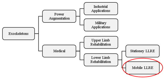
Figure 1.
Classification of exoskeletons highlighting mobile exoskeletons−the focus of this study.
Researchers have developed various hardware models for lower limb rehabilitation exoskeletons (LLREs) with the goal of developing better exoskeletons for improved rehabilitation results. Some earlier models, such as those in [13,14,15], only had 2 degrees of freedom (DOF) for each leg (hip and knee), with the ankle fixed in place, making it easier to control but less conformant to the human body. More recent models, such as those in [16,17,18,19,20,21], have 3 DOF for each leg, including an ankle joint, which better conforms to human anatomy and enhances balance during assisted walking.
DC motors have been the preferred choice for actuation in most proposed models due to their compact size, ease of control, accuracy, and repeatability. However, a few models in [22,23] have used hydraulic and pneumatic actuators, which can deliver higher torque but are less accurate, require bulky equipment, and are difficult to control.
To develop the exoskeleton model, dynamic modeling of the physical system is carried out. In previous studies, it has been observed that researchers have performed dynamic modeling of various LLREs by using different modeling techniques. They have performed dynamic modeling and simulation of rehabilitation exoskeletons using Euler–Lagrange (EL)/Euler–Newton (EN) method and bond graph modeling technique [13,16,24,25,26,27,28,29,30]. Table 1 summarizes the modeling techniques used in the past for obtaining the mathematical model of LLREs and other bio-mechatronic systems.

Table 1.
Overview of dynamic modeling approaches.
In the Euler–Lagrange method, the difference between the kinetic and potential energies is used to generate a system model while relating the associated forces to the generalized coordinates. Although a controller can be designed for the modeled system to obtain the desired output, this method involves complex computations to precisely model the errors and inaccuracies. In addition to that, the EL method is less flexible in terms of handling any changes or modifications in mechanical hardware. For any change in hardware model, the modeling process requires re-derivation of all equations, increasing the computational load. An alternative modeling approach for manipulators is the bond graph (BG) technique which provides a simple and flexible model of the system [36,37,38,39,40,41] as compared to the conventional Lagrangian method. Using BG method, a comprehensive modeling of any mechatronics system can be performed. In research works [40,41,42], modeling of exoskeletons for medical and industrial purposes is performed using the BG method.
Modeling of exoskeletons can be carried out using the Simscape (SS). It is a modeling tool that allows efficient modeling of complex physical systems within the Simulink environment. The modeling process is facilitated using physical connections, and the models built are based on physical components and their interactions through energy flow. The physical network approach provides an intuitive and comprehensible way of modeling complex systems involving multiple physical domains such as electrical, hydraulic, mechanical, thermal, and more. Furthermore, there are a variety of pre-built components that can be easily assembled into models. The pre-built components save time and effort when developing a model and ensure its accuracy and reliability.
Once a model has been created in SS, it can be simulated and analyzed using the same methods and tools as Simulink. SS offers a variety of analysis tools for investigating the behavior of a system, such as time-domain simulation, frequency-domain analysis, and optimization.
Several modeling approaches, i.e., analytical, graphical, and physical, have been reviewed above. Despite significant achievements in the modeling of exoskeleton systems, previous studies primarily focused on individual modeling and lacked a structured and comprehensive comparison of modeling approaches. Such a comparison is essential in the identification of the most suitable modeling approach for LLRE. Consequently, it remains an open research challenge to select the most suitable modeling approach for multidomain systems that ensure accuracy, ease of use, and computational efficiency. Firstly, this work addresses the highlighted gap by providing a systematic and structured comparison of modeling approaches based on technical parameters, thereby validating the existing models. Secondly, through the comparison of qualitative aspects, this work contributes the identification of the optimized approach for the modeling of the LLRE. Together, these contributions reflect the novelty of this research work. The research methodology followed in this work is presented in Figure 2.
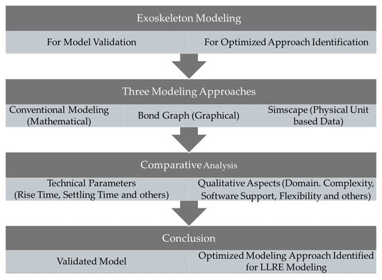
Figure 2.
Research methodology for model validation and optimized modeling approach identification for LLRE.
Exoskeleton modeling in this study was carried out using three modeling approaches, and the responses and approaches are compared based on technical parameters and qualitative aspects, respectively, resulting in the validation of existing models and identification of optimized modeling approach for LLRE. The validated model and the identified optimized approach will support researchers in the field of LLRE modeling and control in selecting a suitable modeling approach, enabling them to design efficient control algorithms.
This paper is organized as follows: The introduction section provides an overview of the different exoskeletons and modeling and simulation approaches for LLREs. Section 2 details the modeling and simulation of LLRE using three different modeling approaches. Section 3 presents the results and comparative analysis of the three approaches based on technical parameters and qualitative aspects. It further discusses the findings, highlights the advantages and limitations of each approach and ultimately identifies the most suitable modeling approach. Section 4 outlines the conclusions and future research directions.
2. Modeling and Simulation of LLRE
In this section, the details of the hardware of LLRE have been presented in detail, followed by a comprehensive modeling of the LLRE using three different approaches.
2.1. LLRE Hardware Components
The proposed LLRE has three DOF and consists of three links, where link 1 is aligned to the femur, link 2 with the fibula and tibia and link 3 with the foot. The hip, knee, and ankle joints are designed for flexion and extension. The maximum range of motion for the joints has been set at 30°/212° for the hip, 60°/210° for the knee, and 13°/220° for the ankle to ensure physiological comfort and safety. These joint angles belong to a local coordinate system of exoskeleton with neutral alignment set at 180°. Upon transforming these angles into clinical joint space, the ranges correspond to anatomical limits as established in [60,61] for hip, knee, and ankle joints. The exoskeleton system has 1 DOF movement for each joint (hip, knee, and ankle) with linear actuators. The CAD model and hardware of LLRE are shown in Figure 3.
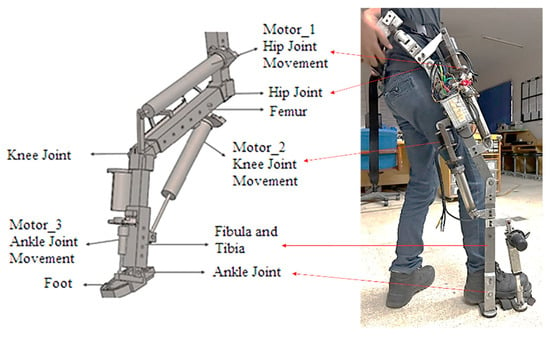
Figure 3.
CAD model and hardware of LLRE.
In the case of the motor mounted at the hip joint, the dynamic contributions of the connected structure—including two distal links (link 2 and link 3), two motors (motors for knee and ankle joint actuation), and the mass of a human leg—can be lumped and reflected towards the hip joint for modeling as a combined load, i.e., a spring–mass–damper acting on the hip motor. Such a model is an equivalent (reduced) dynamic representation and is referred to as a “composite model.” This abstraction captures the dynamic interaction between the actuator and the mechanical load for modeling and control purposes.
The composite model for hip joint control is considered. The schematic diagrams of the complete LLRE model and composite model are shown in Figure 4 and Figure 5, respectively. Figure 4 shows the schematic diagram of the LLRE. Three motors (mhj, mkj, and maj, i.e., motors for actuation of hip joint, knee joint, and ankle joint, respectively) along with rack and pinion mechanisms for achieving linear actuation are connected in parallel to the links which are connected using hinge joints. The damping and stiffness of the hinge joints are added in the model. Figure 5 shows the schematic diagram of the composite model presenting the linear actuator for hip joint actuation along with the rack and pinion and combined mass, damping, and stiffness from the distal links and motors as seen by the mhj. For the dynamic modeling of exoskeleton, two cases, i.e., exoskeletons with different values of system variables have been considered. The purpose of presenting two cases is to evaluate the dynamic behavior and robustness for different load conditions. The parameters for both cases are shown in Table 2.
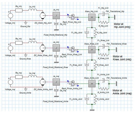
Figure 4.
Schematic diagram of complete LLRE model.

Figure 5.
Schematic diagram of composite model.

Table 2.
Parameters for dynamic modeling of LLRE.
2.2. Conventional Modeling of LLRE
In this section, a conventional model of the LLRE is developed using the laws of physics to deduce the equations for the system. The mechatronic system comprises a motor with gears, rack and pinion, and mass–spring–damper load as shown in Figure 5.
By applying Newton’s second law:
where ‘’ is moment of inertia of armature shaft, ‘’ is damping of armature shaft, ‘’ is the motor torque. For the spring–mass–damper system,
where ‘’ is the mass of the load attached to rack, ‘’ is viscous damping of the rack and pinion and ‘’ is the stiffness of the rack. can be written as
In Equation (3), ‘’ is the linear displacement of the load, ‘’ represents the radius of the pinion and ‘’ represents the angular displacement of the pinion. Substituting values from Equations (2) and (3) in Equation (1):
Using Kirchhoff’s Voltage Law (KVL),
where ‘’ is applied armature voltage, ‘’ is back EMF of motor, ‘’ and ‘’ are armature resistance and inductance, respectively. The back EMF voltage can be determined as
where ‘’ is the back EMF constant of DC motor. The torque generated by the motor can be expressed as
where ‘’ is the motor’s torque, ‘’ is the motor’s torque constant, and ‘’ is the motor’s armature current. Equation (7) can be written as
After substituting values in Equation (5) and re-writing,
Equation (9) becomes
The transfer function of the system in terms of the velocity of the load attached to the rack of the system and the voltage applied to the system is determined as Equation (12).
For the transfer function of exoskeleton case-I, the values of the variables from Table 2 are substituted into Equation (12). The open-loop and closed-loop transfer functions become
Similarly, for LLRE case-II, the transfer functions of the system become
2.3. Bond Graph Modeling of LLRE
In the previous section, the dynamic model in the form of transfer functions has been obtained in Equations (13)–(16). The relationship between the voltage ‘’ provided to the exoskeleton and the resulting limb displacement ‘’ can be analyzed. In this section, LLRE is modeled using the BG technique. BG enables researchers to better understand and evaluate the dynamics of the system by offering a more comprehensible and visual description of the system. Bond graph modeling further enables the inclusion of elements from multiple physical domains, such as mechanical, electrical, and hydraulic, providing a more flexible environment for system modeling. Bond graph modeling technique has been used in [45,46,47,48,49,50,51,52,53] for the modeling of various robotic systems. This approach is especially helpful for LLRE as the effects of parameter changes on the system’s behavior can be analyzed efficiently as compared to conventional modeling. 20-Sim software has been used as a tool for the generation of bond graph and for obtaining system equations in the form of state space. The word bond graph of the proposed exoskeleton is presented in Figure 6, illustrating the flow of electrical power from the source to the motor, followed by the flow of mechanical power for the desired rotation of the links.

Figure 6.
Word bond graph of proposed exoskeleton.
To obtain accurate modeling, real-time parametric values for both electrical and mechanical hardware have been employed. These include various parameters, such as the armature resistance of the motor, damping and inertia of the motor, and damping of links and joints. The BG of the complete LLRE and the composite model are shown in Figure 7 and Figure 8. The parametric values of exoskeleton hardware are listed in Table 2 with the two cases being considered. The transfer function of the bio-mechatronics system case-I is obtained after frequency response analysis in 20-Sim and is presented in Equation (17).
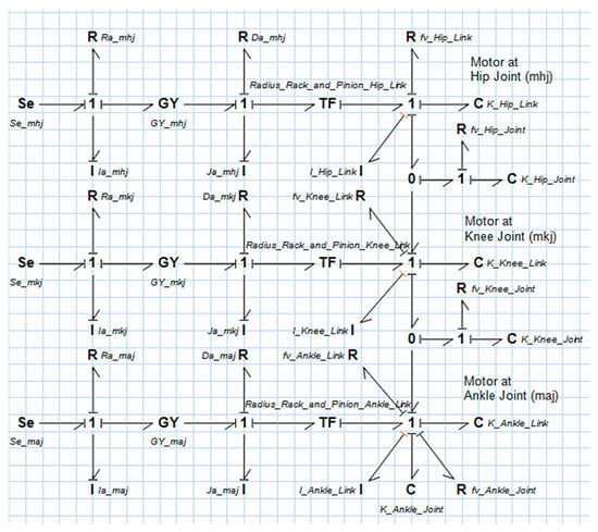
Figure 7.
Bond graph of LLRE using 20-Sim.
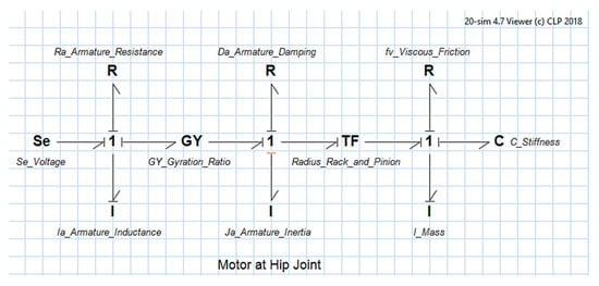
Figure 8.
Bond graph of composite model using 20-Sim.
The OL and CL transfer functions of case-I and case-II in Equation (13) through Equations (16) and (17) through Equation (20) are the same and will present similar system responses to the various given input signals.
2.4. SimscapeTM Model of LLRE
In this section, LLRE is modeled using Simscape. Multidomain components with physical signals are attached as per the schematic diagram and the system model is obtained. The controlled voltage source supplies the input voltage to the DC motor component which, according to the parametric values ( and ), converts the electrical energy to mechanical energy. The SS rack and pinion block converts the rotational motion to translational motion. The block named, “Simulink-PS Converter” converts the unitless numerical Simulink signal to a unit-based physical signal. Hence, bridging the gap between mathematical simulation and real hardware. The SS model of the complete LLRE is shown in Figure 9. The parametric values are obtained from Table 2, which were used for conventional mathematical modeling and bond graph modeling earlier. The equivalent composite model of the exoskeleton developed using SS is presented in Figure 10.
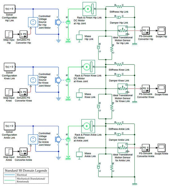
Figure 9.
SimscapeTM model of LLRE.
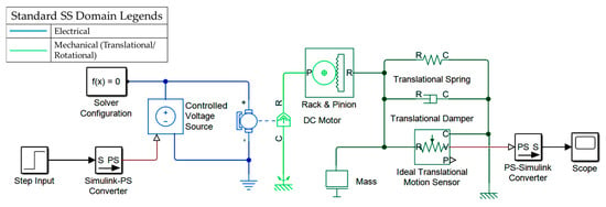
Figure 10.
SimscapeTM of composite model.
3. Results, Discussion, and Comparative Analysis
In this section, the dynamic responses of both cases of the LLRE obtained from CM, BG, and SS modeling approaches are presented and analyzed. Thereafter, the error between the responses obtained from CM and BG is compared with the SS modeling approach. This comparison will identify the differences between the models and, hence, will validate the existing model. Figure 11 and Figure 12 show the OL and CL step, impulse, and sinusoidal responses of the LLRE case-I and case-II. For CL, the feedback configuration employed is unity. No additional scaling or controller design is introduced at this stage as the objective is to compare the responses from different modeling approaches for validation. The comparison of OL and CL step, impulse, and sinusoidal (time-varying signal) responses will highlight the tracking performance, response to sudden disturbances, and phase lag, respectively, in models with and without feedback. The reason for analyzing the system dynamics for these signals is because they represent typical scenarios in rehabilitation robotics and efficient control design.
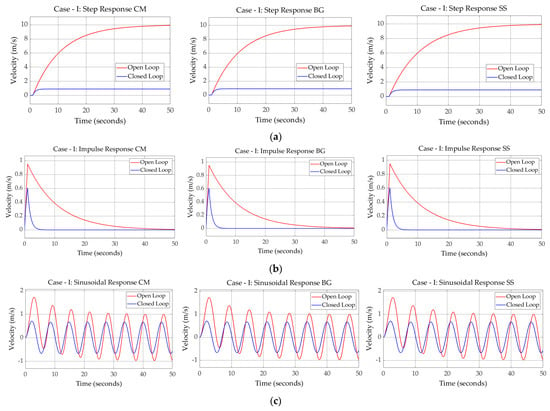
Figure 11.
Dynamic responses of LLRE case−I: (a) step responses: conventional, bond graph and Simscape model (left to right); (b) impulse Responses: conventional, bond graph and Simscape model (left to right); (c) sinusoidal responses: conventional, bond graph and Simscape model (left to right).
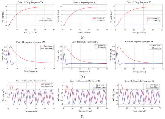
Figure 12.
Dynamic responses of LLRE case−II: (a) step responses: conventional, bond graph and Simscape model (left to right); (b) impulse responses: conventional, bond graph and Simscape model (left to right); (c) sinusoidal responses: conventional, bond graph and Simscape model (left to right).
3.1. Results and Discussion
3.1.1. Step Response—Open Loop and Closed Loop
The open-loop results provide significant insights into the inherent dynamic characteristics of the system without external control influence. As shown in Figure 11 and Figure 12, both models exhibit stable step responses without feedback control, reaching final values of 9.191 and 9.951, respectively. However, the OL response is slower in both cases, with a rise time of 21.2990 and 19.214 secs. The steady-state error and other values of the response parameters are shown in Table 3.

Table 3.
Details of response/performance parameters.
With unity feedback control, the CL response demonstrates faster rise time (9.394 s), reduced steady-state error (0.0910), and improved stability. The CL system outperforms the OL system, indicating better tracking performance and enhanced stability.
3.1.2. Impulse Response—Open Loop and Closed Loop
Both models peak at 1 s with a small difference in rise times (0.7918 and 0.7648 s). However, the OL system takes significantly longer (50 s) to settle at zero. The open-loop impulse response highlights the system’s natural damping characteristics and its ability to reject disturbances without feedback. The CL response shows faster settling (4.773 s).
3.1.3. Sinusoidal Response—Open Loop and Closed Loop
The OL system response to time-varying sinusoidal signal demonstrates poor trajectory tracking with noticeable amplitude deviations and phase lag.
The CL system exhibits better tracking accuracy with minimal phase lag and amplitude deviation, making it more suitable for trajectory tracking in rehabilitation applications. Closed-loop control consistently enhances system performance across step, impulse, and sinusoidal inputs by reducing steady-state error, improving settling time, and ensuring better tracking accuracy.
3.2. Comparative Analysis of Modeling Approaches
3.2.1. Dynamic Responses upon Technical Parameters
The comparative study of dynamic responses, i.e., of Euler–Lagrange vs. Simscape™ and bond graph vs. Simscape™ quantitatively confirms negligible error between the models. The values of all parameters are considered up to four decimal places, while error values fall in the range of exponent −7 and −13 as can be seen in Figure 13 and Figure 14, leading to their consideration as zero. The insignificance of minimal differences such as zero beyond seven decimal places fall within acceptable tolerances for LLRE. As for LLRE, reference trajectory tracking error is normally reduced to zero or less. While it has no specific value of precision, for factual accuracy, it can be correlated with a clinically acceptable range of errors in rehabilitation. Similarly, the clinically acceptable error is also not a universal number and is purpose specific. Therefore, an error of zero or less is acceptable in all circumstances. Furthermore, through robust, intelligent, and adaptive control strategies, an error of less than zero degree and precise up to three decimal places (i.e., ) can be achieved as presented in [62]. For even higher precision, further research and analysis can be conducted to identify the potential sources of discrepancy and refine the models accordingly. Therefore, the results confirm that the responses obtained from different modeling approaches do not vary from each other, thus validating the existing models.
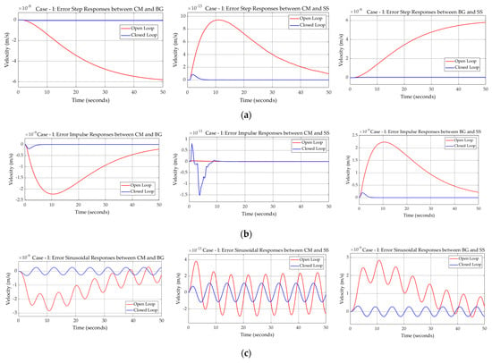
Figure 13.
Error between responses of models LLRE case−I: (a) step responses: conventional, bond graph and Simscape model (left to right); (b) impulse responses: conventional, bond graph and Simscape model (left to right); (c) sinusoidal responses: conventional, bond graph and Simscape model (left to right).
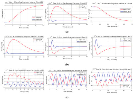
Figure 14.
Error between responses of models LLRE case−II: (a) step responses: conventional, bond graph and Simscape model (left to right); (b) impulse responses: conventional, bond graph and Simscape model (left to right); (c) sinusoidal responses: conventional, bond graph and Simscape model (left to right).
Each modeling approach has its strengths and limitations. The Euler–Lagrange method is widely used in classical mechanics, robotics, and control applications, offering a strong mathematical framework and requiring strong mathematical background. Bond graph modeling is greater in flexibility compared to EL and provides an intuitive visual representation of multidomain systems and requires familiarity with bond graph theory. Simscape™ is more flexible than graphical modeling and provides real-time simulation environment, making it a promising alternative for modeling of mechatronics systems such as LLRE.
3.2.2. Modeling Approaches upon Qualitative Aspects
For the comparative analysis of modeling approaches based on qualitative aspects, the qualitative aspects of the modeling approaches are first presented; thereafter, the aspects for each approach are scored using the Likert scale. Finally, the overall score for each approach is calculated. The qualitative aspects include domain, complexity, software support, flexibility, simulation speed, and ease of use. Table 4 presents the advantages and disadvantages of each modeling approach over the other for the different aspects.

Table 4.
Qualitative aspects of modeling approaches.
Table 5 shows the Likert scale score according to the rubrics defined in Table 6. The description of each score is also presented. The rubrics show that the scoring is based on a five-point scale corresponding to deficiency, limited, moderate, good, and excellent, respectively.

Table 5.
Likert scale score of qualitative aspects of modeling techniques with descriptions.

Table 6.
Likert scale rubrics for different aspects of modeling techniques.
The Likert scale analysis employed in Table 5, Table 6 and Table 7 evaluates and determines the relative strengths and limitations of each modeling approach through scoring. This scoring is based on reference-backed assessments that consider both merits and trade-offs and not through data-driven statistical analysis. This reflects the scope of Likert scale analysis which is intended to provide a structured qualitative comparison.

Table 7.
Overall score of different metrics for modeling techniques.
All three modeling approaches were evaluated using six criteria and an overall score based on different metrices is shown in Table 7. A mean score of 4.53 along with a maximum domain score of 5 shows the superiority of the Simscape™-based physical modeling approach as compared to conventional and bond graph modeling. Simscape™ reduces the need for extensive and recursive complex calculations with flexibility in the modification of system components, resulting in faster and easier model development. It streamlines the modeling process by utilizing pre-built components within MATLAB/Simulink as compared to the Euler–Lagrange method, which relies on a rigorous mathematical formulation and bond graph modeling, which provides a graphical energy-based representation.
Ultimately, this novel comparison confirms that Simscape™ is the practical, efficient, and effective modeling approach, successfully achieving both objectives of this research, i.e., validation of existing models and identification of optimized methodology. Computational efficiency, ease of use, and compatibility with MATLAB® makes this modeling approach the most effective choice for LLRE modeling and control design. This work is a step forward for comprehensive and accurate modeling of a system with physical signal resulting in effective hardware implementation to achieve better rehabilitation results.
4. Conclusions
The first primary objective of the research work, i.e., validation of the developed models by comparing with the physical unit-based signal Simscape™ model was achieved and the errors between the different comparisons ranged between exponent −7 and −13 ( to ) which are negligible differences in error values, i.e., effectively zero beyond five decimal places. This shows that there is no difference between the dynamic responses, and hence, validating the models. These models, being closer to the hardware implementation, can now be used for real-time controller design. Secondly, the qualitative comparison of different aspects based on Likert scale for each domain characteristics and evaluated using statistical parameters showed a mean score of 4.53 out of 5 for the Simscape™ model. The analysis proved that the Simscape™ model qualifies as the most promising approach for modeling LLREs. It further proves that the Euler–Lagrange and bond graph methods, despite being robust modeling techniques, were outperformed by Simscape™ in terms of computational efficiency, ease of implementation, flexibility, and real-time simulation capabilities. Hence, establishing Simscape™ as the optimal modeling approach along with its pivotal role in the validation of developed models for LLRE systems.
Author Contributions
Conceptualization, R.S.U.K., M.T.S. and S.Q.; methodology, M.T.S.; software, R.S.U.K.; validation, U.A. and H.Z.U.R.; formal analysis, Z.K. (Zareena Kausar); investigation, H.Z.U.R. and Z.K. (Zeashan Khan); resources, Z.K. (Zeashan Khan); data curation, U.A.; writing—original draft preparation, R.S.U.K. and M.T.S.; writing—review and editing, U.A. and Z.K. (Zareena Kausar); visualization, R.S.U.K.; supervision, M.T.S.; project administration, H.Z.U.R.; funding acquisition, Z.K. (Zeashan Khan). All authors have read and agreed to the published version of the manuscript.
Funding
This research received no funding.
Data Availability Statement
The original contributions presented in this study are included in the article.
Conflicts of Interest
The authors declare no conflicts of interest.
Abbreviations
The following abbreviations are used in this manuscript:
| LLRE | Lower Limb Rehabilitation Exoskeleton |
| CM | Conventional Modeling |
| BG | Bond Graph |
| SS | SimscapeTM |
| DOF | Degree of Freedom |
| OL | Open Loop |
| CL | Closed Loop |
References
- Wilson, D.; Jackson, T.; Sapey, E.; Lord, J.M. Frailty and sarcopenia: The potential role of an aged immune system. Ageing Res. Rev. 2017, 36, 1–10. [Google Scholar] [CrossRef]
- Greene, M.A.; Loeser, R.F. Aging-related inflammation in osteoarthritis. Osteoarthr. Cartil. 2015, 23, 1966–1971. [Google Scholar] [CrossRef]
- United Nations. Department of Economic and Social Affairs, Population Division. In World Population Ageing 2019; United Nations: New York, NY, USA, 2019. Available online: https://www.un.org/en/development/desa/population/publications/pdf/ageing/WorldPopulationAgeing2019-Report.pdf (accessed on 23 November 2023).
- Holm, M.E.; Sainio, P.; Parikka, S.; Koskinen, S. The effects of the COVID-19 pandemic on the psychosocial well-being of people with disabilities. Disabil. Health J. 2022, 15, 101224. [Google Scholar] [CrossRef]
- Shakespeare, T.; Watson, N.; Brunner, R.; Cullingworth, J.; Hameed, S.; Scherer, N.; Pearson, C.; Reichenberger, V. Disabled people in Britain and the impact of the COVID-19 pandemic. Soc. Policy Adm. 2022, 56, 103–117. [Google Scholar] [CrossRef]
- Kumar, V.; Alshazly, H.; Idris, S.A.; Bourouis, S. Evaluating the Impact of COVID-19 on Society, Environment, Economy, and Education. Sustainability 2021, 13, 13642. [Google Scholar] [CrossRef]
- Manns, P.J.; Hurd, C.; Yang, J.F. Perspectives of people with spinal cord injury learning to walk using a powered exoskeleton. J. Neuroeng. Rehabil. 2019, 16, 94. [Google Scholar] [CrossRef]
- van Dijsseldonk, R.B.; Rijken, H.; van Nes, I.J.W.; van de Meent, H.; Keijsers, N.L.W. A Framework for Measuring the Progress in Exoskeleton Skills in People with Complete Spinal Cord Injury. Front. Neurosci. 2017, 11, 699. [Google Scholar] [CrossRef] [PubMed]
- Molteni, F.; Gasperini, G.; Cannaviello, G.; Guanziroli, E. Exoskeleton and End-Effector Robots for Upper and Lower Limbs Rehabilitation: Narrative Review. PM&R 2018, 10, S174–S188. [Google Scholar] [CrossRef]
- Mortenson, W.B.; Pysklywec, A.; Chau, L.; Prescott, M.; Townson, A. Therapists’ experience of training and implementing an exoskeleton in a rehabilitation centre. Disabil. Rehabil. 2022, 44, 1060–1066. [Google Scholar] [CrossRef]
- Louie, D.R.; Mortenson, W.B.; Lui, M.; Durocher, M.; Teasell, R.; Yao, J.; Eng, J.J. Patients’ and Therapists’ Experience and Perception of Exoskeleton-Based Physiotherapy during Subacute Stroke Rehabilitation: A Qualitative Analysis. Disabil. Rehabil. 2022, 44, 7390–7398. [Google Scholar] [CrossRef]
- Shi, D.; Zhang, W.; Zhang, W.; Ding, X. A Review on Lower Limb Rehabilitation Exoskeleton Robots. Chin. J. Mech. Eng. 2019, 32, 74. [Google Scholar] [CrossRef]
- Khamar, M.; Edrisi, M.; Forghany, S. Designing a robust controller for a lower limb exoskeleton to treat an individual with crouch gait pattern in the presence of actuator saturation. ISA Trans. 2022, 126, 513–532. [Google Scholar] [CrossRef]
- Hu, B.; Yu, H.; Lu, H.; Chang, Y. Design of Mechanism and Control System for a Lightweight Lower Limb Exoskeleton. In Proceedings of the 3rd International Conference on Control, Robotics and Cybernetics (CRC), Penang, Malaysia, 26–28 September 2018; pp. 83–87. [Google Scholar] [CrossRef]
- Zhang, T.; Tran, M.; Huang, H. Comfort-Centered Design of a Lightweight and Backdrivable Knee Exoskeleton. IEEE Robot. Autom. Lett. 2018, 3, 4265–4272. [Google Scholar] [CrossRef]
- Aguilar-Sierra, H.; Yu, W.; Salazar, S.; Lopez, R. Design and control of hybrid actuation lower limb exoskeleton. Adv. Mech. Eng. 2015, 7, 1687814015590988. [Google Scholar] [CrossRef]
- Narayan, J.; Dwivedy, S.K. Preliminary design and development of a low-cost lower-limb exoskeleton system for paediatric rehabilitation. Proc. Inst. Mech. Eng. Part H J. Eng. Med. 2021, 235, 530–545. [Google Scholar] [CrossRef]
- Pirjade, Y.M.; Londhe, D.R.; Patwardhan, N.M.; Kotkar, A.U.; Shelke, T.P.; Ohol, S.S. Design and Fabrication of a Low-cost Human Body Lower Limb Exoskeleton. In Proceedings of the 6th International Conference on Mechatronics and Robotics Engineering (ICMRE), Barcelona, Spain, 12–15 February 2020; pp. 32–37. [Google Scholar] [CrossRef]
- Lyu, M.; Chen, W.; Ding, X.; Wang, J.; Bai, S.; Ren, H. Design of a biologically inspired lower limb exoskeleton for human gait rehabilitation. Rev. Sci. Instrum. 2016, 87, 104301. [Google Scholar] [CrossRef]
- Panero, E.; Muscolo, G.G.; Pastorelli, S.; Gastaldi, L. Model Based Analysis of Trunk Exoskeleton for Human Efforts Reduction. Adv. Serv. Ind. Robot. 2019, 980, 410–418. [Google Scholar] [CrossRef]
- Kang, J.; Sun, C.; Zou, J.; Yuan, Y.; Liu, J. Kinematics and dynamics analysis of the weight-bearing lower limb exoskeleton. Int. J. Sci. 2018, 5, 12–18. [Google Scholar]
- Glowinski, S.; Krzyzynski, T.; Bryndal, A.; Maciejewski, I. A Kinematic Model of a Humanoid Lower Limb Exoskeleton with Hydraulic Actuators. Sensors 2020, 20, 6116. [Google Scholar] [CrossRef]
- Wang, B.; Liang, Y.; Xu, D.; Wang, Z.; Ji, J. Design on electrohydraulic servo driving system with walking assisting control for lower limb exoskeleton robot. Int. J. Adv. Robot. Syst. 2021, 18, 1729881421992286. [Google Scholar] [CrossRef]
- Miranda Linares, D. Modelling and Control of Lower Limb Exoskeletons and Walking Aid for Fundamental Mobility Tasks. Ph.D. Thesis, University of Sheffield, Sheffield, UK, 2016. [Google Scholar]
- Al-Waeli, K.H.; Ramli, R.; Haris, S.M.; Zulkoffli, Z.B.; Amiri, M.S. Offline ANN-PID controller tuning on a multi-joints lower limb exoskeleton for gait rehabilitation. IEEE Access 2021, 9, 107360–107374. [Google Scholar] [CrossRef]
- Hu, H.; Pei, Z. Modeling and Co-simulation of Lower Limb Exoskeleton. In Proceedings of the 5th International Conference on Control, Automation and Robotics (ICCAR), Beijing, China, 19–22 April 2019; pp. 826–830. [Google Scholar] [CrossRef]
- Amiri, M.S.; Ramli, R.; Ibrahim, M.F. Initialized model reference adaptive control for lower limb exoskeleton. IEEE Access 2019, 7, 167210–167220. [Google Scholar] [CrossRef]
- Jatsun, S.; Savin, S.; Yatsun, A.; Postolnyi, A. Control system parameter optimization for lower limb exoskeleton with integrated elastic elements. In Advances in Cooperative Robotics; Habib, M.K., Ed.; World Scientific: Singapore, 2016; pp. 797–805. [Google Scholar] [CrossRef]
- Gilbert, M.; Zhang, X.; Yin, G. Modeling and design on control system of lower limb rehabilitation exoskeleton robot. In Proceedings of the 13th International Conference on Ubiquitous Robots and Ambient Intelligence (URAI), Xi’an, China, 19–22 August 2016; pp. 348–352. [Google Scholar] [CrossRef]
- Al Rezage, G.; Tokhi, M.O. Fuzzy PID control of lower limb exoskeleton for elderly mobility. In Proceedings of the 2016 IEEE International Conference on Automation, Quality and Testing, Robotics (AQTR), Cluj-Napoca, Romania, 19–21 May 2016; pp. 1–6. [Google Scholar] [CrossRef]
- Shao, Y.; Li, J. Modeling and Switching Tracking Control for a Class of Cart-Pendulum Systems Driven by DC Motor. IEEE Access 2020, 8, 44858–44866. [Google Scholar] [CrossRef]
- Hamza, M.F.; Yap, H.J.; Choudhury, I.A.; Isa, A.I.; Zimit, A.Y.; Kumbasar, T. Current Development on Using Rotary Inverted Pendulum as a Benchmark for Testing Linear and Nonlinear Control Algorithms. Mech. Syst. Signal Process. 2019, 116, 347–369. [Google Scholar] [CrossRef]
- Chang, C.-W.; Chen, W.-T.; Ho, M.-T. Implementation of Time-Optimal Motion Planning for SCARA Robots. In Proceedings of the 2020 International Automatic Control Conference (CACS), Hsinchu, Taiwan, 4–7 November 2020; pp. 1–6. [Google Scholar] [CrossRef]
- Ye, Z.; Li, Z.; Su, C.-Y.; Huang, B. Adaptive Tracking Control of a Class of Constrained Euler–Lagrange Systems by Factorization of Dynamic Mass Matrix. IEEE Trans. Ind. Electron. 2019, 66, 7831–7840. [Google Scholar] [CrossRef]
- Zhou, Y.; Zhao, Z.; Louet, Y.; Ying, Q.; Li, R.; Zhou, X.; Chen, X.; Zhang, H. Large-Scale Spatial Distribution Identification of Base Stations in Cellular Networks. IEEE Access 2015, 3, 2987–2999. [Google Scholar] [CrossRef]
- Barjuei, E.S.; Toxiri, S.; Medrano-Cerda, G.A.; Caldwell, D.G.; Ortiz, J. Bond Graph Modeling of an Exoskeleton Actuator. In Proceedings of the 2018 10th Computer Science and Electronic Engineering Conference (CEEC), Colchester, UK, 19–21 September 2018; pp. 101–106. [Google Scholar] [CrossRef]
- Saeed, M.T.; Qin, S. Comprehensive Modeling and Simulation of an Anthropomorphic Robotic Exoskeleton for Rehabilitation. In Proceedings of the 16th International Bhurban Conference on Applied Sciences and Technology (IBCAST), Islamabad, Pakistan, 8–12 January 2019; pp. 347–352. [Google Scholar] [CrossRef]
- Zrafi, R.; Ghedira, S.; Besbes, K. A Bond Graph Approach for the Modeling and Simulation of a Buck Converter. J. Low Power Electron. Appl. 2018, 8, 2. [Google Scholar] [CrossRef]
- Ibănescu, R.; Ungureanu, C. Lagrange’s Equations versus Bond Graph Modeling Methodology by an Example of a Mechanical System. Appl. Mech. Mater. 2015, 809–810, 914–919. [Google Scholar] [CrossRef]
- Saeed, M.T.; Qin, S. Robust Control of a Mechatronic Exoskeleton for Motion Rehabilitation. In Proceedings of the 2019 IEEE International Conference on Mechatronics and Automation (ICMA), Tianjin, China, 4–7 August 2019; pp. 998–1003. [Google Scholar] [CrossRef]
- Saeed, M.T.; Gul, J.Z.; Kausar, Z.; Mughal, A.M.; Din, Z.M.U.; Qin, S. Design of Model-Based and Model-Free Robust Control Strategies for Lower Limb Rehabilitation Exoskeletons. Appl. Sci. 2022, 12, 3973. [Google Scholar] [CrossRef]
- Shojaei Barjuei, E.; Caldwell, D.G.; Ortiz, J. Bond Graph Modeling and Kalman Filter Observer Design for an Industrial Back-Support Exoskeleton. Designs 2020, 4, 53. [Google Scholar] [CrossRef]
- He, B.; Thomas, G.C.; Paine, N.; Sentis, L. Modeling and Loop Shaping of Single-Joint Amplification Exoskeleton with Contact Sensing and Series Elastic Actuation. In Proceedings of the 2019 American Control Conference (ACC), Philadelphia, PA, USA, 10–12 July 2019; pp. 4580–4587. [Google Scholar] [CrossRef]
- Tripathi, J.P.; Ghoshal, S.K.; Dasgupta, K.; Das, J. Bond Graph Modelling of a Hydraulic Cylinder-Actuated Planar Manipulator. J. Braz. Soc. Mech. Sci. Eng. 2017, 39, 4275–4287. [Google Scholar] [CrossRef]
- Garcia, L.E.S.; Góes, L.C.S. Bond Graph Concepts Applied to an Aircraft Brake System. In Proceedings of the ISMA2020 and USD2020, Leuven, Belgium, 7–9 September 2020; pp. 2053–2067. [Google Scholar]
- Najih, Y.; Adar, M.; Aboulouard, A.; Khaouch, Z.; Bengourram, M.; Zekraoui, M.; Mabrouki, M. Mechatronic Control Model of a Novel Variable Speed Wind Turbine Concept with Power Splitting Drive Train: A Bond Graph Approach. In Proceedings of the 2020 IEEE 6th International Conference on Optimization and Applications (ICOA), Beni Mellal, Morocco, 20–21 April 2020; pp. 1–5. [Google Scholar] [CrossRef]
- Mehlan, F.C.; Pedersen, E.; Nejad, A.R. Modelling of Wind Turbine Gear Stages for Digital Twin and Real-Time Virtual Sensing Using Bond Graphs. J. Phys. Conf. Ser. 2022, 2265, 032065. [Google Scholar] [CrossRef]
- Touairi, S.; Mabrouki, M. Vibration harvesting integrated into vehicle suspension and bodywork. Indones. J. Electr. Eng. Comput. Sci. 2021, 23, 188–196. [Google Scholar] [CrossRef]
- Touairi, S.; Mabrouki, M. Mechatronic Modeling and Control of Energy Recovery in Motorcycle Tires. In Proceedings of the 2020 IEEE 6th International Conference on Optimization and Applications (ICOA), Beni Mellal, Morocco, 20–21 April 2020; pp. 1–5. [Google Scholar] [CrossRef]
- Touairi, S.; Mabrouki, M. Optimization of Harvester System in Embedded Vehicle Systems via Bond Graph Modeling Algorithm. In Proceedings of the 2020 IEEE 6th International Conference on Optimization and Applications (ICOA), Beni Mellal, Morocco, 20–21 April 2020; pp. 1–6. [Google Scholar] [CrossRef]
- Hadwan, H.H.; Mahdi, M.A.; Hussein, A.W. Modeling Analysis and Simulation of Wheel Suspension System’s Response for Quarter Car Model by Using 20-sim Software for Honda Civic Lx 2019 Sedan. Period. Polytech. Mech. Eng. 2022, 66, 10–16. [Google Scholar] [CrossRef]
- Babangida, A.; Husi, G.; Szemes, P.T. Bond Graph Modeling, Simulation, and Control of Permanent Magnet Linear Synchronous Motor. Recent Innov. Mechatron. 2022, 9, 1–9. [Google Scholar] [CrossRef]
- Korsoveczki, G.; Pál, P.; Husi, G. The Simulation of a PID Controlled Robotic Drive Based on Bond Graph Modelling. Műszaki Tudományos Közlemények 2022, 17, 37–41. [Google Scholar] [CrossRef]
- Zhou, Z.; Zhang, J.; Xu, L.; Guo, Z. Modeling and Simulation of Hydro-Mechanical Continuously Variable Transmission System Based on Simscape. In Proceedings of the 2015 International Conference on Advanced Mechatronic Systems (ICAMechS), Beijing, China, 22–24 August 2015; pp. 397–401. [Google Scholar] [CrossRef]
- Enocksson, S. Modeling in MathWorks Simscape by Building a Model of an Automatic Gearbox. Master’s Thesis, Uppsala University, Uppsala, Sweden, 2011. [Google Scholar]
- Verma, D.; Nema, S.; Shandilya, A.M.; Dash, S.K. MATLAB (Simscape) Simulation and Experimental Validation of Solar Photovoltaic System for Performance Analysis Under Varying Environmental and Mismatch Condition. Electr. Electron. Eng. Int. J. (ELELIJ) 2015, 4, 39–54. [Google Scholar] [CrossRef]
- Boukenoui, R.; Bradai, R.; Salhi, H.; Mellit, A. Modeling and Simulation of Photovoltaic Strings Under Partial Shading Conditions Using Matlab/Simscape. In Proceedings of the 2015 International Conference on Clean Electrical Power (ICCEP), Taormina, Italy, 16–18 June 2015; pp. 73–77. [Google Scholar] [CrossRef]
- Lagrelius, K. Comparing Four Modelling Methods for the Simulation of a Soft Quadruped Robot. Master’s Thesis, KTH, School of Electrical Engineering and Computer Science, Stockholm, Sweden, 2022. TRITA-EECS-EX-2022:630. [Google Scholar]
- Bui, L.T.H.; Truc, L.N. A Simscape Multibody-Based Approach for Enhanced Dynamic Simulation of 6-Axis Robots. Glob. J. Eng. Technol. Adv. 2025, 23, 285–294. [Google Scholar] [CrossRef]
- Roaas, A.; Andersson, G.B.J. Normal range of motion of the hip, knee and ankle joints in male subjects, 30–40 years of age. Acta Orthop. Scand. 1982, 53, 205–208. [Google Scholar] [CrossRef]
- Boone, D.C.; Azen, S.P. Normal range of motion of joints in male subjects. J. Bone Jt. Surg. Am. 1979, 61, 756–759. [Google Scholar] [CrossRef]
- Shahi, H.; Yousefi-Koma, A.; Mohammadi Moghaddam, M. Robust adaptive admittance control of an exoskeleton in the presence of structured and unstructured uncertainties. Adv. Robot. 2018, 32, 1–24. [Google Scholar] [CrossRef]
- Merabtine, A. An Integrated Bond Graph Methodology for Building Performance Simulation. Energies 2025, 18, 4168. [Google Scholar] [CrossRef]
Disclaimer/Publisher’s Note: The statements, opinions and data contained in all publications are solely those of the individual author(s) and contributor(s) and not of MDPI and/or the editor(s). MDPI and/or the editor(s) disclaim responsibility for any injury to people or property resulting from any ideas, methods, instructions or products referred to in the content. |
© 2025 by the authors. Licensee MDPI, Basel, Switzerland. This article is an open access article distributed under the terms and conditions of the Creative Commons Attribution (CC BY) license (https://creativecommons.org/licenses/by/4.0/).