Design Optimization of a Parallel–Serial Manipulator Considering Stiffness Criteria ^†

Abstract

In this paper, we analyze stiffness and perform geometrical optimization of a parallel–serial manipulator with five degrees of freedom (5-DOF). The manipulator includes a 3-DOF redundantly actuated planar parallel mechanism, whose stiffness determines the stiffness of the whole mechanical system. First, we establish the kinematic and stiffness models of the mechanism and define its stiffness matrix. Two components of this matrix and the inverse of its condition number are chosen as stiffness indices. Next, we introduce an original two-step procedure for workspace analysis. In the first step, the chord method is used to find the workspace boundary. In the second step, the workspace is sampled inside the boundary by solving the point-in-polygon problem. After that, we derive stiffness maps and compute the average stiffness indices for various combinations of design variables. The number of these variables is reduced to two geometrical parameters, simplifying the representation and interpretation of the obtained results. Finally, we formulate the multi-objective design optimization problem, whose main goal is to maximize the lateral stiffness of the mechanism. We solve this problem using a hierarchical ($\epsilon$-constraint) method. As a result, the lateral stiffness with optimized geometrical parameters increases by 54.1% compared with the initial design.

1. Introduction

Parallel–serial (hybrid) manipulators are mechanical systems composed of parallel and serial kinematic chains. These manipulators combine the features of both parallel and serial mechanisms. The parallel part improves the motion accuracy and stiffness, and the serial part enlarges the workspace. These advantages have caused the development of parallel–serial manipulators for diverse applications, including machining [1,2], medicine [3,4], pick-and-place operations [5,6], haptic devices [7,8], and humanoid robots [9,10].

Design optimization, also known as dimensional, parametric, or geometrical synthesis, represents an important stage in developing parallel–serial manipulators. It aims to find dimensions of the manipulator links suitable for its specific operation. These dimensions are usually determined by solving an optimization problem, which tries to minimize or maximize one or multiple objective functions [11].

Scholars have used various performance metrics as these objective functions when designing parallel–serial manipulators. For example, Xu et al. [12] maximized the workspace volume of a 3-DOF (three degrees of freedom) polishing parallel mechanism attached to a 6-DOF industrial robot. Gao et al. [13] optimized the design of a 4-DOF hybrid robotic leg by maximizing the conditioning index, which reflects the kinematic performance. A similar approach was applied to a 5-DOF machining manipulator in [14], whose authors reduced a constrained nonlinear optimization problem to a nonlinear algebraic equation.

The articles mentioned above focused on a single-objective dimensional synthesis. In other studies, scholars considered multiple performance metrics and performed multi-objective optimization. Thus, Jin et al. [15] optimized the design of a 5-DOF hybrid machine tool and considered the workspace volume and the global conditioning index as performance metrics. The authors combined these metrics into a single objective using the weighting sum method. Xu et al. [16] maximized the motion range and the load-bearing capacity of a 3-DOF parallel–serial rotary platform but did not specify the optimization procedure. Zou et al. [6] optimized the design of a 4-DOF pick-and-place robot by maximizing its workspace volume and manipulability metrics. The authors obtained the Pareto front of optimal solutions using the nondominated sorting genetic algorithm II (NSGA-II). Zhang et al. [17] estimated the performance of a 5-DOF hybrid machine tool using motion/force transmission indices. The optimal geometry was chosen by analyzing performance atlases. Another 5-DOF parallel–serial machining robot was considered in [18], whose authors optimized its design using transmission indices and a metric of dynamic performance. The authors determined the optimal parameters using the parameter-finiteness normalization method. Yu et al. [19] also applied kinematic and dynamic metrics to the dimensional synthesis of 5-DOF spray-painting equipment. These metrics were combined into a weighted sum, and the authors used a genetic algorithm to find the optimal solution.

Stiffness metrics indicate the manipulator ability to withstand external loads, and they have also been used in the dimensional synthesis of parallel–serial robots. For example, Dong et al. [20] optimized the design of a 5-DOF hybrid machining robot and considered its lateral stiffness and the ratio of the robot workspace to its footprint. The authors used the weighting sum method and selected the optimal dimensions of the robot by analyzing performance charts. Li et al. [21] combined a stiffness index with a kinematic index and performed dimensional synthesis of another 5-DOF machine tool. The authors also used the weighting sum method and solved the optimization problem with NSGA-II. A similar approach was applied by Xu et al. [22], who optimized the geometry of a 5-DOF parallel–serial polishing machine and considered the global stiffness index and the workspace volume as performance metrics. Gao and Zhang [23] performed the four-objective optimization of another 5-DOF hybrid machine tool and analyzed the same metrics together with dexterity and manipulability indices. Using NSGA-II, the authors computed Pareto fronts of optimal solutions and then determined a comprehensive performance index. Deng et al. [24] applied the same tools to optimize the geometry of a 5-DOF parallel–serial labeling robot. Li et al. [25] performed a multi-objective optimization of a 7-DOF hybrid manipulator for the vacuum vessel assembly of a fusion reactor. The objective functions included the global stiffness index and two indices of dynamic performance. The authors used NSGA-II to derive the Pareto front of optimal solutions and compared their results with the weighting sum method.

This article focuses on the design optimization of another 5-DOF parallel–serial robot, which we introduced in [26]. The dimensional synthesis aims to enhance the robot stiffness and find the optimal values of its geometrical parameters. The current article represents the extended version of our previous work [27], and its major contributions include the following:

1.

Establishing the kinematic and stiffness models of the considered manipulator.

2.

Reducing the number of design variables to two geometrical parameters.

3.

Developing an original procedure for workspace analysis, combining the chord method with subsequent sampling, transformed into a point-in-polygon problem.

4.

Solving the multi-objective optimization problem with a hierarchical method.

This paper has the following structure (Figure 1). Section 2 describes the manipulator design and formulates the dimensional synthesis problem. Section 3 establishes the kinematic and stiffness models and considers the algorithms to find the manipulator workspace and solve the multi-objective design optimization problem. Section 4 performs simulations and presents numerical results. Section 5 discusses the results and features of the developed techniques and mentions directions for future studies. Section 6 recaps the entire study.

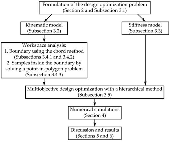
Figure 1. Organization of this paper.

2. Manipulator Design and Problem Formulation

Figure 2 shows a computer model and a prototype of the considered manipulator. Its main component is a planar parallel mechanism with four branches. Each branch includes cylinder 3 and piston 4, which form the actuated prismatic joint. The cylinders are attached to plate 2 with revolute joints, and the pistons are attached to platform 5 with revolute joints as well. The revolute joints on either side of platform 5 have collinear axes. The parallel mechanism provides platform 5 with three DOFs relative to plate 2: two translational DOFs along the $Oy$ and $Oz$ axes and one rotational DOF about the $Ox$ axis. Plate 2 is attached rigidly to two synchronously actuated carriages. These carriages translate the plate and the parallel mechanism relative to base 1 along the $Ox$ axis. Finally, end-effector 6 rotates relative to platform 5. Therefore, the manipulator and its end-effector have five DOFs, including three translational and two rotational DOFs.

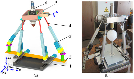
Figure 2. Considered manipulator: (a) computer model; (b) prototype during the operation.

The planar parallel mechanism has redundant actuation: four linear drives control the three DOFs of platform 5. This redundancy serves multiple purposes. First, it prevents singular configurations where the platform can gain uncontrolled DOFs. Second, it enhances the mechanism stiffness. Finally, the symmetrical design of the manipulator makes it more suitable for practical applications. Among them are additive technologies like selective laser sintering or 3D printing. For example, Figure 2a represents end-effector 6 as a laser beam unit.

Figure 2b shows the manipulator prototype. The end-effector imitates this laser beam unit and has similar weight and dimensions. The video in the Supplementary Materials demonstrates the prototype in action, with the end-effector tip tracing a curve on a sphere.

Our computer simulations and experiments showed that the manipulator was not stiff in the lateral direction (along the $Oy$ axis). The stiffness in this direction is determined by the stiffness of the parallel mechanism, whose geometrical parameters were not chosen correctly. Thus, it becomes necessary to perform the dimensional synthesis of the mechanism and identify these parameters, which is the main goal of this article. The following section explains the procedure for solving the synthesis problem in more detail.

3. Dimensional Synthesis

The dimensional synthesis of a mechanism involves computing the geometrical parameters of its links to optimize some performance metrics [11]. Section 3.1, Section 3.2, Section 3.3 discuss these parameters and metrics applied to the considered mechanism. Next, Section 3.4 introduces the methods of workspace analysis, which is a necessary step in solving the dimensional synthesis problem. Finally, Section 3.5 transforms this problem into a multi-objective optimization problem and presents an algorithm to solve it.

3.1. Geometrical Parameters

The primary goal of the dimensional synthesis considered in this paper is to choose manipulator geometrical parameters to increase its lateral stiffness. As stated in Section 2, this is the planar parallel mechanism whose parameters influence this stiffness. In this regard, the rest of our analysis focuses on this 3-DOF mechanism and ignores two remaining DOFs that do not affect the dimensional synthesis: translation along the $Ox$ axis and the end-effector rotation relative to the platform.

The geometrical parameters of the mechanism include the lengths of its links and the coordinates of the joint axes. We assume the platform dimensions and the stroke length of the linear drives are already specified from the preceding workspace analysis [26] and prototyping (Figure 2b). The only variable geometrical parameters are coordinates ${\mathbf{p}}_{Ai}$ of plate revolute joints $A_i$, $i=1,\dots ,4$ (Figure 3a). We consider the planar case, so each vector ${\mathbf{p}}_{Ai}$ has two unknown components—there are eight unknown parameters in total. Since the mechanism has a symmetrical design, we can reduce the number of these parameters to three. They include variables $y_1$ and $y_2$, which define the y coordinates of the joints, and variable h, which defines the z coordinate of the upper joint (Figure 3a).

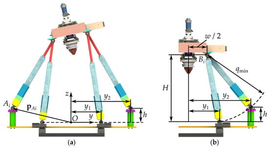
Figure 3. The parallel mechanism: (a) general configuration; (b) lowest configuration.

Furthermore, we can reduce the number of variables from three to two if we consider the following auxiliary condition. In the lowest configuration of the mechanism, each branch has a length of $q_{\min }$. Points $A_i$ of two adjacent branches belong to a circle with radius $q_{\min }$ centered at points $B_i$, the centers of the platform revolute joints, which coincide for these two branches (Figure 3b). We can use Pythagoras’ theorem to compute height H of point $B_i$ in the considered configuration as a function of variable $y_1$:

$$H=\sqrt{q_{\min }^2-{(y_1-w/2)}^2},$$

(1)

where w is a width of the platform, which is known from the mechanism design.

Now, we use Equation (1) and express variable h as a function of $y_1$ and $y_2$:

$$h=H-\sqrt{q_{\min }^2-{(y_2-w/2)}^2}.$$

(2)

Thus, we reduced the number of variables in the dimensional synthesis problem from eight components of vectors ${\mathbf{p}}_{Ai}$, $i=1,\dots ,4$, to two parameters, $y_1$ and $y_2$, defining the mechanism geometry. The synthesis problem in this paper involves determining these parameters considering stiffness criteria, whose model is established in Section 3.3. This model needs a Jacobian matrix of the mechanism, and the next subsection presents the required kinematic relations.

3.2. Kinematic Model

This subsection aims to derive kinematic relations, which are prerequisites for developing a stiffness model and solving the dimensional synthesis problem. The first task is to solve the inverse kinematic problem, i.e., to determine displacements in the mechanism joints for the specified posture of its end-effector. We can describe the latter by parameters y and z, which are the coordinates of end-effector tip C, and angle $\phi$, which determines the end-effector orientation (Figure 4). The joint displacements include stroke $q_i$ of the linear drive and angles ${\alpha }_i$ and ${\beta }_i$ in the passive revolute joints of the i-th branch, $i=1,\dots ,4$.

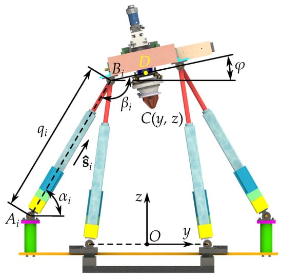
Figure 4. Kinematic parameters of the mechanism.

First, we can compute stroke $q_i$ from the equation that relates the coordinates of points $A_i$ and $B_i$:

$$q_i^2={({\mathbf{p}}_{Ai}-{\mathbf{p}}_{Bi})}^2,$$

(3)

where ${\mathbf{p}}_{Ai}$ and ${\mathbf{p}}_{Bi}$ are the position vectors of points $A_i$ and $B_i$ in base reference frame $Oyz$:

$${\mathbf{p}}_{A1}=\left[\begin{array}{c}-y_1\\ 0\end{array}\right],{\mathbf{p}}_{A2}=\left[\begin{array}{c}-y_2\\ h\end{array}\right],{\mathbf{p}}_{A3}=\left[\begin{array}{c}{y}_1\\ 0\end{array}\right],{\mathbf{p}}_{A4}=\left[\begin{array}{c}{y}_2\\ h\end{array}\right],$$

(4a)

$$\begin{array}{c}{\mathbf{p}}_{Bi}=\left[\begin{array}{c}y\\ z\end{array}\right]+{\mathbf{p}}_{CBi}=\left[\begin{array}{c}y\\ z\end{array}\right]+\left[\begin{array}{cc}cos\left(\phi \right)& -sin\left(\phi \right)\\ sin\left(\phi \right)& cos\left(\phi \right)\end{array}\right]{\mathbf{r}}_{CBi},\\ {\mathbf{r}}_{CB1}={\mathbf{r}}_{CB2}=\left[\begin{array}{c}{l}_{CD}\\ -w/2\end{array}\right],{\mathbf{r}}_{CB3}={\mathbf{r}}_{CB4}=\left[\begin{array}{c}{l}_{CD}\\ w/2\end{array}\right].\end{array}$$

(4b)

Coordinates ${\mathbf{p}}_{Ai}$ in Equation (4a) depend on the mechanism geometry, and we compute them according to Figure 3 and Equations (1) and (2). Coordinates ${\mathbf{p}}_{Bi}$ in Equation (4b) depend on the end-effector posture and parameters w and $l_{CD}$, which are the platform width and the distance between points C and D, respectively (Figure 4).

Let ${\widehat{\mathbf{s}}}_i$ be a unit vector parallel to line $A_i{B}_i$:

$${\widehat{\mathbf{s}}}_i={\displaystyle \frac{1}{q_i}}({\mathbf{p}}_{Bi}-{\mathbf{p}}_{Ai})=\left[\begin{array}{c}{s}_i^y\\ s_i^z\end{array}\right].$$

(5)

Now, we can determine the remaining angles in the passive revolute joints as follows:

$${\alpha }_i=atan2(s_i^z,s_i^y),{\beta }_i=\pi +\phi -{\alpha }_i,$$

(6)

where atan2 is the two-argument arctangent function [28] (ch. 6).

Thus, we expressed displacements in all joints of the mechanism in terms of the end-effector configuration, defined by parameters y, z, and $\phi$. The next step of the kinematic analysis is to derive the Jacobian matrix of the mechanism, which relates infinitesimal displacements $\delta q_i$, $i=1,\dots ,4$, in the actuated joints and infinitesimal displacements $\delta y$, $\delta z$, and $\delta \phi$ of the end-effector. For this purpose, we differentiate both sides of Equation (3). Considering Equation (5) and rearranging the terms, we obtain:

$$\delta q_i={\widehat{\mathbf{s}}}_i^{\mathrm{T}}\delta {\mathbf{p}}_{CBi}=\left[\begin{array}{cc}{\widehat{\mathbf{s}}}_i^{\mathrm{T}}& det\left(\left[\begin{array}{cc}{\mathbf{p}}_{CBi}& {\widehat{\mathbf{s}}}_i\end{array}\right]\right)\end{array}\right]\left[\begin{array}{c}\delta y\\ \delta z\\ \delta \phi \end{array}\right]={\mathbf{j}}_i^{\mathrm{T}}\delta \mathbf{p}.$$

(7)

Vector $\mathbf{p}$ in the equation above includes the end-effector coordinates, while vector ${\mathbf{j}}_i$ is a planar “version” of the Plücker coordinates of line $A_i{B}_i$, where the third component is a moment of this line about point C [29]. Combining Equations (7) for all branches, we obtain:

$$\delta \mathbf{q}=\mathbf{J}\delta \mathbf{p},$$

(8)

where $\mathbf{q}={\left[q_1{q}_2{q}_3{q}_4\right]}^{\mathrm{T}}$ is a vector of actuated coordinates; $\mathbf{J}={\left[{\mathbf{j}}_1{\mathbf{j}}_2{\mathbf{j}}_3{\mathbf{j}}_4\right]}^{\mathrm{T}}$ is the $4\times 3$ Jacobian matrix of the mechanism. The matrix is rectangular because of the redundant actuation. We  use this matrix in the stiffness model considered in the next subsection.

3.3. Stiffness Model

Scholars have proposed various models and measures to analyze the stiffness of parallel mechanisms [30]. The links of the considered mechanism are made of duraluminum, and we assume their stiffness dominates the stiffness of the drives. This is a typical assumption for stiffness modeling of planar parallel mechanisms [31]. Therefore, we apply a conventional stiffness model where the drives are the only source of compliance [32].

To derive the stiffness model, we consider a static configuration of the mechanism when its drives are locked. Our goal is to find a relation that connects the load exerted to the end-effector with its displacements caused by this load. Let $\mathbf{w}$ be a wrench applied at end-effector tip C. This wrench summarizes all possible external forces and torques acting on the end-effector. We can express it component-wise as $\mathbf{w}={\left[f_y{f}_z{\tau }_x\right]}^{\mathrm{T}}$, where $f_y$, $f_z$, and ${\tau }_x$ represent the forces along the $Oy$ and $Oz$ axes and the torque about the $Ox$ axis. When wrench $\mathbf{w}$ acts on the mechanism end-effector, the latter rotates by angle $\delta \phi$ about the $Ox$ axis, and its tip C displaces by $\delta y$ and $\delta z$ along the $Oy$ and $Oz$ axes. We can combine these displacements into vector $\delta \mathbf{p}={\left[\delta y\delta z\delta \phi \right]}^{\mathrm{T}}$. At the same time, the i-th drive of the mechanism, $i=1,\dots ,4$, generates torque ${\tau }_i$ proportional to stroke elongation $\delta q_i$:

$${\tau }_i=c\delta q_i,$$

(9)

where c is a drive stiffness, which we assume identical for each drive.

These torques must balance wrench $\mathbf{w}$, so we can write [32]:

$$\mathbf{w}={\mathbf{J}}^{\mathrm{T}}\mathbf{\tau },$$

(10)

where $\mathbf{\tau }={\left[{\tau }_1{\tau }_2{\tau }_3{\tau }_4\right]}^{\mathrm{T}}$ and $\mathbf{J}$ is the Jacobian matrix derived in the previous subsection. Combining Equations (8), (9), and (10), we obtain the desired expression:

$$\mathbf{w}=c{\mathbf{J}}^{\mathrm{T}}\mathbf{J}\delta \mathbf{p}=\mathbf{K}\delta \mathbf{p},$$

(11)

where $\mathbf{K}=c{\mathbf{J}}^{\mathrm{T}}\mathbf{J}$ is the stiffness matrix of the mechanism.

Finally, we can rewrite the obtained equation in a component-wise form:

$$\left[\begin{array}{c}{f}_y\\ f_z\\ {\tau }_x\end{array}\right]=\left[\begin{array}{ccc}{k}_y& \cdots & \cdots \\ \cdots & k_z& \cdots \\ \cdots & \cdots & k_{\phi }\end{array}\right]\left[\begin{array}{c}\delta y\\ \delta z\\ \delta \phi \end{array}\right],$$

(12)

where parameters $k_y$ and $k_z$ characterize the mechanism stiffness along the $Oy$ and $Oz$ axes, respectively; parameter $k_{\phi }$ characterizes the rotational stiffness of the mechanism about the $Ox$ axis; “⋯” indicate other components of stiffness matrix $\mathbf{K}$ that characterize the “cross-coupled” stiffness.

As discussed in Section 2, the dimensional synthesis problem considered in this paper aims to enhance the lateral stiffness of the mechanism. This is parameter $k_y$ that characterizes this stiffness. However, maximizing this parameter can decrease the mechanism stiffness in other directions, as well as its overall stiffness. In this regard, we consider two additional stiffness indices. The first one is parameter $k_z$ characterizing the vertical stiffness. The second one is the inverse condition number $k^{-1}=\sqrt{{\lambda }_{\min }/{\lambda }_{\max }}$ of stiffness matrix $\mathbf{K}$, characterizing the overall stiffness of the mechanism, where ${\lambda }_{\min }$ and ${\lambda }_{\max }$ are the minimum and maximum eigenvalues of matrix $\mathbf{K}$.

The reason that we consider the inverse condition number is because it varies between zero and one, which gives more representative results. The closer its value is to zero, the lower the mechanism stiffness, and vice versa. One should note from Equation (7) that Jacobian matrix $\mathbf{J}$ is nonhomogeneous in units. Therefore, stiffness matrix $\mathbf{K}$ is nonhomogeneous in units too. This nonhomogeneity can lead to incorrect results when computing parameter $k^{-1}$. To overcome this issue, we use a standard trick and normalize the last column of Jacobian matrix $\mathbf{J}$ by a characteristic length [11] (ch. 2), which we set equal to the length of $C{B}_i$. Thus, we compute the inverse condition number $k^{-1}$ for normalized stiffness matrix ${\mathbf{K}}_{\mathrm{n}}=c{\mathbf{J}}_{\mathrm{n}}^{\mathrm{T}}{\mathbf{J}}_{\mathrm{n}}$, where ${\mathbf{J}}_{\mathrm{n}}$ is the normalized Jacobian matrix whose rows ${\mathbf{j}}_{\mathrm{n}i}^{\mathrm{T}}$, $i=1,\dots ,4$, have the following representation:

$${\mathbf{j}}_{\mathrm{n}i}^{\mathrm{T}}=\left[\begin{array}{cc}{\widehat{\mathbf{s}}}_i^{\mathrm{T}}& {\displaystyle \frac{det\left(\left[\begin{array}{cc}{\mathbf{p}}_{CBi}& {\widehat{\mathbf{s}}}_i\end{array}\right]\right)}{\parallel {\mathbf{p}}_{CBi}\parallel }}\end{array}\right].$$

(13)

Normalization of Jacobian matrix $\mathbf{J}$ does not affect indices $k_y$ and $k_z$, and they can be computed using either matrix $\mathbf{K}$ or normalized matrix ${\mathbf{K}}_{\mathrm{n}}$. Since the Jacobian matrix depends on the mechanism posture, indices $k_y$, $k_z$, and $k^{-1}$ depend on this posture too. To estimate the mechanism stiffness, we compute the average values of these indices over the mechanism workspace:

$${\overline{k}}_y={\displaystyle \frac{{\int }_W{k}_y\mathrm{d}W}{W}},{\overline{k}}_z={\displaystyle \frac{{\int }_W{k}_z\mathrm{d}W}{W}},{\overline{k}}^{-1}={\displaystyle \frac{{\int }_W{k}^{-1}\mathrm{d}W}{W}},$$

(14)

where W is the workspace area.

In practice, it is usually difficult to evaluate the integrals in Equation (14). The standard way to overcome this issue is to sample the workspace and take the average values of the stiffness indices evaluated in the discrete points [11] (ch. 1). The denser the discrete points, the more accurate results we obtain. The following subsection presents the algorithm to determine the mechanism workspace and perform this sampling.

3.4. Workspace Analysis

Solving the dimensional synthesis problem requires computing the mechanism workspace for various combinations of geometrical parameters $y_1$ and $y_2$ and evaluating indices ${\overline{k}}_y$, ${\overline{k}}_z$, and ${\overline{k}}^{-1}$ over the obtained workspace. Since the mechanism end-effector has three DOFs (two translational and one rotational), there are several types of workspaces [30]. In this paper, we focus on translation workspaces—the set of the end-effector postures (coordinates y and z) where it has fixed orientation (fixed angle $\phi$).

The standard approach to determine the workspace in dimensional synthesis problems is to sample the coordinate space around the end-effector, solve the inverse kinematics for each sampled point, and check the joint constraints. For the considered mechanism, we can express these constraints by the following conditions:

$$q_{\min }\le q_i\le q_{\max },{\alpha }_{\min }\le {\alpha }_i\le {\alpha }_{\max },{\beta }_{\min }\le {\beta }_i\le {\beta }_{\max },i=1,\dots ,4,$$

(15)

where “min” and “max” mean the minimum and maximum values of the corresponding joint displacements, which we assume to be identical for each branch.

Thus, the workspace analysis involves sampling the $y-z$ coordinate space, applying Equations (3)–(6) derived in Section 3.2, and checking conditions in Equation (15). We need to repeat this procedure for each combination of parameters $y_1$ and $y_2$. This can be computationally expensive, because the accurate results need dense sampling, increasing the computation time.

In this regard, we propose an alternative approach for the workspace analysis. First, we use the chord method [26,33] to find the workspace boundary, and then we sample the workspace inside the obtained boundary. The chord method is an optimization-based computationally effective tool, which allows determining the boundary of nonconvex workspaces as well. The subsequent paragraphs outline the applied techniques.

3.4.1. Finding a Point on the Boundary

The initial step in computing the workspace is to find a boundary point. First, we select point $U_0$ for which we know it will be inside the workspace (Figure 5). This choice is often self-evident, and we can set coordinates ${\mathbf{u}}_0$ of point $U_0$ to be approximately near the expected workspace center:

$${\mathbf{u}}_0=\left[\begin{array}{c}0\\ (q_{\min }+q_{\max })/2-l_{CD}\end{array}\right].$$

(16)

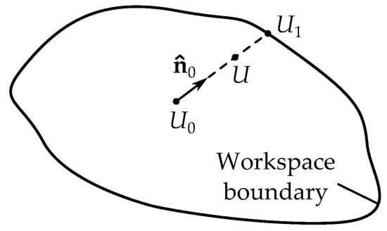
Figure 5. Determining the starting point on the workspace boundary.

After that, we consider a ray starting from point $U_0$ in a direction defined by unit vector ${\widehat{\mathbf{n}}}_0$ (Figure 5). Let U be a point on this ray with coordinates $\mathbf{u}={\left[yz\right]}^{\mathrm{T}}$. If we “move” point U along the ray, the first point for which a solution to the inverse kinematic problem violates any joint constraint will be the boundary point. We can define the corresponding optimization problem that computes the coordinates of this point:

$$\begin{array}{ccc}\hfill \underset{\mathbf{u}}{max}& \parallel \mathbf{u}-{\mathbf{u}}_0\parallel ,\hfill & \\ \hfill \mathrm{s}.\mathrm{t}.& q_{\min }\le q_i\left(\mathbf{u}\right)\le q_{\max },\hfill & \hfill i=1,\dots ,4,\\ \hfill & {\alpha }_{\min }\le {\alpha }_i\left(\mathbf{u}\right)\le {\alpha }_{\max },\hfill & \hfill i=1,\dots ,4,\\ \hfill & {\beta }_{\min }\le {\beta }_i\left(\mathbf{u}\right)\le {\beta }_{\max },\hfill & \hfill i=1,\dots ,4,\\ \hfill & y_{\min }\le y\le y_{\max },\hfill & \\ \hfill & {(\mathbf{u}-{\mathbf{u}}_0)}^{\mathrm{T}}{\widehat{\mathbf{n}}}_0=\parallel \mathbf{u}-{\mathbf{u}}_0\parallel .\hfill \end{array}$$

(17)

In the optimization problem above, we omit angle $\phi$, because we consider it to be predefined for this problem. We compute joint displacements $q_i$, ${\alpha }_i$, and ${\beta }_i$ using the inverse kinematics and Equations (3)–(6). Inequality $y_{\min }\le y\le y_{\max }$ is an auxiliary condition that limits the workspace width and comes from practical considerations. The last equality condition in problem (17) ensures that point U remains on the ray.

To solve this problem, we define the initial guess as ${\mathbf{u}}_0+{\delta }_0{\widehat{\mathbf{n}}}_0$, where ${\delta }_0$ is a small step along the ray. A solution to the optimization problem gives us coordinates ${\mathbf{u}}_1$ of point $U_1$ that belongs to the workspace boundary. It is the starting point for constructing the whole boundary using the chord method, as discussed further.

3.4.2. Tracing the Boundary

Starting at point $U_1$, we determine other points $U_2,U_3,\dots$ on the boundary by successive circular searches with constant chord length d. For example, let $U_j$ be a boundary point with coordinates ${\mathbf{u}}_j$ and ${\widehat{\mathbf{n}}}_j$ be a unit vector directed outside the workspace (Figure 6a). We consider arbitrary point U with coordinates $\mathbf{u}={\left[yz\right]}^{\mathrm{T}}$, which stays on a circle with radius d centered at point $U_j$. Vector ${\mathbf{t}}_j=\mathbf{u}-{\mathbf{u}}_j$ directs from $U_j$ to U and forms angle $\psi$ with vector ${\widehat{\mathbf{n}}}_j$:

$$\psi =\left\{\begin{array}{cc}acos\left({\displaystyle \frac{{\widehat{\mathbf{n}}}_j^{\mathrm{T}}{\mathbf{t}}_j}{\parallel {\mathbf{t}}_j\parallel }}\right),\hfill & \mathrm{if}\sigma \ge 0,\hfill \\ 2\pi -acos\left({\displaystyle \frac{{\widehat{\mathbf{n}}}_j^{\mathrm{T}}{\mathbf{t}}_j}{\parallel {\mathbf{t}}_j\parallel }}\right),\hfill & \mathrm{if}\sigma <0,\hfill \end{array}\right.$$

(18)

where $\sigma =n_j^y{t}_j^z-n_j^z{t}_j^y$, with $n_j^y$, $n_j^z$, $t_j^y$, and $t_j^z$ being the corresponding components of vectors ${\widehat{\mathbf{n}}}_j$ and ${\mathbf{t}}_j$. Parameter $\sigma$ is used to select the angle between these vectors in a counter-clockwise direction (Figure 6b).

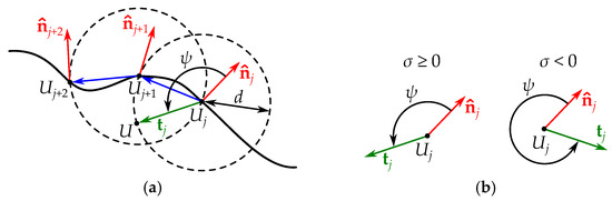
Figure 6. Computing the workspace boundary using the chord method: (a) finding point $U_{j+1}$ by a circular search at point $U_j$; (b) angle $\psi$ depending on the $\sigma$ value.

To find the next point on the workspace boundary (point $U_{j+1}$), we “move” point U along the circle and solve the inverse kinematic problem for coordinates $\mathbf{u}$ until any joint constraint is violated, which indicates that we have found the boundary point. This procedure is equivalent to minimizing angle $\psi$, and it corresponds to the following optimization problem:

$$\begin{array}{ccc}\hfill \underset{\mathbf{u}}{min}& \psi ,\hfill & \\ \hfill \mathrm{s}.\mathrm{t}.& q_{\min }\le q_i\left(\mathbf{u}\right)\le q_{\max },\hfill & \hfill i=1,\dots ,4,\\ \hfill & {\alpha }_{\min }\le {\alpha }_i\left(\mathbf{u}\right)\le {\alpha }_{\max },\hfill & \hfill i=1,\dots ,4,\\ \hfill & {\beta }_{\min }\le {\beta }_i\left(\mathbf{u}\right)\le {\beta }_{\max },\hfill & \hfill i=1,\dots ,4,\\ \hfill & y_{\min }\le y\le y_{\max },\hfill & \\ \hfill & {(\mathbf{u}-{\mathbf{u}}_j)}^2=d^2.\hfill \end{array}$$

(19)

The last equality condition in the optimization problem above ensures that point $U_j$ belongs to the circle. We define the initial guess as ${\mathbf{u}}_j-\delta {\widehat{\mathbf{n}}}_j$, where $\delta$ is a small step “inside” the workspace. A solution to this problem gives us coordinates ${\mathbf{u}}_{j+1}$ of point $U_{j+1}$. We can now compute ${\mathbf{t}}_j={\mathbf{u}}_{j+1}-{\mathbf{u}}_j$ (the blue arrows in Figure 6a) and define unit vector ${\widehat{\mathbf{n}}}_{j+1}$ for the next circular search:

$${\widehat{\mathbf{n}}}_{j+1}=\left[\begin{array}{c}cos(atan2(t_j^z,t_j^y)-\pi /2)\\ sin(atan2(t_j^z,t_j^y)-\pi /2)\end{array}\right].$$

(20)

We solve optimization problems (19) consecutively for $j=1,2,\dots$, starting with point $U_1$ and vectors ${\widehat{\mathbf{n}}}_1={\widehat{\mathbf{n}}}_0$ and ${\mathbf{u}}_1$, obtained after solving problem (17). The algorithm terminates with point $U_n$ when the following conditions are satisfied:

$$\parallel {\mathbf{u}}_n-{\mathbf{u}}_1\parallel \le d\mathrm{and}\parallel {\mathbf{u}}_n-{\mathbf{u}}_2\parallel \le d.$$

(21)

As a result, we have a set of coordinates ${\mathbf{u}}_1,\dots ,{\mathbf{u}}_n$ of n points $U_1,\dots ,U_n$ that define the workspace boundary. The smaller chord length d, the more precise boundary we get. Article [33] discusses other issues of the chord method in more detail. Now, we can sample the workspace inside the boundary using the method discussed next.

3.4.3. Sampling Inside the Boundary

To sample the workspace inside the obtained boundary, we first determine the rectangle that envelops this boundary. Let $V_1{V}_2{V}_3{V}_4$ be this rectangle, whose vertices have coordinates ${\mathbf{v}}_1,\dots ,{\mathbf{v}}_4$ (Figure 7). We compute these coordinates as follows:

$${\mathbf{v}}_1=\left[\begin{array}{c}\underset{j}{min}\left(y_j\right)\\ \underset{j}{min}\left(z_j\right)\end{array}\right],{\mathbf{v}}_2=\left[\begin{array}{c}\underset{j}{max}\left(y_j\right)\\ \underset{j}{min}\left(z_j\right)\end{array}\right],{\mathbf{v}}_3=\left[\begin{array}{c}\underset{j}{max}\left(y_j\right)\\ \underset{j}{max}\left(z_j\right)\end{array}\right],{\mathbf{v}}_4=\left[\begin{array}{c}\underset{j}{min}\left(y_j\right)\\ \underset{j}{max}\left(z_j\right)\end{array}\right],$$

(22)

where $y_j$ and $z_j$ are the corresponding components of vector ${\mathbf{u}}_j$, $j=1,\dots ,n$.

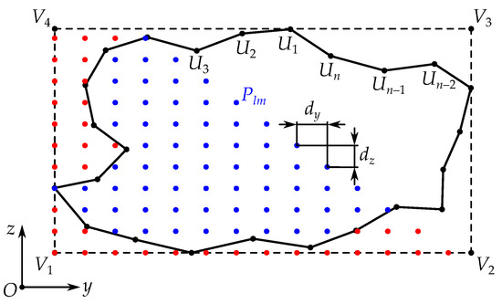
Figure 7. Sampling rectangle $V_1{V}_2{V}_3{V}_4$ that envelops workspace boundary $U_1{U}_2\dots U_n$. The blue and red dots are examples of samples inside and outside the boundary.

After that, we sample the $Oyz$ plane inside the rectangle. Let $d_y$ and $d_z$ be the sample steps along the $Oy$ and $Oz$ axes (Figure 7). We determine numbers $n_y$ and $n_z$ of samples along these axes using the following expressions:

$$n_y=⌈{\displaystyle \frac{v_2^y-v_1^y}{d_y}}⌉,n_z=⌈{\displaystyle \frac{v_3^z-v_2^z}{d_z}}⌉,$$

(23)

where $v_1^y$, $v_2^y$, $v_2^z$, and $v_3^z$ are the corresponding components of vectors ${\mathbf{v}}_1$, ${\mathbf{v}}_2$, and ${\mathbf{v}}_3$; $\lceil \dots \rceil$ is the ceiling function that gives the lowest integer greater or equal to its argument.

Thus, we sampled rectangle $V_1{V}_2{V}_3{V}_4$ into points $P_{lm}$ with coordinates ${\mathbf{p}}_{lm}$:

$${\mathbf{p}}_{lm}={\mathbf{v}}_1+\left[\begin{array}{c}(l-1)d_y\\ (m-1)d_z\end{array}\right],l=1,\dots ,n_y,m=1,\dots ,n_z.$$

(24)

The next step is to check which sample points stay inside the workspace boundary, i.e., which points are inside polygon $U_1{U}_2\dots U_n$. For this purpose, we follow the procedure proposed by Hormann and Agathos [34], whose details are outlined below.

Let $P_{lm}$ be a point under consideration. This point defines four quadrants in the $Oyz$ plane, as shown in Figure 8a. For each polygon vertex (boundary point) $U_j$, $j=1,\dots ,n$, we assign number $a_j\in \{0,1,2,3\}$, whose value depends on the quadrant of point $U_j$. Next, for each polygon edge $U_j{U}_{j+1}$, we compute number $b_j=a_{j+1}-a_j$ (for $j=n$, we consider edge $U_n{U}_1$ and compute $b_n=a_1-a_n$). Finally, we calculate number $\omega$ using Algorithm 1.

Algorithm 1: Computing number $\omega$ to check if point $P_{lm}$ is in polygon $U_1\dots U_n$.

where

$$f\left(j\right)=det\left(\left[\begin{array}{cc}{\mathbf{u}}_j-{\mathbf{p}}_{lm}& {\mathbf{u}}_{j+1}-{\mathbf{p}}_{lm}\end{array}\right]\right).$$

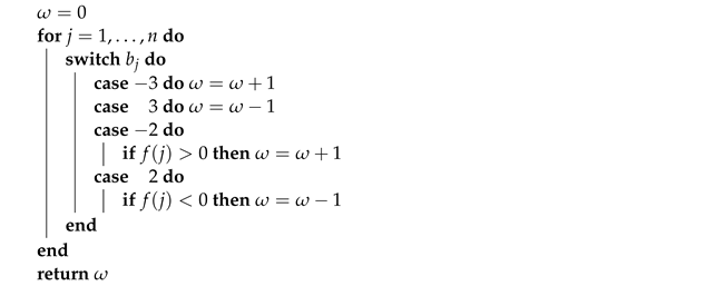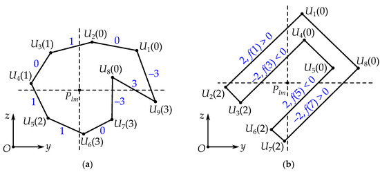
Figure 8. Numbering of polygon vertices and edges: (a) the numbers near the vertices inside the parentheses correspond to values $a_j$, while the blue numbers near the edges are values $b_j$; (b) edge $U_1{U}_2$ with $b_1=2$ and $f\left(1\right)>0$ and edge $U_3{U}_4$ with $b_3=-2$ and $f\left(3\right)<0$ are not counted in Algorithm 1, as they do not match the if statements of the algorithm.

Algorithm 1 actually determines how many times the ray starting at point $P_{lm}$ and directing along the $Oy$ axis intersects the polygon edges, considering the “direction” of these edges. The resulting value of number $\omega$ can be either 0 or 1. If $\omega =1$, point $P_{lm}$ is inside the polygon, i.e., inside the workspace boundary. Function $f\left(j\right)$, applied to vertices $U_j$ and $U_{j+1}$ in opposite quadrants, checks the orientation of triangle $P_{lm}{U}_j{U}_{j+1}$ and excludes the edges that do not intersect the ray (Figure 8b).

Note that Algorithm 1 includes only summation, subtraction, and multiplication operations, and it is suitable for nonconvex polygons as well. Therefore, we can determine which workspace samples are inside the boundary in a computationally effective manner. It allows us to set sample steps $d_y$ and $d_z$ smaller than chord length d and obtain a dense sampling, which improves the accuracy of results.

As a result, we have a set of N points with coordinates ${\mathbf{p}}_1,\dots ,{\mathbf{p}}_N$ that belong to the workspace. These are the points for which we compute the stiffness indices considered in Section 3.3. For this purpose, we use the following discrete representation of Equation (14):

$${\overline{k}}_y={\displaystyle \frac{{\sum }_{s=1}^N{k}_y\left({\mathbf{p}}_s\right)}{N}},{\overline{k}}_z={\displaystyle \frac{{\sum }_{s=1}^N{k}_z\left({\mathbf{p}}_s\right)}{N}},{\overline{k}}^{-1}={\displaystyle \frac{{\sum }_{s=1}^N{k}^{-1}\left({\mathbf{p}}_s\right)}{N}}.$$

(25)

3.5. Synthesis Algorithm

The methods discussed in Section 3.2, Section 3.3, Section 3.4 allow us to compute stiffness indices ${\overline{k}}_y$, ${\overline{k}}_z$, and ${\overline{k}}^{-1}$ for the given values of design parameters $y_1$ and $y_2$. In the dimensional synthesis, we specify ranges $y_{1\min }\le y_1\le y_{1\max }$ and $y_{2\min }\le y_2\le y_{2\max }$ for these parameters, sample the ranges with steps $d_{y1}$ and $d_{y2}$, and evaluate the indices for each sample. Because the mechanism has a symmetrical design, it suffices to consider the samples with $y_1\le y_2$. As a result, we obtain three sets of the stiffness indices: $\left\{{\overline{k}}_{yp}\right\}$, $\left\{{\overline{k}}_{zp}\right\}$, and $\left\{{\overline{k}}_p^{-1}\right\}$, $p=1,\dots ,K$, where K is a number of samples. Each sample p corresponds to a unique combination of parameters $y_1$ and $y_2$.

According to Section 2, our task is to maximize the lateral stiffness of the mechanism. A straightforward solution here is to choose a combination of parameters $y_1$ and $y_2$ corresponding to the largest element of set $\left\{{\overline{k}}_{yp}\right\}$. However, for this combination, the vertical and overall stiffness can diminish to unacceptable levels. Thus, we have a (discrete unconstrained) multi-objective optimization problem with conflicting stiffness criteria.

Scholars have proposed various methods to solve these problems [35,36]. In this work, we use a hierarchical ($\epsilon$-constraint) method, as discussed in [37]. It solves the challenge of finding the optimal solution on the Pareto frontier and provides a unique solution that meets designer preferences. Compared with another familiar approach of multi-objective optimization, the weighting sum method, it does not need to normalize objective functions and does not result in “corner” solutions, which are often impractical [37].

The hierarchical method proceeds as follows. First, we define four objective functions $f_1\left(p\right),\dots ,f_4\left(p\right)$ to be maximized in the following priority order:

$$\begin{array}{cccccccc}\hfill f_1:\mathcal{P}& \to \left\{{\overline{k}}_{yp}\right\},\hfill & \hfill f_2:\mathcal{P}& \to \left\{{\overline{k}}_p^{-1}\right\},\hfill & \hfill f_3:\mathcal{P}& \to \left\{{\overline{k}}_{zp}\right\},\hfill & \hfill f_4:\mathcal{P}& \to \left\{W_p\right\},\hfill \\ \hfill p& \mapsto {\overline{k}}_{yp},\hfill & \hfill p& \mapsto {\overline{k}}_p^{-1},\hfill & \hfill p& \mapsto {\overline{k}}_{zp},\hfill & \hfill p& \mapsto W_p,\hfill \end{array}$$

(26)

where $\mathcal{P}=\{1,\dots ,K\}$ is a set of sample numbers; $\left\{W_p\right\}$ is a set of workspace areas $W_1,\dots$, $W_K$, which we can compute approximately using the next equation:

$$W_p\approx N_p{d}_y{d}_z,$$

(27)

where $N_p$ is a number of points inside the workspace boundary for the p-th combination of parameters $y_1$ and $y_2$.

We include the fourth objective function in Equation (26) because the workspace shape and dimensions change as we vary parameters $y_1$ and $y_2$. Function $f_1\left(p\right)$, which evaluates the lateral stiffness, has the highest priority according to a specified task. Function $f_2\left(p\right)$, which evaluates the overall stiffness, has the second priority in this paper.

After that, the hierarchical optimization follows the next steps [37]:

1.

Find the maximum and minimum values of each objective function over set $\mathcal{P}$:

$$f_i^{\max }=\underset{p\in \mathcal{P}}{max}{f}_i\left(p\right),f_i^{\min }=\underset{p\in \mathcal{P}}{min}{f}_i\left(p\right),i=1,\dots ,4.$$

(28)

Considering Equation (26), we can compute these values in a straightforward manner.

2.

Solve the following optimization problems sequentially for $i=2,3,4$:

$$\begin{array}{ccc}\hfill \underset{p}{max}& f_i\left(p\right),\hfill & \\ \hfill \mathrm{s}.\mathrm{t}.& p\in \mathcal{P},\hfill & \\ \hfill & f_r\left(p\right)\ge f_r^{*}-{\epsilon }_r(f_r^{*}-f_r^{\min }),\hfill & \hfill r=1,\dots ,i-1,\end{array}$$

(29)

where $f_r^{*}$ is the optimal value of the $f_r$ objective function after solving the r-th optimization problem, and we have $f_1^{*}=f_1^{\max }$; ${\epsilon }_r$ is used to set a “distance” to optimum value $f_r^{*}$. Similar to problems (28), we can solve each optimization problem by simple evaluation of the objective functions over set $\mathcal{P}$.

The hierarchical procedure above relies on the following idea. First, we solve the optimization problem for the most important objective function. Next, we consider the less important objectives, and parameter ${\epsilon }_r$ indicates what portion of the already optimized objective we can sacrifice when optimizing the next objective. A solution to the last ($i=4$) optimization problem (29) corresponds to the optimal values of parameters $y_1$ and $y_2$.

A major challenge in this approach is to choose the values of parameters ${\epsilon }_r$, $r=1,2,3$. This choice depends on the importance of the r-th objective function $f_r$ and its potential conflicts with other objectives. Following the techniques from [37], we introduce a metric to measure the conflict between the objectives. Let $p_i^{*}={argmax}_{p\in \mathcal{P}}{f}_i\left(p\right)$ be a solution to the i-th maximization problem in Equation (28), $i=1,\dots ,4$. Solution $p_i^{*}$ corresponds to vector ${\mathbf{y}}_i^{*}={\left[y_{1i}^{*}{y}_{2i}^{*}\right]}^{\mathrm{T}}$ of optimal design parameters $y_1$ and $y_2$. First, we compute “central” solution ${\mathbf{y}}_{\mathrm{c}}$ as the mean of these vectors:

$${\mathbf{y}}_{\mathrm{c}}={\displaystyle \frac{1}{4}}\sum _{i=1}^4{\mathbf{y}}_i^{*}.$$

(30)

Vector ${\mathbf{y}}_{\mathrm{c}}$ in the equation above approximates the center of the set of solutions. Next, we measure angle ${\theta }_{ij}$ between vectors ${\mathbf{y}}_i^{*}-{\mathbf{y}}_{\mathrm{c}}$ and ${\mathbf{y}}_j^{*}-{\mathbf{y}}_{\mathrm{c}}$, $i=1,\dots ,4$, $j=1,\dots ,4$:

$$cos\left({\theta }_{ij}\right)={\displaystyle \frac{{({\mathbf{y}}_i^{*}-{\mathbf{y}}_{\mathrm{c}})}^{\mathrm{T}}({\mathbf{y}}_j^{*}-{\mathbf{y}}_{\mathrm{c}})}{\parallel {\mathbf{y}}_i^{*}-{\mathbf{y}}_{\mathrm{c}}\parallel \parallel {\mathbf{y}}_j^{*}-{\mathbf{y}}_{\mathrm{c}}\parallel }},$$

(31)

and compute conflict indicator $c_{ij}$ between the i-th and j-th objective functions:

$$c_{ij}={\displaystyle \frac{1}{2}}\left(1-cos\left({\theta }_{ij}\right)\right).$$

(32)

The value of conflict indicator $c_{ij}$ varies between zero and one. The larger this value, the more conflicting the i-th and j-th objectives, while $c_{ij}=0$ means these objectives do not conflict; $c_{ii}$ is always equal to zero.

Finally, we define parameters ${\epsilon }_r$, $r=1,2,3$, using the expression below:

$${\epsilon }_r=\gamma \sum _{i=1}^4{c}_{ri}{w}_i,$$

(33)

where $w_i$ is a priority factor of the i-th objective function, such that ${\sum }_{i=1}^4{w}_i=1$; $\gamma$ is a scalar factor determined by numerical tests.

The weighted sum in Equation (33) has the following meaning. If high-priority objectives conflict with the r-th objective, we do not impose strict constraints on $f_r$ because it will restrict these high-priority objectives; thus, we obtain the big value of ${\epsilon }_r$. If the objectives conflicting with the r-th objective all have low priorities, it is not necessary to set strict constraints on $f_r$; the value of ${\epsilon }_r$ will be small.

This concludes the dimensional synthesis problem of the considered mechanism. We can summarize the entire synthesis procedure as a sequence of steps:

1.

Define constant parameters:

• Geometrical parameters of the manipulator: w, $l_{CD}$.
• Joint constraints: $q_{\min }$, $q_{\max }$, ${\alpha }_{\min }$, ${\alpha }_{\max }$, ${\beta }_{\min }$, ${\beta }_{\max }$.
• Drive stiffness: c.
• Parameters of the chord method: $y_{\min }$, $y_{\max }$, ${\widehat{\mathbf{n}}}_0$, ${\delta }_0$, $\delta$, d.
• Parameters of the workspace sampling method: $d_y$, $d_z$.
• Parameters of the design space sampling: $y_{1\min }$, $y_{1\max }$, $y_{2\min }$, $y_{2\max }$, $d_{y1}$, $d_{y2}$.
• Parameters of the hierarchical optimization: $\gamma$, $w_1,\dots ,w_4$.

2.

Define orientation $\phi$ of the end-effector.

3.

Sample parameters $y_1$ and $y_2$ (with $y_1\le y_2$) and determine number K of the samples.

4.

Perform the following for each sample $p=1,\dots ,K$:

• Find the first point on the workspace boundary by solving optimization problem (17).
• Find the whole boundary by solving a sequence of optimization problems (19).
• Sample the rectangle around the obtained boundary using Equations (22)–(24).
• Find $N_p$ sample points inside the rectangle using Algorithm 1.
• For each sample $s=1,\dots ,N_p$, determine the normalized stiffness matrix and compute the stiffness indices using Equations (11)–(13).
• Compute the average values of these stiffness indices using Equation (25).
• Compute the workspace area using Equation (27).

5.

Define objective functions $f_1,\dots ,f_4$ according to Equation (26) and find their maximum and minimum values by solving problems (28).

6.

Determine parameters ${\epsilon }_1$, ${\epsilon }_2$, and ${\epsilon }_3$ using Equations (30)–(33).

7.

Find the optimal values of design parameters $y_1$ and $y_2$ by solving a sequence of optimization problems (29).

The next section illustrates the proposed techniques with numerical examples.

4. Simulations and Results

Table 1 lists the geometrical parameters and joint constraints of the mechanism, which correspond to its computer model and prototype (Figure 2). Design parameters $y_1$ and $y_2$ were sampled within bounds $y_{1\min }=y_{2\min }=255\mathrm{mm}$ and $y_{1\max }=y_{2\max }=595\mathrm{mm}$ with steps $d_{y1}=d_{y2}=10\mathrm{mm}$. Considering condition $y_1\le y_2$, we obtained $K=630$ samples.

Table 1. Geometrical parameters and joint constraints of the considered mechanism ($i=1,\dots ,4$).

Parameter	Value
Platform width, w	298 mm
End-effector length, $l_{CD}$	163 mm
Minimum actuator stroke, $q_{\min }$	541 mm
Maximum actuator stroke, $q_{\max }$	841 mm
Minimum angle in joint $A_i$, ${\alpha }_{\min }$	${25}^{\circ }$
Maximum angle in joint $A_i$, ${\alpha }_{\max }$	${155}^{\circ }$
Minimum angle in joint $B_i$, ${\beta }_{\min }$	$7^{\circ }$
Maximum angle in joint $B_i$, ${\beta }_{\max }$	${173}^{\circ }$

Next, we determined the mechanism workspace and computed the stiffness indices for various orientations of the end-effector: angle $\phi$ was sampled in a range from $0^{\circ }$ to ${30}^{\circ }$ with a step of $5^{\circ }$ (we ignored the negative values because of the symmetrical design of the mechanism). As an example, Figure 9 illustrates the workspace boundary for various orientations with $y_1=255\mathrm{mm}$ and $y_2=505\mathrm{mm}$. We computed the boundary using the chord method with chord length $d=40\mathrm{mm}$ and other parameters specified in Table 2. Optimization problems (17) and (19) were solved in MATLAB using the standard function “fmincon” with its default settings. The figure shows the workspace diminishes as angle $\phi$ increases. The right vertical boundary of each workspace corresponds to right limit $y_{\max }=200\mathrm{mm}$ (Table 2), which was set for the chord method.

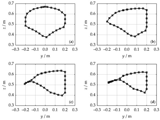
Figure 9. Workspace boundary for various end-effector orientations ($y_1=255\mathrm{mm}$, $y_2=505\mathrm{mm}$): (a) $\phi =0^{\circ }$; (b) $\phi ={10}^{\circ }$; (c) $\phi ={20}^{\circ }$; (d) $\phi ={30}^{\circ }$. The squares correspond to the boundary points.

Table 2. Parameters of the chord method for workspace analysis.

Parameter	Value
Chord length, d	40 mm
Left limit of the workspace, $y_{\min }$	$-200$ mm
Right limit of the workspace, $y_{\max }$	200 mm
Direction for the ray search, ${\widehat{\mathbf{n}}}_0$	${\left[01\right]}^{\mathrm{T}}$
Step for the initial guess in the ray search, ${\delta }_0$	10 mm
Step for the initial guess in the circular searches, $\delta$	10 mm

After that, we sampled the workspaces inside the obtained boundaries with sample steps $d_y=d_z=10\mathrm{mm}$, four times smaller than chord length d. Figure 10 shows the sampling results for $\phi =0^{\circ }$ and various values of design parameters $y_1$ and $y_2$, which were obtained using Algorithm 1. The workspaces not only have different shapes but are also slightly displaced along the $Oz$ axis. This concludes the workspace analysis of the mechanism. Without loss of generality, we exemplify subsequent results with these workspaces.

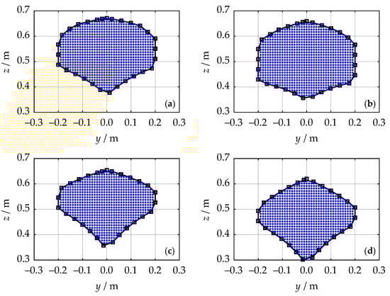
Figure 10. Workspace sampling for various parameters ($\phi =0^{\circ }$): (a) $y_1=255\mathrm{mm}$, $y_2=505\mathrm{mm}$; (b) $y_1=325\mathrm{mm}$, $y_2=425\mathrm{mm}$; (c) $y_1=345\mathrm{mm}$, $y_2=575\mathrm{mm}$; (d) $y_1=455\mathrm{mm}$, $y_2=575\mathrm{mm}$.

The next step was to determine stiffness maps, i.e., the distributions of stiffness indices $k_y$, $k_z$, and $k^{-1}$ over the obtained workspaces. Figure 11, Figure 12 and Figure 13 show these distributions over the workspaces from Figure 10. We defined drive stiffness $c=1\mathrm{N}/\mathrm{m}$ since it is just a scaling factor in Equation (11). In this regard, the values of the stiffness indices in Figure 11, Figure 12 and Figure 13 have no physical meaning, and we omit their units. Nonetheless, the stiffness maps allow us to estimate the regions of high and low stiffness and how they vary in percent.

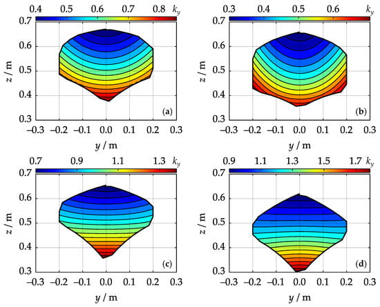
Figure 11. Stiffness maps of $k_y$ for various parameters ($\phi =0^{\circ }$): (a) $y_1=255\mathrm{mm}$, $y_2=505\mathrm{mm}$; (b) $y_1=325\mathrm{mm}$, $y_2=425\mathrm{mm}$; (c) $y_1=345\mathrm{mm}$, $y_2=575\mathrm{mm}$; (d) $y_1=455\mathrm{mm}$, $y_2=575\mathrm{mm}$.

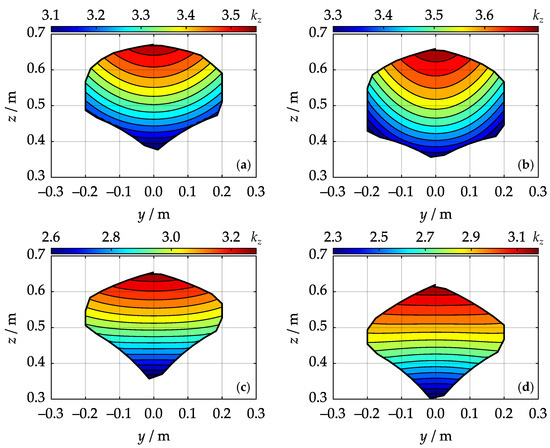
Figure 12. Stiffness maps of $k_z$ for various parameters ($\phi =0^{\circ }$): (a) $y_1=255\mathrm{mm}$, $y_2=505\mathrm{mm}$; (b) $y_1=325\mathrm{mm}$, $y_2=425\mathrm{mm}$; (c) $y_1=345\mathrm{mm}$, $y_2=575\mathrm{mm}$; (d) $y_1=455\mathrm{mm}$, $y_2=575\mathrm{mm}$.

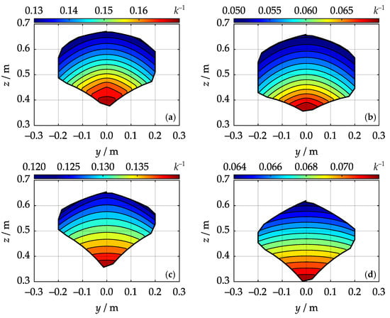
Figure 13. Stiffness map of $k^{-1}$ for various parameters ($\phi =0^{\circ }$): (a) $y_1=255\mathrm{mm}$, $y_2=505\mathrm{mm}$; (b) $y_1=325\mathrm{mm}$, $y_2=425\mathrm{mm}$; (c) $y_1=345\mathrm{mm}$, $y_2=575\mathrm{mm}$; (d) $y_1=455\mathrm{mm}$, $y_2=575\mathrm{mm}$.

Figure 11 indicates that the lateral stiffness is almost two times higher at the bottom of the workspace than at its top. This result is quite reasonable: in the uppermost configurations, the branches of the mechanism stay close to the vertical state, which lowers their ability to withstand lateral forces. If we compare Figure 11d with Figure 11b, we can see that the minimum value of $k_y$ increased three times (from 0.3 to 0.9). This is also an expected result: the “wider” the branches, the better they withstand lateral forces.

For similar reasons, the vertical stiffness of the mechanism is higher at the top of the workspace, and it decreases as the branches have wider placements (Figure 12). Thus, the indices of the lateral and vertical stiffness conflict with each other. On the other hand, the overall stiffness of the mechanism depends mainly on the relative location of its adjacent branches. The further these branches are to each other, the higher the overall stiffness. Figure 13a and Figure 13b exemplify this behavior: here, difference $y_2-y_1$ is equal to 250 mm and 100 mm, respectively, and the minimum value of $k^{-1}$ decreased 2.6 times (from 0.13 to 0.05).

Figure 14 shows the extreme case when the adjacent branches coincide: $y_1=y_2=255\mathrm{mm}$. The lateral and vertical stiffness indices behave like in the previous examples. The overall stiffness, however, is zero over the whole workspace (note the ${10}^{-8}$ multiplier of $k^{-1}$ in Figure 14c). We can explain this result as follows. With coincident branches, the mechanism degenerates into a familiar four-bar linkage, which has one DOF. Therefore, the values of parameters $y_1$ and $y_2$ do not matter if they are identical—the mechanism has a zero stiffness in each case. Figure 14c illustrates these results. Compared with Figure 13, parameter $k^{-1}$ has an irregular distribution because stiffness matrix ${\mathbf{K}}_{\mathrm{n}}$ is rank-deficient over the whole workspace.

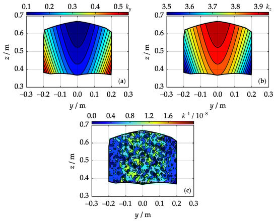
Figure 14. Stiffness maps for the case when the adjacent branches coincide ($y_1=y_2=255\mathrm{mm}$; $\phi =0^{\circ }$): (a) lateral stiffness $k_y$; (b) vertical stiffness $k_z$; (c) overall stiffness $k^{-1}$.

For each combination of parameters $y_1$ and $y_2$, we computed the average values of the stiffness indices and the workspace area using Equations (25) and (27). Figure 15 illustrates the obtained results. The plots in this figure have a triangular shape because we considered the combinations with $y_1\le y_2$. The results match our previous discussions, and we can draw the following conclusions from these plots:

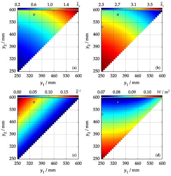
Figure 15. The values of the performance metrics for various parameters $y_1$ and $y_2$ ($\phi =0^{\circ }$): (a) average lateral stiffness ${\overline{k}}_y$; (b) average vertical stiffness ${\overline{k}}_z$; (c) average overall stiffness ${\overline{k}}^{-1}$; (d) workspace area W. The white circles correspond to the initial design with $y_1=255\mathrm{mm}$ and $y_2=505\mathrm{mm}$; the white squares correspond to the optimized design with $y_1=345\mathrm{mm}$ and $y_2=575\mathrm{mm}$.

1.

Average lateral stiffness ${\overline{k}}_y$ increases as sum $y_1+y_2$ increases.

2.

Average vertical stiffness ${\overline{k}}_z$ increases as sum $y_1+y_2$ decreases.

3.

Average overall stiffness ${\overline{k}}^{-1}$ increases as difference $y_2-y_1$ increases.

4.

Workspace area W increases as sum $y_1+y_2$ decreases.

Finally, we performed the multi-objective hierarchical optimization of the design parameters according to Section 3.5. As we discussed earlier, maximizing the lateral stiffness has the highest priority in this optimization problem. However, Figure 15 shows that this objective conflicts with other stiffness indices. In view of the above, we defined the following priority factors for the objective functions:

$$w_1=0.3,w_2=0.5,w_3=0.1,w_4=0.1,$$

(34)

where we set factor $w_2$ for the overall stiffness higher than factor $w_1$ for the lateral stiffness to not sacrifice too much overall stiffness. Scalar factor $\gamma$ was chosen to equal 1.2 after a series of numerical tests.

After the optimization, we obtained the following values of the design parameters: $y_1=345\mathrm{mm}$ and $y_2=575\mathrm{mm}$, corresponding to the white squares in Figure 15. Compared with the initial design parameters $y_1=255\mathrm{mm}$ and $y_2=505\mathrm{mm}$ (the white circles in Figure 15), we have the following results:

1.

Average lateral stiffness ${\overline{k}}_y$ has increased by 54.1%.

2.

Average vertical stiffness ${\overline{k}}_z$ has decreased by 10.3%.

3.

Average overall stiffness ${\overline{k}}^{-1}$ has decreased by 9.9%.

4.

Workspace area W has decreased by 12.1%.

Although the lateral stiffness increased significantly, the values of the other performance metrics became smaller. This decrease, which we consider quite acceptable, is unavoidable because the performance metrics contradict each other. Figure 11a,c, Figure 12a,c, Figure 13a,c illustrate the workspace shapes and stiffness maps for the initial and optimized designs and $\phi =0^{\circ }$. The stiffness maps for other angles $\phi$ have similar behavior, and we omit them for clarity.

This concludes the dimensional synthesis of the considered mechanism. The next section discusses the obtained results and proposed algorithms.

5. Discussion

The symmetric design of the mechanism allowed reducing the number of unknown geometrical parameters to two coordinates of the joints. We achieved this reduction because certain parameters, like the platform width and actuator stroke limits, were predetermined in this study. The values of these parameters also affect the mechanism stiffness. We could include them in the dimensional synthesis problem, but its complexity would grow in this case. On the other hand, the reduced model clearly illustrates how the design parameters impact the performance metrics (Figure 15). A designer can also use the obtained results without solving the multi-objective optimization problem, as we carried out in [27].

The chord method applied to the workspace analysis represents an effective tool for finding the workspace boundary. Unlike conventional discretization approaches [38], it does not need to presample the motion space of the end-effector and check the points outside its workspace. The chord method can also identify other types of workspaces at almost the same level of computational complexity [39]. We used it to compute the reachable and dexterous workspaces of the considered mechanism [26], while [40] applied it to a spatial mechanism. Hay and Snyman [41] showed how to use it for dimensional synthesis without subsequent sampling. The method limitations include computing the voids inside the workspace and treating the so-called bifurcation points, as discussed in [33]. Nonetheless, we believe the chord method is a useful tool for workspace analysis.

Having found the workspace boundary, we reduced the workspace sampling to the point-in-polygon problem. Algorithm 1 is a computationally efficient way to solve this problem because it relies on trivial mathematical operations. In [34], the authors discussed other possibilities for improving this method and presented algorithm variations.

In the next step, we solved the multi-objective optimization problem using the hierarchical $\epsilon$-constraint method. We preferred this method to another commonly used approach, the weighting sum method [42], for several reasons. First, we tried the weighting sum method with various weight values, but it usually gave us the “corner” solutions: $y_1=y_2=595\mathrm{mm}$ (inappropriate because of the zero overall stiffness) or $y_1=255\mathrm{mm}$ and $y_1=595\mathrm{mm}$. In the latter case, lateral stiffness ${\overline{k}}_y$ and overall stiffness ${\overline{k}}^{-1}$ both increase by 51.8% and 33.9%, respectively, while vertical stiffness ${\overline{k}}_z$ and workspace area W decrease by 9.8% and 16.5%. At first glance, these results appear more attractive compared with the hierarchical method. However, with these geometrical parameters, the workspace has almost a triangular shape, less suitable for practical applications. The hierarchical approach is more versatile because it allows us to obtain “intermediate” solutions. Its other benefit over the weighting sum method is that we do not need to normalize objective functions. Article [37] analyzes both methods in more detail.

Summarizing the performed research, we can mention the following directions for future studies that could improve the proposed algorithms and obtained results:

• Enhancing the stiffness model. In Section 3.3, we assumed the drives were the only source of mechanism compliance. We can achieve more accurate results if we consider the stiffness of the revolute joints, moving plate, cylinders, and pistons.
• Modifying the optimization algorithm. In Section 3.5, we solved the multi-objective optimization problem with the hierarchical approach and assigned a priority factor to each objective. Instead of setting these factors, it looks more attractive to a designer to explicitly specify the decrease rate of the low-priority objectives.
• Experimental validation. The theoretical results presented in Section 4 look reasonable, but they have not been verified in practice yet. To validate the results, we plan to estimate the end-effector displacements under the specified load using external measurement systems (e.g., a laser tracker or interferometer).

6. Conclusions

This paper performed the multi-objective dimensional synthesis of a 3-DOF planar parallel mechanism, which constitutes a part of a 5-DOF parallel–serial manipulator and affects its performance. The synthesis problem aimed to find the geometrical parameters of this mechanism that would increase its lateral stiffness. We reduced the number of these parameters to two and introduced various metrics to evaluate stiffness. To compute the mechanism workspace, we proposed a combination of the chord and sampling methods. Finally, we solved the optimal design problem using the hierarchical method.

The results show that the average lateral stiffness of the mechanism increased by 54.1%. Other performance metrics that include the average vertical stiffness, the average overall stiffness, and the workspace area decreased by 10.3%, 9.9%, and 12.1%, respectively. This decrease is caused by the conflicting nature of the performance metrics, and we find it quite acceptable. In future studies, we will develop more accurate stiffness models and perform experimental verification of the obtained results.

References

- Russo, M.; Zhang, D.; Liu, X.J.; Xie, Z. A review of parallel kinematic machine tools: Design, modeling, and applications. Int. J. Mach. Tools Manuf. 2024, 196, 104118. [Google Scholar] [CrossRef]
- Qin, X.; Li, Y.; Feng, G.; Bao, Z.; Li, S.; Liu, H.; Li, H. A novel surface topography prediction method for hybrid robot milling considering the dynamic displacement of end effector. Int. J. Adv. Manuf. Technol. 2024, 130, 3495–3508. [Google Scholar] [CrossRef]
- Lin, C.; Guang, C.; Zheng, Y.; Ma, K.; Yang, Y. Preliminary evaluation of a novel vision-guided hybrid robot system for capsulotomy in cataract surgery. Displays 2022, 74, 102262. [Google Scholar] [CrossRef]
- Tao, B.; Feng, Y.; Fan, X.; Lan, K.; Zhuang, M.; Wang, S.; Wang, F.; Chen, X.; Wu, Y. The accuracy of a novel image-guided hybrid robotic system for dental implant placement: An in vitro study. Int. J. Med. Robot. Comput. Assist. Surg. 2023, 19, e2452. [Google Scholar] [CrossRef] [PubMed]
- Huang, T.; Li, Z.; Li, M.; Chetwynd, D.G.; Gosselin, C.M. Conceptual design and dimensional synthesis of a novel 2-DOF translational parallel robot for pick-and-place operations. J. Mech. Des. 2004, 126, 449–455. [Google Scholar] [CrossRef]
- Zou, Q.; Zhang, D.; Huang, G. Kinematic models and the performance level index of a picking-and-placing hybrid robot. Machines 2023, 11, 979. [Google Scholar] [CrossRef]
- Giri, G.S.; Maddahi, Y.; Zareinia, K. An application-based review of haptics technology. Robotics 2021, 10, 29. [Google Scholar] [CrossRef]
- Tang, Z.; Payandeh, S. Experimental studies of a novel 6-DOF haptic device. In Proceedings of the 2013 IEEE International Conference on Systems, Man, and Cybernetics, Manchester, UK, 13–16 October 2013; pp. 3372–3377. [Google Scholar] [CrossRef]
- Kumar, S.; Wöhrle, H.; de Gea Fernández, J.; Müller, A.; Kirchner, F. A survey on modularity and distributivity in series-parallel hybrid robots. Mechatronics 2020, 68, 102367. [Google Scholar] [CrossRef]
- Feller, D.; Siemers, C. Mechanical design and analysis of a novel three-legged, compact, lightweight, omnidirectional, serial–parallel robot with compliant agile legs. Robotics 2022, 11, 39. [Google Scholar] [CrossRef]
- Li, Q.; Yang, C.; Xu, L.; Ye, W. Performance Analysis and Optimization of Parallel Manipulators; Springer: Singapore, 2023. [Google Scholar] [CrossRef]
- Xu, D.; Dong, J.; Wang, G.; Cai, J.; Wang, H.; Yin, L. Redundant composite polishing robot with triangular parallel mechanism-assisted polishing to improve surface accuracy of thin-wall parts. J. Manuf. Process. 2024, 124, 147–162. [Google Scholar] [CrossRef]
- Gao, J.S.; Li, M.X.; Li, Y.Y.; Wang, B.T. Singularity analysis and dimensional optimization on a novel serial-parallel leg mechanism. Procedia Eng. 2017, 174, 45–52. [Google Scholar] [CrossRef]
- Liu, H.; Huang, T.; Mei, J.; Zhao, X.; Chetwynd, D.G.; Li, M.; Hu, S.J. Kinematic design of a 5-DOF hybrid robot with large workspace/limb–stroke ratio. J. Mech. Des. 2007, 129, 530–537. [Google Scholar] [CrossRef]
- Jin, Y.; Bi, Z.M.; Liu, H.T.; Higgins, C.; Price, M.; Chen, W.H.; Huang, T. Kinematic analysis and dimensional synthesis of Exechon parallel kinematic machine for large volume machining. J. Mech. Robot. 2015, 7, 041004. [Google Scholar] [CrossRef]
- Xu, Y.; Ni, S.; Wang, B.; Wang, Z.; Yao, J.; Zhao, Y. Design and calibration experiment of serial–parallel hybrid rotary platform with three degrees of freedom. Proc. Inst. Mech. Eng. Part C J. Mech. Eng. Sci. 2019, 233, 1807–1817. [Google Scholar] [CrossRef]
- Zhang, D.S.; Xu, Y.D.; Yao, J.T.; Zhao, Y.S. Analysis and optimization of a spatial parallel mechanism for a new 5-DOF hybrid serial-parallel manipulator. Chin. J. Mech. Eng. 2018, 31, 54. [Google Scholar] [CrossRef]
- Xu, L.; Chai, X.; Ding, Y. Design of a 2RRU-RRS parallel kinematic mechanism for an inner-cavity machining hybrid robot. J. Mech. Robot. 2024, 16, 054501. [Google Scholar] [CrossRef]
- Yu, G.; Wu, J.; Wang, L.; Gao, Y. Optimal design of the three-degree-of-freedom parallel manipulator in a spray-painting equipment. Robotica 2020, 38, 1064–1081. [Google Scholar] [CrossRef]
- Dong, C.; Liu, H.; Xiao, J.; Huang, T. Dynamic modeling and design of a 5-DOF hybrid robot for machining. Mech. Mach. Theory 2021, 165, 104438. [Google Scholar] [CrossRef]
- Li, J.; Ye, F.; Shen, N.; Wang, Z.; Geng, L. Dimensional synthesis of a 5-DOF hybrid robot. Mech. Mach. Theory 2020, 150, 103865. [Google Scholar] [CrossRef]
- Xu, P.; Li, B.; Cheung, C.F.; Zhang, J.F. Stiffness modeling and optimization of a 3-DOF parallel robot in a serial-parallel polishing machine. Int. J. Precis. Eng. Manuf. 2017, 18, 497–507. [Google Scholar] [CrossRef]
- Gao, Z.; Zhang, D. Performance analysis, mapping, and multiobjective optimization of a hybrid robotic machine tool. IEEE Trans. Ind. Electron. 2015, 62, 423–433. [Google Scholar] [CrossRef]
- Deng, F.; Liu, X.; Zhang, N.; Zhang, F. Dimension synthesis of a 3T2R labelling robot with hybrid mechanism. J. Eur. Syst. Autom. 2019, 52, 509–514. [Google Scholar] [CrossRef]
- Li, C.; Wu, H.; Eskelinen, H. Design and multi-objective optimization of a dexterous mobile parallel mechanism for fusion reactor vacuum vessel assembly. IEEE Access 2021, 9, 153796–153810. [Google Scholar] [CrossRef]
- Antonov, A.V.; Chernetsov, R.A.; Ulyanov, E.E.; Ivanov, K.A. Use of the chord method for analyzing workspaces of a parallel structure mechanism. IOP Conf. Ser. Mater. Sci. Eng. 2020, 747, 012079. [Google Scholar] [CrossRef]
- Antonov, A. Stiffness evaluation and dimensional synthesis of a 5-DOF parallel-serial robot. In Mechanism Design for Robotics; Lovasz, E.C., Ceccarelli, M., Ciupe, V., Eds.; Springer: Cham, Switzerland, 2024; pp. 99–107. [Google Scholar] [CrossRef]
- Lynch, K.M.; Park, F.C. Modern Robotics: Mechanics, Planning, and Control; Cambridge University Press: Cambridge, UK, 2017. [Google Scholar] [CrossRef]
- Dai, J.S.; Sun, J. Geometrical revelation of correlated characteristics of the ray and axis order of the Plücker coordinates in line geometry. Mech. Mach. Theory 2020, 153, 103983. [Google Scholar] [CrossRef]
- Rosyid, A.; El-Khasawneh, B.; Alazzam, A. Review article: Performance measures of parallel kinematics manipulators. Mech. Sci. 2020, 11, 49–73. [Google Scholar] [CrossRef]
- Wu, J.; Wang, J.; Wang, L.; You, Z. Performance comparison of three planar 3-DOF parallel manipulators with 4-RRR, 3-RRR and 2-RRR structures. Mechatronics 2010, 20, 510–517. [Google Scholar] [CrossRef]
- Gosselin, C. Stiffness mapping for parallel manipulators. IEEE Trans. Robot. Autom. 1990, 6, 377–382. [Google Scholar] [CrossRef]
- Hay, A.M.; Snyman, J.A. The chord method for the determination of nonconvex workspaces of planar parallel manipulators. Comput. Math. Appl. 2002, 43, 1135–1151. [Google Scholar] [CrossRef]
- Hormann, K.; Agathos, A. The point in polygon problem for arbitrary polygons. Comput. Geom. Theory Appl. 2001, 20, 131–144. [Google Scholar] [CrossRef]
- Gunantara, N. A review of multi-objective optimization: Methods and its applications. Cogent Eng. 2018, 5, 1502242. [Google Scholar] [CrossRef]
- Pereira, J.L.J.; Oliver, G.A.; Francisco, M.B.; Cunha Jr, S.S.; Gomes, G.F. A review of multi-objective optimization: Methods and algorithms in mechanical engineering problems. Arch. Comput. Methods Eng. 2022, 29, 2285–2308. [Google Scholar] [CrossRef]
- Grodzevich, O.; Romanko, O. Normalization and other topics in multi-objective optimization. In Proceedings of the Fields-MITACS Industrial Problems Workshop, Toronto, ON, Canada, 14–18 August 2006; pp. 89–101. [Google Scholar]
- Zhou, Y.; Niu, J.; Liu, Z.; Zhang, F. A novel numerical approach for workspace determination of parallel mechanisms. J. Mech. Sci. Technol. 2017, 31, 3005–3015. [Google Scholar] [CrossRef]
- Hay, A.M.; Snyman, J.A. A multi-level optimization methodology for determining the dextrous workspaces of planar parallel manipulators. Struct. Multidiscip. Optim. 2005, 30, 422–427. [Google Scholar] [CrossRef]
- Rashoyan, G.; Shalyukhin, K.; Antonov, A.; Aleshin, A.; Skvortsov, S. Analysis of the structure and workspace of the Isoglide-type robot for rehabilitation tasks. In Advances in Artificial Systems for Medicine and Education III; Hu, Z., Petoukhov, S., He, M., Eds.; Springer: Cham, Switzerland, 2020; pp. 186–194. [Google Scholar] [CrossRef]
- Hay, A.M.; Snyman, J.A. The optimal synthesis of parallel manipulators for desired workspaces. In Advances in Robot Kinematics; Lenarčič, J., Thomas, F., Eds.; Springer: Dordrecht, The Netherlands, 2002; pp. 337–346. [Google Scholar] [CrossRef]
- Marler, R.T.; Arora, J.S. The weighted sum method for multi-objective optimization: New insights. Struct. Multidiscip. Optim. 2010, 41, 853–862. [Google Scholar] [CrossRef]
Disclaimer/Publisher’s Note: The statements, opinions and data contained in all publications are solely those of the individual author(s) and contributor(s) and not of MDPI and/or the editor(s). MDPI and/or the editor(s) disclaim responsibility for any injury to people or property resulting from any ideas, methods, instructions or products referred to in the content. |
© 2024 by the author. Licensee MDPI, Basel, Switzerland. This article is an open access article distributed under the terms and conditions of the Creative Commons Attribution (CC BY) license (https://creativecommons.org/licenses/by/4.0/).