A Simplified Kinematics and Kinetics Formulation for Prismatic Tensegrity Robots: Simulation and Experiments

Abstract

Tensegrity robots offer several advantageous features, such as being hyper-redundant, lightweight, shock-resistant, and incorporating wire-driven structures. Despite these benefits, tensegrity structures are also recognized for their complexity, which presents a challenge when addressing the kinematics and dynamics of tensegrity robots. Therefore, this research paper proposes a new kinematic/kinetic formulation for tensegrity structures that differs from the classical matrix differential equation framework. The main contribution of this research paper is a new formulation, based on vector differential equations, which can be advantageous when it is convenient to use a smaller number of state variables. The limitation of the proposed kinematics and kinetic formulation is that it is only applicable for tensegrity robots with prismatic structures. Moreover, this research paper presents experimentally validated results of the proposed mathematical formulation for a six-bar tensegrity robot. Furthermore, this paper offers an empirical explanation of the calibration features required for successful experiments with tensegrity robots.

1. Introduction and Related Work

A tensegrity structure (see Figure 1) can be defined as a truss-like system that includes elements able to transmit loads in a single direction in space: these are struts/bars (compression members) and wires/cables (tension members). The connections between elements are constituted by ball joints, which also represent the only points at which external loads can be applied. As a consequence, all elements of a tensegrity structure can be loaded only axially, which on the one hand simplifies their modeling, and on the other hand allows one to choose element geometry and materials specialized for axial loads [1], enabling “the creation of structures with high rigidity per unit mass” [2]. Due to its structure, a tensegrity can easily absorb external forces and shocks [3]: for example, NASA proposed a mobile robot based on a ball-shaped tensegrity structure with shock-absorbing features [4]. The first research work on tensegrity systems focused on the study of structure equilibrium and stability analysis [5]. The calculation of the initial equilibrium state of a tensegrity structure, which is in itself a nontrivial task, is termed as “form-finding” [6,7,8]. Recently, researchers have introduced a numerical approach for determining the stability of general structures when their structural stiffness matrix K is positive semi-definite. This stability is defined as the structure’s ability to return to its original state after the application of a small external load [9,10].

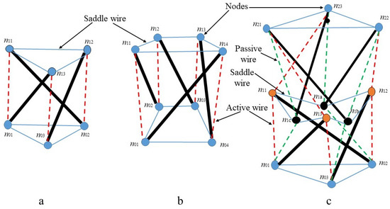
Figure 1. Prismatic tensegrity robot structures: (a) single segment triangular prismatic structure, (b) single segment quadrangular prismatic tensegrity, and (c) dual segment triangular prismatic structure with two layers.

1.1. Tensegrity Kinematics and Kinetics

Tensegrity kinematics is a challenging problem, as it is more complex than serial robot kinematics. Indeed, a tensegrity robot is made of a network of strings and bars with complex wire routing, and inherently has a parallel and closed linkage architecture resulting in complex forward kinematics [11] with structural constraints [12]. One of the most popular methods of solving forward kinematics, consisting of an iterative approach, is the Newton–Raphson method [13]. Alternative methods have been proposed based on genetic algorithms [14,15], potential energy [16,17], and deformation kinematics [18]. Another proposed kinematics formulation for a tensegrity robot structure is the deformation kinematics method. This method imposes nodes in Euclidean space that are described by the nodal coordinates with respect to an inertial Cartesian coordinate system. Position of the joints is defined by deformed or stretched truss elements with respect to the initial position [18]. This is a nontrivial task, as the form of the tensegrity structure should be symmetric in terms of wire tensions. Finding the initial form of the robot after moving is also a crucial task. There are some mechanical factors that deeply affect form-finding, such as friction. The whole mechanism is driven by wires and has some contact between wires and robot rigid components, which yields friction, causing a negative effect on the robot motion, and requires more motor torque than it should [19,20,21,22,23,24].

A problem related to kinematics is that of determining the kinetics of a tensegrity structure. Methods that account for the deformability of bars were described in [18,25,26]. A method based on a mixed Lagrangian–Eulerian approach was presented in [18] to derive the linearized equation of motion around equilibrium configurations for modal analysis and numerical simulation. Another approach to obtain linearized equations of motion was introduced in [25] utilizing second-order ordinary differential equations, which simplified the problem as compared to using partial differential equations, as in [18]. The major drawback of the method in [25] is the large number of parameters required for calculations, related to Young’s modulus and geometrical properties. Finally, the method in [26] directly handles nonlinear tensegrity dynamics.

The most significant and well-known studies on tensegrity are those of Skelton and co-workers. In their formulation, the bars in the tensegrity are considered as rigid bodies, and the nonlinear dynamics of the structure are represented using node, bar, and string connectivity matrices [27]. For example, the node matrix includes the coordinates in the Cartesian space of all nodes (i.e., endpoints of bars) of the structure: it has three rows and a number of columns equal to twice the number of bars. A dynamical model that employs such a formulation has a number of states equal to 12 times the number of bars (i.e., position and velocity coordinates of all bar nodes in the Cartesian space). This is a non-minimal set of coordinates, as the tensegrity dynamics is described using six degrees of freedom for each bar, instead of the minimal number, i.e., five (see, e.g., [18,25,26]). This might seem to be a disadvantage compared to frameworks based on minimal coordinates; however, Skelton’s formalism has some remarkable advantages. First, it avoids using long chains of trigonometric functions, as the only nonlinearities in the dynamic equations are ratios and square roots. Second, the mass matrix of the system, although of larger size, becomes constant, which simplifies certain calculations (mainly, its inversion).

Skelton’s formalism has been used in several studies. For example, a unified formulation of the dynamics of general class-k tensegrity systems—we say that tensegrity is of class-k when it has a maximum of k is rigid bars connected by ball joints—was studied in [28,29]. In [30], the formulation of [29] was extended to account for the presence of damping forces and forces along connected strings passing through several nodes. A related framework was proposed by Goyal et al. [31] to simulate tensegrity dynamics in the presence of rigid bars and massive strings, allowing one to distribute the mass of the strings into a number of point masses along the string, at the same time preserving the exact dynamics of the rigid bars. Finally, a software toolbox for static analysis and simulation of the dynamics of tensegrity systems based on the modeling framework of [31] was created and is described in [32].

The kinematics of tensegrity structures pose a challenge due to the need for simultaneous motor control, whereas serial manipulators with rigid links only require control of individual motors [33]. The wire-net structure of tensegrity robots makes them susceptible to movements and shocks from any of its actuators, whereas kinematics in serial manipulators are based on their degrees of freedom [34,35]. Tensegrity structures have a large number of structural constraints, making kinematic formulation based on constraint equations necessary to achieve the desired degrees of freedom, unlike the simpler kinematics formulation in serial manipulators.

1.2. Prismatic Tensegrity Structures

A recent survey paper [36] classified tensegrity robots into different classes: prismatic [37], spherical [38,39], humanoid musculoskeletal [40,41,42], and bio-inspired [43]. Prismatic tensegrity robots (see Figure 1) that are based on the composition of so-called tensegrity prisms constitute one of the most popular solutions adopted to date, which facilitates stability, symmetry, and self-equilibrium. A tensegrity prism is composed of p struts and, usually, at least $3p$ strings that form p-sided polygons on the top and bottom, such as triangular tensegrity prism with 3 struts and 9 strings, and quadrilateral tensegrity prism with 4 struts and 12 strings’ [36]. Triangular and quadrilateral prisms (i.e., $p=3$ and $p=4$, respectively) constitute the simplest and most commonly used designs. The fact that prismatic tensegrity structures usually consist of repeating patterns makes it possible to also use a simplified assembly sequence. Prismatic tensegrity structures have been utilized to create tensegrity robots equivalent to industrial robot arms with open-chain kinematic structure [44,45]. Due to their lightweight components (i.e., bars and strings) and parallel architecture, these robots can manipulate higher payloads, relative to their weight, as compared to traditional industrial manipulators [36]. Tensegrity robots are well-suited for operating in uneven and unstructured environments, as they do not require additional infrastructure and facilities, thus reducing the cost of exploitation [46]. Despite these advantages, tensegrity robots cannot achieve high-speed operation comparable to delta manipulators with a parallel structure [47,48]. On the other hand, compared to wire-driven robots such as continuum manipulators [49,50], tensegrity robots have a significantly higher payload capacity.

1.3. Contribution and Paper Structure

This paper presents a new kinematics and kinetics formulation for prismatic tensegrity robots with rigid bars, massless strings, and base nodes fixed to the ground, which uses a minimal set of coordinates. Our kinematics formulation (which presents similarities with the Denavit–Hartenberg convention for robot kinematics) employs Euler angles and homogeneous transformations to express spatial rotation and translation of the node coordinates. Then, the proposed kinetics formulation defines the equations of motion via gravitational torque vectors. In a prismatic tensegrity structure with base nodes fixed to the ground, it is easy to define the direction of the gravitational force vector, unlike, e.g., in ball-shape tensegrity structures where the direction of the gravitational force vector may change with time. The considered kinetics formulation requires basic parameters, such as wire tensions, bar lengths, bar masses, end plate mass, and gravitation constant. The kinematics and kinetics formulation proposed in this work can also be seen as a preliminary step towards the determination of a dynamical model of prismatic tensegrity robots with a minimal set of coordinates. The obvious advantage of such a model over non-minimal coordinate systems would be the presence of a smaller number of variables. The drawbacks would be its limitation to prismatic structures (only the formulation for triangular prisms is explicitly considered), the presence of long chains of products of trigonometric functions, and the need to calculate a symbolic expression of the inverse of the mass matrix, in order to simulate the system dynamics. In certain contexts, this formulation can be advantageous with respect to non-minimal coordinate systems: for example, if the motion of a tensegrity robot has to be planned by numerical optimal control (using optimization solvers based on sequential quadratic programming [51] or interior point methods [52]), then the presence of an arbitrary number of sines and cosines (which are infinitely differentiable with respect to their argument) would be preferable to the presence of square roots (which are found in non-minimal coordinates formulations and are in general non-differentiable). In addition, for the same type of solvers, the presence of a smaller number of decision variables in the optimal control problem would be preferable in case the solver is not designed to exploit the sparsity pattern deriving from the non-minimal coordinate system: indeed, several software toolboxes exist that can account for sparsity in optimal control problems (e.g., [53,54]), but none of them is designed for the specific sparsity patterns of non-minimal tensegrity coordinate systems. The proposed kinematic and kinetic formulation, as noted above, is applicable to prismatic tensegrity structures with fixed and movable top plates, such as triangular and quadrangular prismatic tensegrity structures.

The paper is organized as follows. Section 2 introduces the specific tensegrity robot that will be used as a case study to illustrate the details of our modeling framework. Section 3 will be devoted to the derivation of kinematics and dynamics, whereas the experimental validation will be presented in Section 4. Conclusions will be drawn in Section 5.

2. Case Study

To introduce and then experimentally validate our kinematics and kinetics formulation, we designed a triangular prismatic tensegrity robot with pulley-guided wire-driven actuation (see Figure 2). The robot structure (see Figure 3) consists of two plates at the bottom and the top (represented as grey surfaces), six bars (thick green, blue, and orange lines), and a number of wires, represented as thinner lines, either solid or dashed. A total of 12 nodes are present, divided into three sets: base nodes ($n_{01},n_{02}$ and $n_{03}$), mid nodes ($n_{11},n_{12},n_{13}$ and $n_{1a},n_{1b},n_{1c}$), and end nodes ($n_{21},n_{22},n_{23}$). The joints at the base nodes are universal joints (with two degrees of freedom); at the locations of the mid nodes, wires are connected to bars via a wire-guiding pulley (3D-printed except for the ball bearings inside them); finally, the joint at the end nodes consist of spherical joints with 2 degrees of freedom because upper nodes are directly connected to the active and passive wires, which constraints rotational motion along the z-axis. Therefore upper node joints in the mathematical formulation will be considered as universal joints. The robot is actuated by three driving wires controlled by individual electric motors (see Figure 2). To provide rigidity and static stability, three passive wires were inserted in the structure (shown as dashed green lines in Figure 3), whose pretension is adjustable via individual extension springs. A saddle wire (solid blue line in Figure 3) is also utilized to ensure the static balance of the structure.

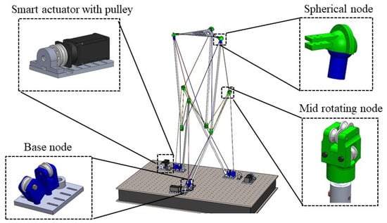
Figure 2. The computer-aided design model of the prismatic tensegrity robot with triangular base.

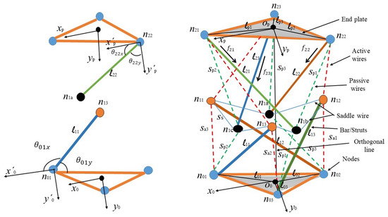
Figure 3. Annotated schematics of the prismatic tensegrity robot. Thick blue, orange, and green solid lines are solid bars. Dotted orange lines are driving wires; dotted green lines are passive wires. The solid blue line is the saddle wire. Base and end-plate nodes are blue-filled circles. Black and orange-filled circles are middle nodes (universal joints).

Experimental Setup and Initial Posture Calibration

In addition to the fixed parameters such as the lengths of the bars, the robot form primarily depends on wire tension. In our prototype (shown in Figure 4), we use three types of wires: active, passive, and saddle (also passive) wires. The three active wires are directly connected to the electric motors, the three passive wires are connected to the extension springs on the base for providing rigidity to the robot structure, and the saddle wire sustains the weight of the upper layer and allows the kinetic balance of the whole structure. In Figure 4, one can notice the presence of cameras: these are part of an Optitrack motion capture system, which allows us to obtain high-precision data for node positions, mainly used to experimentally validate our models.

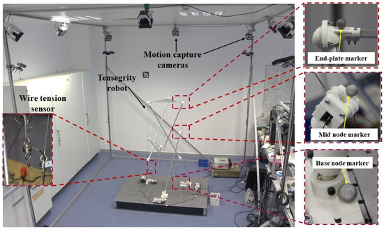
Figure 4. Tensegrity robot experimental setup with zoomed components inside the motion capture area.

When running experiments involving robot motion, specific angular position references were given to the motors (Dynamixel PRO H54-200-S500-R, Seoul, Korea) that actuated the active wires. The control environment consisted of two independent parts. The first was the robot control structure, implemented on a PC with Intel Core i9 CPU and 16 GB RAM via Robot Operating System (ROS) Kinetic running under Ubuntu 16.04 LTS; the ROS environment integrated tension sensors readings, electric motors, and control code. The second was implemented on a different PC with an Intel Core i3 CPU and 8 GB RAM running Windows 8 and used to measure the robot trajectory with the Optitrack motion capture system via the Motive software. In order to obtain readings from the Optitrack system, reflective markers were embedded on tensegrity robot nodes, as shown in Figure 4. A total of 12 infrared diffusing markers were used, one for each node of the structure.

To measure wire tension, we installed seven tension sensors (Flintec Y1, Hudson, USA), one for each wire, also shown in Figure 4. The analog output of each tension sensor is fed into an amplifier module, and the corresponding amplified signal is acquired by the analog input of a microcontroller (Arduino Uno, Italy). This microcontroller sends the measurements via a universal serial bus (USB) to the ROS workstation.

Posture calibration is achieved by using data from the tension sensors by satisfying two main requirements:

• The line that connects the centers of the upper plate and base plate should be perpendicular to the ground while the upper plate is kept on a horizontal plane.
• Each node in the upper plate is connected to one active wire and one passive wire. Defining the corresponding initial tensions $s_{a1}^{init}$, $s_{a2}^{init}$, $s_{a3}^{init}$ for active wires and $s_{p1}^{init}$, $s_{p2}^{init}$, $s_{p3}^{init}$ for passive wires, the following condition should be satisfied:

  $$s_{a1}^{init}+s_{p1}^{init}=s_{a2}^{init}+s_{p2}^{init}=s_{a3}^{init}+s_{p3}^{init}.$$

  (1)

3. Proposed Formulation of Tensegrity Kinematics and Kinetics

In this section we formulate the kinematics and kinetics of a class of prismatic tensegrity robots that include the one in our case study. In more detail, we consider triangular prismatic tensegrity structures with six bars and two triangular plates.

3.1. Node Coordinates

As a preliminary step, we introduce the rotation matrices for an angle $\theta$ around the x, y, and z axes of a generic right-handed reference frame as

$$e^{\widehat{i}\theta }=\left(\begin{array}{ccc}1& 0& 0\\ 0& cos\theta & -sin\theta \\ 0& sin\theta & cos\theta \end{array}\right),e^{\widehat{j}\theta }=\left(\begin{array}{ccc}cos\theta & 0& sin\theta \\ 0& 1& 0\\ -sin\theta & 0& cos\theta \end{array}\right),e^{\widehat{k}\theta }=\left(\begin{array}{ccc}cos\theta & sin\theta & 0\\ -sin\theta & cos\theta & 0\\ 0& 0& 1\end{array}\right),$$

(2)

where $\widehat{i}$, $\widehat{j}$, and $\widehat{k}$ are skew-symmetric matrices of the unit vectors $i,j,$ and k of the axes x, y, and z, respectively. Specifically, we will use two reference frames, both shown in Figure 3: the first, namely $O_0-x_0{y}_0{z}_0$, is a fixed frame with origin at the center of the base plate; the second, $O_p-x_p{y}_p{z}_p$, is a moving frame attached to the top plate, with its origin at the center of this plate.

We will now detail how to obtain each of the column vectors that define the coordinates of each node of the prismatic tensegrity robot in the $O_0-x_0{y}_0{z}_0$ frame. We can express the coordinates of the nodes in the base plate as

$$n_{0i}=e^{\widehat{k}(i-1)(-\frac{2\pi }{3})}\begin{array}{ccc}({\ell }_{0i}& 0& {0)}^T\end{array}=e^{-\widehat{k}{\theta }_{0i}}\begin{array}{ccc}({\ell }_{0i}& 0& {0)}^T,i=1,2,3,\end{array}$$

(3)

where ${\ell }_{0i}$, as indicated in Figure 3, is the distance between the plate center and $n_{0i}$. The angle ${\theta }_{0i}$ is to account for irregular triangles, and in our case of an equilateral base triangle, we can write ${\theta }_{0i}=(i-1)\left(\frac{2\pi }{3}\right)$.

To define the positions of the mid nodes, we first introduce ${\theta }_{0ix}$ and ${\theta }_{0iy}$ as the two rotation angles that describe the orientation of the universal joint at the nodes $n_{0i},(i=1,2,3)$, starting from an upper vertical orientation in the $O_0-x_0{y}_0{z}_0$ frame. Using these angles, we can determine the position of the three mid nodes corresponding to the upper node on each of the three corresponding bars:

$$n_{1i}=n_{0<i>}+e^{\widehat{i}{\theta }_{0<i>x}}{e}^{\widehat{j}{\theta }_{0<j>y}}\begin{array}{ccc}(0& 0& {\ell }_{1<i>}{)}^T,i=1,2,3,\end{array}$$

(4)

where $<1>\triangleq 2$, $<2>\triangleq 3$, and $<3>\triangleq 1$.

Three nodes of the top triangle plate are assumed to take positions such that

$$n_{2i}=n_{up}+e^{{\widehat{i}\varphi }_{px}}{e}^{{\widehat{j}\varphi }_{py}}{e}^{\widehat{k}\varphi (pz+rpi)}\begin{array}{ccc}(l_{pi}& 0& {0)}^T,\end{array}$$

(5)

$(i=1,2,3)$ and $(rp1=-\frac{\pi }{3},rp2=\pi ,rp3=\frac{\pi }{3})$, where $u_p={\left(u_{px}{u}_{py}{u}_{pz}\right)}^T$ is the position of the upper plate origin $Op$, and ${\varphi }_{px},{\varphi }_{py},{\varphi }_{pz}$ are tilting angle of the top-plate with respect to the base frame.

Then, the node positions at the other extremities of the bars connected to the top plate can be written as:

$$n_{1p}=n_{2<\rho >}-e^{{\widehat{i}\varphi }_{px}}{e}^{{\widehat{j}\varphi }_{py}}{e}^{{\widehat{k}\varphi }_{pz}}{e}^{\widehat{i}{\theta }_{2<\rho >x}}{e}^{\widehat{j}{\theta }_{2<\rho >y}}{\left(\begin{array}{ccc}0& 0& {\ell }_{2<\rho >}\end{array}\right)}^T,\rho =a,b,c,$$

(6)

where $<a>=2,<b>=1,<c>=3$, and ${\theta }_{2<\rho >x}$ and ${\theta }_{2<\rho >y}$, with $\rho =a,b,c$, are the two rotation angles that describe the orientation of the universal joint at nodes $n_{2<\rho >}$, starting from a lower vertical orientation in the $O_p-x_p{y}_p{z}_p$ frame.

3.2. Definition of the Constraint Equations

To describe the configuration of the prismatic tensegrity robot, the following 22 variables have to be determined via kinematics and kinetics:

(a)

Three coordinates describing the position of the center of the top plate:

$$u_p={\left(\begin{array}{ccc}{u}_{px}& u_{py}& u_{pz}\end{array}\right)}^T;$$

(b)

Three angles describing the rotation of the top plate:

$${\varphi }_p={\left(\begin{array}{ccc}{\varphi }_{px}& {\varphi }_{py}& {\varphi }_{pz}\end{array}\right)}^T;$$

(c)

Twelve angles defining the rotation of the six universal joints:

$${\theta }_{01x},{\theta }_{01y},{\theta }_{02x},{\theta }_{02y},{\theta }_{03x},{\theta }_{03y},{\theta }_{21x},{\theta }_{21y},{\theta }_{22x},{\theta }_{22y},{\theta }_{23x},{\theta }_{23y};$$

(d)

Three forces $f_{21},f_{22},f_{23}$, defining the axial forces of the bars connected to the top plate;

(e)

The (scalar) tension of the saddle wire $s_s$.

To determine these variables, we formulate 22 constraint equations (CEs) that describe the kinematic and kinetic equilibrium state in the presence of external forces (i.e., gravity and forces applied by the motors at the robot base to the active wires). In this research, the tensegrity robot driving parameter is an active wire tension, and feedback values of wire tension are obtained via tension sensors. In these equations, $s_{a1}$, $s_{a2}$, and $s_{a3}$ indicate the tension of each active wire, whereas $s_{p1}$, $s_{p2}$, and $s_{p3}$ indicate the tension of each passive wire. In order to simplify calculations, the latter will be considered as constant. This approximation is realistic whenever the range of motion of the system is not of a very significant entity. We divide the CEs into six groups:

• (CE1) The magnitude of moment vectors at the nodes $n_{01}$, $n_{02}$, and $n_{03}$ applied by bars $l_{11}$, $l_{12}$, and $l_{13}$, respectively, must be zero (three equations).
• (CE2) The magnitude of the moment vectors at nodes $n_{21}$, $n_{22}$, and $n_{23}$ applied by bars $l_{21}$, $l_{22}$, and $l_{23}$, respectively, must be zero (three equations).
• (CE3) The sum of the forces applied to nodes $n_{21},n_{22}$, and $n_{23}$ must be equal to the opposite gravity vector applied to the mass center of the top plate (three equations).
• (CE4) The sum of the force vectors applied to nodes $n_{1a}$, $n_{1b}$, and $n_{1c}$ must be equal to the opposite gravity vector applied to the nodes due to the weight of the end plate and the bars (nine equations).
• (CE5) The resultant moment vector applied to the center of the top plate must be a zero vector (three equations).
• (CE6) The length of the saddle wire is constant (one equation).

In this research, we do not consider the inertia effect because the simulation considers absolutely static balance of force and torque and holonomic kinematic constraints. It does not include dynamic force and torque, which means that no accelerations or angular accelerations are included in the formulations. In the following, we will provide a mathematical formulation of the CEs. All other mathematical symbol notations are shown in Table A1.

3.2.1. Formulation of CE1

The first three equations express that the resultant moments of the external forces at nodes $n_{01}$, $n_{02}$, and $n_{03}$ applied at the other ends of the corresponding bars (i.e., $n_{13}$, $n_{11}$, $n_{12}$) by the active wires must be zero. By referring to these moments as $T_{01}$, $T_{02}$, and $T_{03}$ (see Figure 5), we can write the following expressions:

$$\begin{array}{cc}\hfill T_{01}& =(n_{13}-n_{01})\times \left(s_{a2}((\widehat{n_{21}-n_{13}})+(\widehat{n_{03}-n_{13}}))+s_s((\widehat{n_{1c}-n_{13}})+(\widehat{n_{1b}-n_{13}}))+\frac{m_{L}g}{2}+m_{n}g\right)\hfill \end{array}$$

(7)

$$\begin{array}{cc}\hfill T_{02}& =(n_{11}-n_{02})\times \left(s_{a3}((\widehat{n_{23}-n_{11}})+(\widehat{n_{01}-n_{11}}))+s_s((\widehat{n_{1c}-n_{11}}+(\widehat{n_{1a}-n_{11}}))+\frac{m_{L}g}{2}+m_{n}g\right)\hfill \end{array}$$

(8)

$$\begin{array}{cc}\hfill T_{03}& =(n_{12}-n_{03})\times \left(s_{a1}((\widehat{n_{22}-n_{12}})+(\widehat{n_{02}-n_{12}}))+s_s((\widehat{n_{1b}-n_{12}})+(\widehat{n_{1a}-n_{12}}))+\frac{m_{L}g}{2}+m_{n}g\right)\hfill \end{array}$$

(9)

where $\widehat{n_{22}-n_{12}}\triangleq (n_{22}-n_{12})/|n_{22}-n_{12}|$ (and similarly for all other vectors), $m_L$ is the mass of the bar (equal for all bars), and $g\triangleq {\left(\begin{array}{ccc}0& 0& -9.80665\end{array}\right)}^T$ m/s${}^2$ is the gravity acceleration vector. The CEs derived from (7)–(9) are

$$\begin{array}{ccc}(c_1& c_2& c_3{)}^T\end{array}\equiv \begin{array}{ccc}\left(\right|T_{01}|& |T_{02}|& |T_{03}|{)}^T=0_3^T,\end{array}$$

(10)

where, for any integer k, $0_k\triangleq {\left(\begin{array}{ccc}0& \dots & 0\end{array}\right)}^T\in {\mathbb{R}}^k$.

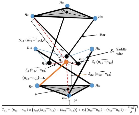
Figure 5. Illustration that shows the terms used for the computation of the torque vector $T_{01}$.

3.2.2. Formulation of CE2

The torque vectors applied at nodes $n_{21},n_{22},n_{23}$ can be written as

$$\begin{array}{c}\hfill T_{21}=(n_{1b}-n_{21})\times \left(s_{p1}((\widehat{n_{22}-n_{1b}})+(\widehat{n_{03}-n_{1b}}))+s_s((\widehat{n_{13}-n_{1b}})+(\widehat{n_{12}-n_{1b}}))+\frac{m_{L}g}{2}+m_{n}g\right)\end{array}$$

(11)

$$\begin{array}{c}\hfill T_{22}=(n_{1a}-n_{22})\times \left(s_{p3}((\widehat{n_{23}-n_{1a}})+(\widehat{n_{02}-n_{1a}}))+s_s((\widehat{n_{11}-n_{1a}})+(\widehat{n_{12}-n_{1a}}))+\frac{m_{L}g}{2}+m_{n}g\right)\end{array}$$

(12)

$$\begin{array}{c}\hfill T_{23}=(n_{1c}-n_{23})\times \left(s_{p2}((\widehat{n_{21}-n_{1c}})+(\widehat{n_{01}-n_{1c}}))+s_s((\widehat{n_{13}-n_{1c}})+(\widehat{n_{11}-n_{1c}}))+\frac{m_{L}g}{2}+m_{n}g\right)\end{array}$$

(13)

The CEs derived from (11)–(13) are

$${\left(\begin{array}{ccc}{c}_4& c_5& c_6\end{array}\right)}^T\equiv {\left(\begin{array}{ccc}|T_{21}|& |T_{22}|& |T_{23}|\end{array}\right)}^T=0_3^T$$

(14)

3.2.3. Formulation of CE3

The difference between the total sum of the forces applied to nodes $n_{21},n_{22}$, and $n_{23}$ and the gravity vector applied to the mass center of the top plate must be equal to zero:

$$\begin{array}{c}{\left(\begin{array}{ccc}{c}_7& c_8& c_9\end{array}\right)}^T\equiv f_{21}(\widehat{n_{21}-n_{1b}})+f_{23}(\widehat{n_{23}-n_{1c}})+f_{22}(\widehat{n_{22}-n_{1a}})\hfill \\ \hspace{1em}\hspace{1em}\hspace{1em}\hspace{1em}\hspace{1em}\hspace{1em}\hspace{0.17em}-s_{p3}(\widehat{n_{23}-n_{1a}})-s_{p1}(\widehat{n_{22}-n_{1b}})-s_{p2}(\widehat{n_{21}-n_{1c}})\hfill \\ \hspace{1em}\hspace{1em}\hspace{1em}\hspace{1em}-s_{a1}(\widehat{n_{22}-n_{12}})-s_{a3}(\widehat{n_{23}-n_{11}})-s_{a2}(\widehat{n_{21}-n_{13}})+m_{tp}g+3m_{n}g=0_3\hfill \end{array}$$

(15)

where $m_{tp}$ is the mass of the top plate. To run the convergence of Newton–Raphson, the force terms in (15) can be defined as

$$\begin{array}{c}\hfill f_{21}=s_{a1}+k_p{l}_{p1i}+\left(\frac{m_{tp}}{3}+m_L+m_n\right)g\\ \hfill f_{22}=s_{a2}+k_p{l}_{p2i}+\left(\frac{m_{tp}}{3}+m_L+m_n\right)g\\ \hfill f_{23}=s_{a3}+k_p{l}_{p3i}+\left(\frac{m_{tp}}{3}+m_L+m_n\right)g\end{array}$$

(16)

where $m_n$ is the node mass, $k_p$ is the spring constant of the passive wires, and $l_{pn}$, $n=1,2,3$, are the lengths of each passive wire, defined as follows:

$$\begin{array}{c}\hfill l_{p1}=|n_{22}-n_{1b}|\hspace{0.17em}+\hspace{0.17em}|n_{03}-n_{1b}|\\ \hfill l_{p2}=|n_{21}-n_{1c}|\hspace{0.17em}+\hspace{0.17em}|n_{01}-n_{1c}|\\ \hfill l_{p3}=|n_{23}-n_{1a}|\hspace{0.17em}+\hspace{0.17em}|n_{02}-n_{1a}|\end{array}$$

(17)

After Equation (17) we can calculate passive wire tension:

$$\begin{array}{c}\hfill s_{p1}=\left(\right|n_{22}-n_{1b}|\hspace{0.17em}+\hspace{0.17em}|n_{03}-n_{1b}|\hspace{0.17em}-\hspace{0.17em}{l}_{p1}+l_{p1i})k_p\\ \hfill s_{p2}=\left(\right|n_{21}-n_{1c}|\hspace{0.17em}+\hspace{0.17em}|n_{01}-n_{1c}|\hspace{0.17em}-\hspace{0.17em}{l}_{p2}+l_{p2i})k_p\\ \hfill s_{p3}=\left(\right|n_{23}-n_{1a}|\hspace{0.17em}+\hspace{0.17em}|n_{02}-n_{1a}|\hspace{0.17em}-\hspace{0.17em}{l}_{p3}+l_{p3i})k_p\end{array}$$

(18)

here, $k_p$ is the spring constant of the passive wire, $l_{p1i},l_{p2i}$, and $l_{p3i}$ are an initial stretch of the passive wire spring.

3.2.4. Formulation of CE4

The difference between the sum of the force vectors applied to nodes $n_{1a}$, $n_{1b}$, and $n_{1c}$ and the gravity vector applied to the nodes due to the weight of the top plate and the bars must be equal to zero:

$$\begin{array}{c}{\left(\begin{array}{ccc}{c}_{10}& c_{11}& c_{12}\end{array}\right)}^T\equiv f_{22}(\widehat{n_{1a}-n_{22}})+s_{p3}((\widehat{n_{23}-n_{1a}})+(\widehat{n_{02}-n_{1a}}))\hfill \\ \hspace{1em}\hspace{1em}\hspace{1em}\hspace{1em}\hspace{1em}\hspace{1em}\hspace{1em}\hspace{1em}\hspace{1em}\hspace{1em}\hspace{1em}+s_s((\widehat{n_{11}-n_{1a}})+(\widehat{n_{12}-n_{1a}}))-(m_n+m_L)g=0_3\hfill \end{array}$$

(19)

$$\begin{array}{c}{\left(\begin{array}{ccc}{c}_{13}& c_{14}& c_{15}\end{array}\right)}^T\equiv f_{21}(\widehat{n_{1b}-n_{21}})+s_{p1}((\widehat{n_{22}-n_{1b}})+(\widehat{n_{03}-n_{1b}}))\hfill \\ \hspace{1em}\hspace{1em}\hspace{1em}\hspace{1em}\hspace{1em}\hspace{1em}\hspace{1em}\hspace{1em}\hspace{1em}\hspace{1em}\hspace{1em}+s_s((\widehat{n_{13}-n_{1b}})+(\widehat{n_{12}-n_{1b}}))-(m_n+m_L)g=0_3\hfill \end{array}$$

(20)

$$\begin{array}{c}{\left(\begin{array}{ccc}{c}_{16}& c_{17}& c_{18}\end{array}\right)}^T\equiv f_{23}(\widehat{n_{1c}-n_{23}})+s_{p2}((\widehat{n_{21}-n_{1c}})+(\widehat{n_{01}-n_{1c}}))\hfill \\ \hspace{1em}\hspace{1em}\hspace{1em}\hspace{1em}\hspace{1em}\hspace{1em}\hspace{1em}\hspace{1em}\hspace{1em}\hspace{1em}\hspace{1em}+s_s((\widehat{n_{11}-n_{1c}})+(\widehat{n_{13}-n_{1c}}))-(m_n+m_L)g=0_3.\hfill \end{array}$$

(21)

3.2.5. Formulation of CE5

The moment vector applied to the center of the top plate must be equal to zero:

$$\begin{array}{c}{\left(\begin{array}{ccc}{c}_{19}& c_{20}& c_{21}\end{array}\right)}^T\hfill \\ \hspace{1em}\hspace{1em}\hspace{1em}\hspace{1em}\equiv (n_{21}-u_p)\times (f_{21}(\widehat{n_{21}-n_{1b}})-s_{a2}(\widehat{n_{21}-n_{13}})-s_{p2}(\widehat{n_{21}-n_{1c}}))\hfill \\ \hspace{1em}\hspace{1em}\hspace{1em}\hspace{1em}+(n_{22}-u_p)\times (f_{22}((\widehat{n_{22}-n_{1a}})-s_{a1}(\widehat{n_{22}-n_{12}})-s_{p1}(\widehat{n_{22}-n_{1b}}))\hfill \\ \hspace{1em}\hspace{1em}\hspace{1em}\hspace{1em}+(n_{23}-u_p)\times (f_{23}((\widehat{n_{23}-n_{1c}})-s_{a3}(\widehat{n_{23}-n_{11}})-s_{p3}(\widehat{n_{23}-n_{1a}}))=0_3\hfill \end{array}$$

(22)

3.2.6. Formulation of CE6

The length of the saddle wire $l_s$ must be equal to the sum of all of its sub-parts, and the related constraint can be written as follows:

$$\begin{array}{c}{c}_{22}\equiv \hspace{0.17em}|n_{11}-n_{1c}|\hspace{0.17em}+\hspace{0.17em}|n_{1c}-n_{13}|\hspace{0.17em}+\hspace{0.17em}|n_{13}-n_{1b}|\hfill \\ \hspace{1em}\hspace{1em}\hspace{1em}\hspace{1em}\hspace{1em}\hspace{1em}\hspace{1em}\hspace{1em}\hspace{1em}\hspace{1em}\hspace{1em}\hspace{1em}\hspace{1em}+\hspace{0.17em}|n_{1b}-n_{12}|\hspace{0.17em}+\hspace{0.17em}|n_{12}-n_{1a}|\hspace{0.17em}+\hspace{0.17em}|n_{1a}-n_{11}|\hspace{0.17em}-\hspace{0.17em}{l}_s=0.\hfill \end{array}$$

(23)

3.3. Inverse Kinematics

The considered tensegrity robot can be described by 22 internal variables, namely ${\theta }_{01x}$, ${\theta }_{01y}$, ${\theta }_{02x}$, ${\theta }_{02y}$, ${\theta }_{03x}$, ${\theta }_{03y}$, ${\theta }_{21x}$, ${\theta }_{21y}$, ${\theta }_{22x}$, ${\theta }_{22y}$, ${\theta }_{23x}$, ${\theta }_{23y}$, $u_{px}$, $u_{py}$, $u_{pz}$, ${\varphi }_{px}$, ${\varphi }_{py}$, ${\varphi }_{pz}$, $f_{21}$, $f_{22}$, $f_{23}$, and $s_s$, which constitute, in the noted order, the components of the system configuration vector $q\in {\mathbb{R}}^{22}$. On the other hand, Equations (7)–(23) form a vector of CEs

$$c_v={(c_1,c_2,\dots ,c_{22})}^T.$$

(24)

Total differentiation of $c_v$ with respect to q and the active wire tension vector $s_a={\left(\begin{array}{ccc}{s}_{a1}& s_{a2}& s_{a3}\end{array}\right)}^T$ gives us

$$\frac{\partial c_v}{\partial q}\Delta q+\frac{\partial c_v}{\partial s_a}\Delta s_a=0_{22}$$

(25)

Since $\frac{\partial c_v}{\partial q}$ is a 22 × 22 square matrix, an infinitesimal update of q yielded by a given variation of active wire tension $\delta s_a$ is calculated by, from (25), the variation of q corresponding to a given variation of active wire tension $\Delta s_a$ can be obtained as:

$$\Delta q=-{(\frac{\partial c}{\partial q})}^{-1}\frac{\partial c}{\partial s_a}\Delta s_a$$

(26)

Let us denote $q_{nt}\in R^{19}$ that excludes the position of the top-plate ${(u_p=u_{px}{u}_{py}{u}_{pz})}^T$ from q.

Total differentiation of $c_v$ with respect to $q_{nt},u_p$, and $s_a$ gives us

$$\frac{\partial c_v}{\partial q_{nt}}\Delta q_{nt}+\frac{\partial c_v}{\partial u_p}\Delta u_p+\frac{\partial c_v}{\partial s_a}\Delta s_a=0_{22}$$

(27)

which can be reformed as

$$(\frac{\partial c_v}{\partial q_{nt}}\frac{\partial c_v}{\partial s_a})\left(\begin{array}{c}\Delta q_{nt}\\ \Delta s_a\end{array}\right)+\frac{\partial c_v}{\partial u_p}\Delta u_p=0_{22}.$$

(28)

Since $(\frac{\partial c_v}{\partial q_{nt}}\frac{\partial c_v}{\partial s_a})$ is a $22\times 22$ square matrix, it can be solved as

$$\left(\begin{array}{c}\Delta q_{nt}\\ \Delta s_a\end{array}\right)=-{(\frac{\partial c_v}{\partial q_{nt}}\frac{\partial c_v}{\partial s_a})}^{-1}\frac{\partial c}{\partial u_p}\Delta u_p.$$

(29)

Equation (27) gives us the tension of the active wires that provides a required infinitesimal moving of the top plate. According to the formulation, the main driving variable is the tension value of the active wire. The wire tension value in Equation (29) derives from $s_a$.

4. Experimental Validation

This section describes the validation of the proposed kinematics and kinetics modeling framework by comparing simulations based on the formulation in Section 3 with the results of experiments. The parameters of our tensegrity robot are reported in Table 1.

Table 1. The initial parameters of the tensegrity robot in the experiments.

Parameters	Symbol	Value
	$l_{11}=l_{12}=l_{13}$
Bar length	$l_{21}=l_{22}=l_{23}$	1000 mm
Triangle length	$l_{01}=l_{02}=l_{03}$	450 mm
Spring constant	$k_p$	1800 N/m
Top plate mass	$m_{tp}$	0.86 kg
Bar mass	$m_L$	0.18 kg
Node mass	$m_n$	0.1 kg
Gravitation vector	g	${\left(\begin{array}{ccc}0& 0& -9.80665\end{array}\right)}^T$ m/s${}^2$
Passive wire tension	$s_{p1}=s_{p2}=s_{p3}$	90 N
Active wire tension	$s_{a1}=s_{a2}=s_{a3}$	65 N
Saddle wire tension	$s_s$	120 N

4.1. Determination of the Initial Posture

First, the initial position of the tensegrity robot structure was replicated in our simulation environment to check the validity of the proposed forward kinematic node positions.

Figure 6 shows the obtained initial posture of the tensegrity robot starting from the values indicated in Table 1. The same values of $s_a$ and $s_p$ were also enforced in the actual experimental setup, thus obtaining a corresponding robot posture. The two postures were compared by reporting the node positions of the simulation and the node positions obtained via motion capture in the experimental setup. The results can be seen in Table 2.

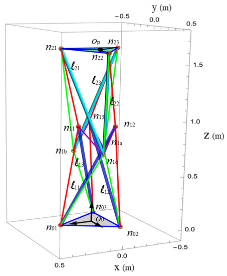
Figure 6. Initial posture of the tensegrity robot.

Table 2. Initial node position for the simulation and experiment.

	Nodes	Simulation			Experiment			Difference
		X (mm)	Y (mm)	Z (mm)	X (mm)	Y (mm)	Z (mm)	X (mm)	Y (mm)	Z (mm)
Base plate	$n_{01}$	250	0	0	267	1	1.6	17	1	1.6
	$n_{02}$	−130	−225	0	−127	−232	1.6	3	7	1.6
	$n_{03}$	−130	225	0	−127	232	1.6	3	7	1.6
Mid nodes	$n_{11}$	144	50	920	148	49	921	4	1	1
	$n_{12}$	−50	−150	920	−56	−148	872	6	2	48
	$n_{13}$	−130	110	910	−120	130	901	10	20	9
	$n_{1a}$	125	−70	673	112	−64	684	13	6	11
	$n_{1b}$	135	−70	662	122	−68	677	13	2	15
	$n_{1c}$	−14	150	671	−12	142	651	2	15	2
Upper plate	$n_{21}$	18	257	1590	17	218	1620	1	39	30
	$n_{22}$	−250	−104	1600	−260	−101	1614	10	3	14
	$n_{23}$	197	−156	1600	178	−160	1602	19	4	2

One can notice that the feasible initial configuration determined by forward kinematics is relatively close to that observable in the experimental setup. A likely reason for these discrepancies is the unavoidable presence of model uncertainties, which in this case are likely represented by neglected friction terms (which are usually very difficult to model) and by the assumption of constant passive wire tensions. The discrepancy between the simulated and experimental node positions may also be due to the placement of Optitrack markers on the nodes, which lack flat surfaces and are therefore positioned near the center of the node.

4.2. Experiments and Control Strategy

The initial setup parameters for both systems—prototype and simulation—were identical, as indicated in Table 3. To verify kinematic formulation, we generated an end-effector polynomial trajectory by running motors in a sinusoidal position. Furthermore, sinusoidal position references are to the motors that actuate the three active wires, for a total time of 35 s; the time evolution of sinusoidal position references and corresponding motor positions, velocities, and torques are reported in Figure 7. Obtained trajectory data were fed to both systems for the tensegrity prototype and the simulation. A sequence of values of $n_{up}$ recorded from the experiment were provided to (24) in order to determine the whole robot configuration given by q via Equation (27).

Table 3. Average node position error between the simulation and experiment.

	Nodes	Average Error (mm)
Base plate	$n_{01}$	1.6
	$n_{02}$	1.6
	$n_{03}$	1.6
Mid nodes	$n_{11}$	0.76
	$n_{12}$	0.89
	$n_{13}$	1.0
	$n_{1a}$	0.73
	$n_{1b}$	1.1
	$n_{1c}$	0.42
Upper plate	$n_{21}$	0.156
	$n_{22}$	0.653
	$n_{23}$	0.327

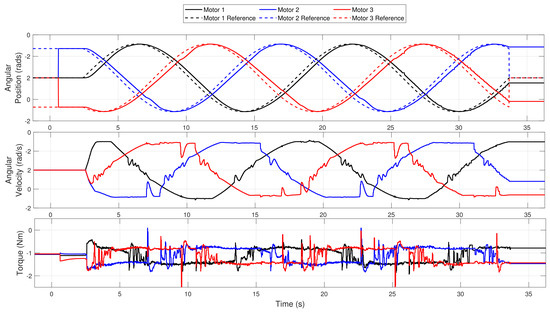
Figure 7. Motor positions, velocities, and torques for the considered motion experiment.

The experiment environment structure is illustrated in Figure 8. The control environment consists of two independent structures. The robot control structure operates via the Robot Operating System (ROS) Kinetic version, which runs on the Ubuntu OS. The ROS environment integrates tension sensors, Dynamixel motors, and control code. Additionally, we measured the robot trajectory using the Optitrack motion capture system in a Windows OS environment. Reflective markers were embedded on the tensegrity robot nodes to obtain the robot trajectory, as shown in Figure 4.

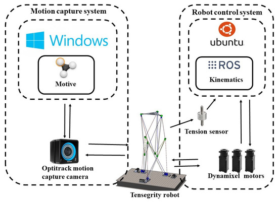
Figure 8. Tensegrity robot control environment.

Table 3 illustrates the average error between simulation and experiment. It can be seen that the error of the base nodes is significantly higher than that of the middle and upper plate nodes. This discrepancy is due to differences in the initial posture calibration of the base nodes, as shown in Table 1. The base nodes remain stationary during motion, resulting in no change in error rate. Conversely, the mid and upper nodes move along their trajectory, leading to a lower error rate than the initial posture.

Figure 9 shows the corresponding configurations of the simulator and experimental setup for different time instants during the motion generated by the motor profiles displayed in Figure 7; the full robot motion can be seen in the video provided as Supplementary Materials. As demonstrated in Figure 10, circular motions of the nodes correspond to the sinusoidal position profile of the motors; these circles have an increasing radius as the distance with the robot base increases.

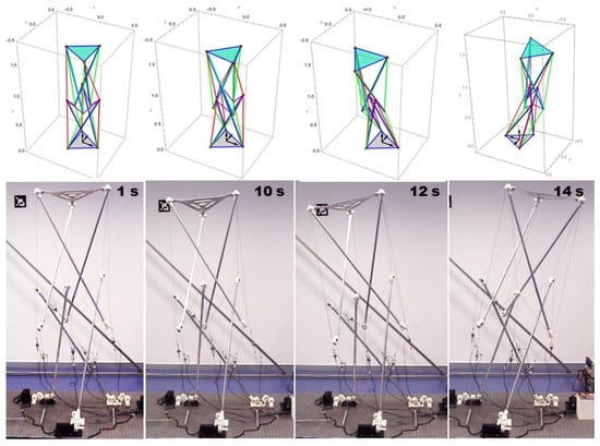
Figure 9. Comparison between configurations at different time instants of the considered experiment for simulator and actual tensegrity robot.

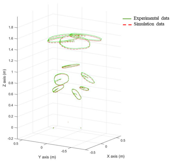
Figure 10. Tensegrity robot node trajectories provided from the Optitrack motion capture cameras.

To demonstrate the accuracy of our model, Figure 11 displays the overlay graph of the simulated trajectories in the considered experiment for node $n_{21}$. Based on the obtained result, this figure shows the validity of the proposed kinematic/kinetic formulation.

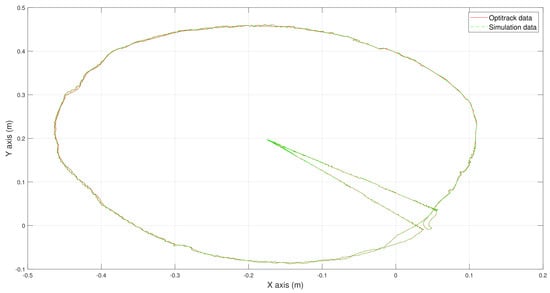
Figure 11. Comparison graph of experimental data (in blue) with simulation data (in green) for the time evolution of the x and y coordinates of node $n_{21}$.

5. Conclusions

The paper has presented a simplified combined formulation of kinematics and kinetics for prismatic tensegrity robots using a minimal set of coordinates. The definition of the proposed modeling framework is explained in detail for a laboratory prototype of a tensegrity robot. The provided experimental results show that the proposed modeling framework can provide an acceptable level of modeling accuracy, and thus be possibly employed in different applications. In this research paper, we presented a new formulation combined with kinematic and kinetic constraints and validated the proposed mathematical formulation by the simulation results. Moreover, the nodes’ position obtained in the simulation was compared with real tensegrity robot nodes’ position measured by MCS. The obtained results were consistently close, which was demonstrated in Table 2.

References

- Masic, M.; Skelton, R.E.; Gill, P.E. Optimization of tensegrity structures. Int. J. Solids Struct. 2006, 43, 4687–4703. [Google Scholar] [CrossRef]
- Zhang, Q.; Zhang, D.; Dobah, Y.; Scarpa, F.; Fraternali, F.; Skelton, R.E. Tensegrity cell mechanical metamaterial with metal rubber. Appl. Phys. Lett. 2018, 113, 031906. [Google Scholar] [CrossRef]
- Zhang, J.; Ohsaki, M. Stability conditions for tensegrity structures. Int. J. Solids Struct. 2007, 44, 3875–3886. [Google Scholar] [CrossRef]
- Sabelhaus, A.P.; Bruce, J.; Caluwaerts, K.; Manovi, P.; Firoozi, R.F.; Dobi, S.; Agogino, A.M.; SunSpiral, V. System design and locomotion of SUPERball, an untethered tensegrity robot. In Proceedings of the IEEE International Conference on Robotics and Automation (ICRA), Seattle, WA, USA, 26–30 May 2015; pp. 2867–2873. [Google Scholar]
- Calladine, C.R. Buckminster Fuller’s “tensegrity” structures and Clerk Maxwell’s rules for the construction of stiff frames. Int. J. Solids Struct. 1978, 14, 161–172. [Google Scholar] [CrossRef]
- Tibert, A.; Pellegrino, S. Review of form-finding methods for tensegrity structures. Int. J. Space Struct. 2003, 18, 209–223. [Google Scholar] [CrossRef]
- Tran, H.C.; Lee, J. Advanced form-finding of tensegrity structures. Comput. Struct. 2010, 88, 237–246. [Google Scholar] [CrossRef]
- Tran, H.; Lee, J. Form-finding of tensegrity structures with multiple states of self-stress. Acta Mech. 2011, 222, 131–147. [Google Scholar] [CrossRef]
- Montuori, R.; Skelton, R.E. Globally stable tensegrity compressive structures for arbitrary complexity. Compos. Struct. 2017, 179, 682–694. [Google Scholar] [CrossRef]
- Skelton, R.E.; Montuori, R.; Pecoraro, V. Globally stable minimal mass compressive tensegrity structures. Compos. Struct. 2016, 141, 346–354. [Google Scholar] [CrossRef]
- Lacagnina, M.; Russo, S.; Sinatra, R. A novel parallel manipulator architecture for manufacturing applications. Multibody Syst. Dyn. 2003, 10, 219–238. [Google Scholar] [CrossRef]
- Assal, S.F. Self-organizing approach for learning the forward kinematic multiple solutions of parallel manipulators. Robotica 2012, 30, 951–961. [Google Scholar] [CrossRef]
- Jeong, J.W.; Kim, S.H.; Kwak, Y.K.; Smith, C.C. Development of a parallel wire mechanism for measuring position and orientation of a robot end-effector. Mechatronics 1998, 8, 845–861. [Google Scholar] [CrossRef]
- Etemadi-zanganeh, K.; Angeles, J. Real-time direct kinematics of general six-degree-of-freedom parallel manipulators with minimum-sensor data. J. Robot. Syst. 1995, 12, 833–844. [Google Scholar] [CrossRef]
- Zheng, C.; Jiao, L. Forward kinematics of a general Stewart parallel manipulator using the genetic algorithm. J. Xidian Univ. (Nat. Sci.) 2003, 30, 165–168. [Google Scholar]
- Liu, S.; Li, Q.; Wang, P.; Guo, F. Kinematic and static analysis of a novel tensegrity robot. Mech. Mach. Theory 2020, 149, 103788. [Google Scholar] [CrossRef]
- Arsenault, M.; Gosselin, C.M. Kinematic and static analysis of a 3-PUPS spatial tensegrity mechanism. Mech. Mach. Theory 2009, 44, 162–179. [Google Scholar] [CrossRef]
- Murakami, H. Static and dynamic analyses of tensegrity structures. Part 1. Nonlinear equations of motion. Int. J. Solids Struct. 2001, 38, 3599–3613. [Google Scholar] [CrossRef]
- Zhang, L.; Maurin, B.; Motro, R. Form-finding of nonregular tensegrity systems. J. Struct. Eng. 2006, 132, 1435–1440. [Google Scholar] [CrossRef]
- Yamamoto, M.; Gan, B.; Fujita, K.; Kurokawa, J. A Genetic Algorithm Based Form-Finding for Tensegrity Structure. Procedia Eng. 2011, 14, 2949–2956. [Google Scholar] [CrossRef]
- Koohestani, K. Form-finding of tensegrity structures via genetic algorithm. Int. J. Solids Struct. 2012, 49, 739–747. [Google Scholar] [CrossRef]
- Pagitz, M.; Mirats Tur, J. Finite element based form-finding algorithm for tensegrity structures. Int. J. Solids Struct. 2009, 46, 3235–3240. [Google Scholar] [CrossRef]
- Estrada, G.G.; Bungartz, H.J.; Mohrdieck, C. Numerical form-finding of tensegrity structures. Int. J. Solids Struct. 2006, 43, 6855–6868. [Google Scholar] [CrossRef]
- Juan, S.H.; Mirats Tur, J.M. Tensegrity frameworks: Static analysis review. Mech. Mach. Theory 2008, 43, 859–881. [Google Scholar] [CrossRef]
- Sultan, C.; Corless, M.; Skelton, R.E. Linear dynamics of tensegrity structures. Eng. Struct. 2002, 24, 671–685. [Google Scholar] [CrossRef]
- Faroughi, S.; Khodaparast, H.H.; Friswell, M.I. Non-linear dynamic analysis of tensegrity structures using a co-rotational method. Int. J. Non-Linear Mech. 2015, 69, 55–65. [Google Scholar] [CrossRef]
- Skelton, R.E.; De Oliveira, M.C. Tensegrity Systems; Springer: Berlin/Heidelberg, Germany, 2009. [Google Scholar]
- Nagase, K.; Skelton, R. Network and vector forms of tensegrity system dynamics. Mech. Res. Commun. 2014, 59, 14–25. [Google Scholar] [CrossRef]
- Cheong, J.; Skelton, R.E. Nonminimal dynamics of general class k tensegrity systems. Int. J. Struct. Stab. Dyn. 2015, 15, 1450042. [Google Scholar] [CrossRef]
- Fadeyev, D.; Zhakatayev, A.; Kuzdeuov, A.; Varol, H.A. Generalized dynamics of stacked tensegrity manipulators. IEEE Access 2019, 7, 63472–63484. [Google Scholar] [CrossRef]
- Goyal, R.; Skelton, R.E. Tensegrity system dynamics with rigid bars and massive strings. Multibody Syst. Dyn. 2019, 46, 203–228. [Google Scholar] [CrossRef]
- Goyal, R.; Chen, M.; Majji, M.; Skelton, R.E. MOTES: Modeling of tensegrity structures. J. Open Source Softw. 2019, 4, 1613. [Google Scholar] [CrossRef]
- Lillo, P.D.; Chiaverini, S.; Antonelli, G. Handling robot constraints within a Set-Based Multi-Task Priority Inverse Kinematics Framework. In Proceedings of the 2019 International Conference on Robotics and Automation (ICRA), Montreal, QC, Canada, 20–24 May 2019; pp. 7477–7483. [Google Scholar] [CrossRef]
- Yun, A.; Ha, J. A geometric tracking of rank-1 manipulability for singularity-robust collision avoidance. Intell. Serv. Robot. 2021, 14, 271–284. [Google Scholar] [CrossRef]
- Mohamed, N.A.; Azar, A.T.; Abbas, N.E.; Ezzeldin, M.A.; Ammar, H.H. Experimental kinematic modeling of 6-dof serial manipulator using hybrid deep learning. In Proceedings of the International Conference on Artificial Intelligence and Computer Vision, Cairo, Egypt, 8–10 April 2020; pp. 283–295. [Google Scholar]
- Liu, Y.; Bi, Q.; Yue, X.; Wu, J.; Yang, B.; Li, Y. A review on tensegrity structures-based robots. Mech. Mach. Theory 2022, 168, 104571. [Google Scholar] [CrossRef]
- Shah, D.S.; Booth, J.W.; Baines, R.L.; Wang, K.; Vespignani, M.; Bekris, K.; Kramer-Bottiglio, R. Tensegrity Robotics. Soft Robot. 2022, 9, 639–656. [Google Scholar] [CrossRef]
- Mintchev, S.; Zappetti, D.; Willemin, J.; Floreano, D. A Soft Robot for Random Exploration of Terrestrial Environments. In Proceedings of the IEEE International Conference on Robotics and Automation (ICRA), Brisbane, Australia, 21–25 May 2018; pp. 7492–7497. [Google Scholar] [CrossRef]
- Hao, S.; Liu, R.; Lin, X.; Li, C.; Guo, H.; Ye, Z.; Wang, C. Configuration Design and Gait Planning of a Six-Bar Tensegrity Robot. Appl. Sci. 2022, 12, 11845. [Google Scholar] [CrossRef]
- Li, W.Y.; Nabae, H.; Endo, G.; Suzumori, K. New soft robot hand configuration with combined biotensegrity and thin artificial muscle. IEEE Robot. Autom. Lett. 2020, 5, 4345–4351. [Google Scholar] [CrossRef]
- Kawahara, K.; Shin, D.; Ogai, Y. Design of a Movable Tensegrity Arm with Springs Modeling an Upper and Lower Arm. Actuators 2023, 12, 18. [Google Scholar] [CrossRef]
- Wang, T.; Post, M.A. A Symmetric Three Degree of Freedom Tensegrity Mechanism with Dual Operation Modes for Robot Actuation. Biomimetics 2021, 6, 30. [Google Scholar] [CrossRef]
- Chen, B.; Jiang, H. Swimming performance of a tensegrity robotic fish. Soft Robot. 2019, 6, 520–531. [Google Scholar] [CrossRef]
- Zhang, P.; Kawaguchi, K.; Feng, J. Prismatic tensegrity structures with additional cables: Integral symmetric states of self-stress and cable-controlled reconfiguration procedure. Int. J. Solids Struct. 2014, 51, 4294–4306. [Google Scholar] [CrossRef]
- Zhang, J.; Guest, S.; Ohsaki, M. Symmetric prismatic tensegrity structures: Part I. Configuration and stability. Int. J. Solids Struct. 2009, 46, 1–14. [Google Scholar] [CrossRef]
- Li, Y.; Feng, X.Q.; Cao, Y.P.; Gao, H. A Monte Carlo form-finding method for large scale regular and irregular tensegrity structures. Int. J. Solids Struct. 2010, 47, 1888–1898. [Google Scholar] [CrossRef]
- Brahmia, A.; Kelaiaia, R.; Chemori, A.; Company, O. On Robust Mechanical Design of a PAR2 Delta-Like Parallel Kinematic Manipulator. J. Mech. Robot. 2021, 14, 011001. [Google Scholar] [CrossRef]
- Kelaiaia, R.; Zaatri, A.; Company, O. Multiobjective Optimization of 6-dof UPS Parallel Manipulators. Adv. Robot. 2012, 26, 1885–1913. [Google Scholar] [CrossRef]
- Yeshmukhametov, A.; Koganezawa, K.; Yamamoto, Y. A novel discrete wire-driven continuum robot arm with passive sliding disc: Design, kinematics and passive tension control. Robotics 2019, 8, 51. [Google Scholar] [CrossRef]
- Yeshmukhametov, A.N.; Koganezawa, K.; Buribayev, Z.; Amirgaliyev, Y.; Yamamoto, Y. Study on multi-section continuum robot wire-tension feedback control and load manipulability. Ind. Robot Int. J. Robot. Res. Appl. 2020, 47, 837–845. [Google Scholar] [CrossRef]
- Gill, P.E.; Jay, L.O.; Leonard, M.W.; Petzold, L.R.; Sharma, V. An SQP method for the optimal control of large-scale dynamical systems. J. Comput. Appl. Math. 2000, 120, 197–213. [Google Scholar] [CrossRef]
- Wright, S.J. Interior point methods for optimal control of discrete time systems. J. Optim. Theory Appl. 1993, 77, 161–187. [Google Scholar] [CrossRef]
- Mattingley, J.; Boyd, S. CVXGEN: A code generator for embedded convex optimization. Optim. Eng. 2012, 13, 1–27. [Google Scholar] [CrossRef]
- Verschueren, R.; Frison, G.; Kouzoupis, D.; Frey, J.; Duijkeren, N.v.; Zanelli, A.; Novoselnik, B.; Albin, T.; Quirynen, R.; Diehl, M. acados—A modular open-source framework for fast embedded optimal control. Math. Program. Comput. 2022, 14, 147–183. [Google Scholar] [CrossRef]
Disclaimer/Publisher’s Note: The statements, opinions and data contained in all publications are solely those of the individual author(s) and contributor(s) and not of MDPI and/or the editor(s). MDPI and/or the editor(s) disclaim responsibility for any injury to people or property resulting from any ideas, methods, instructions or products referred to in the content. |
© 2023 by the authors. Licensee MDPI, Basel, Switzerland. This article is an open access article distributed under the terms and conditions of the Creative Commons Attribution (CC BY) license (https://creativecommons.org/licenses/by/4.0/).